25  Epipolar Geometry

25.1 Two-View Geometry

A single camera sees directions, not distances: every image point corresponds to a ray in 3D space, and without additional information you cannot tell whether a scene point is near or far along that ray. Two cameras fix this: the same 3D point \(\mathbf{X} \in \mathbb{R}^3\) projects to image point \(\mathbf{x}_1\) in camera 1 and \(\mathbf{x}_2\) in camera 2, and the intersection of the two back-projected rays gives the depth.

This section sets up the geometry precisely and introduces three objects — the epipole, the epipolar plane, and epipolar lines — that constrain where a point seen in one image must appear in the other.

---

25.1.1 Camera Model Recap

Recall from Chapter 10 that a pinhole camera with intrinsic matrix \(K \in \mathbb{R}^{3 \times 3}\), rotation \(R\), and translation \(\mathbf{t}\) maps a world point \(\mathbf{X}_h = [\mathbf{X}^T, 1]^T\) to a pixel via

\[ \lambda \mathbf{x} = P\, \mathbf{X}_h, \qquad P = K\,[R \mid \mathbf{t}] \in \mathbb{R}^{3 \times 4}. \tag{25.1} \]

Place camera 1 at the world origin: \(P_1 = K\,[\,I \mid \mathbf{0}\,]\). Camera 2 has center \(\mathbf{C}_2\) and orientation \(R_2\) in world coordinates, so \(\mathbf{t}_2 = -R_2 \mathbf{C}_2\) and \(P_2 = K\,[R_2 \mid \mathbf{t}_2]\).

The epipole \(\mathbf{e}_1\) is the projection of camera 2’s center into camera 1’s image, and \(\mathbf{e}_2\) is the projection of camera 1’s center (the world origin) into camera 2:

\[ \lambda_1\, \mathbf{e}_1 = P_1 \begin{bmatrix}\mathbf{C}_2 \\ 1\end{bmatrix}, \qquad \lambda_2\, \mathbf{e}_2 = P_2 \begin{bmatrix}\mathbf{0} \\ 1\end{bmatrix}. \tag{25.2} \]

The epipolar plane through \(\mathbf{X}\), camera 1’s center \(\mathbf{O}_1 = \mathbf{0}\), and camera 2’s center \(\mathbf{C}_2\) is a flat triangle in 3D. Its intersections with the two image planes are the epipolar lines \(\ell_1\) and \(\ell_2\).

---

25.1.2 The Epipolar Constraint

The epipolar constraint says that corresponding image points must each lie on the other camera’s epipolar line. If \(\mathbf{x}_1\) is a point in image 1, its epipolar line in image 2 is

\[ \ell_2 = F\,\mathbf{x}_1, \tag{25.3} \]

where \(F\) is the fundamental matrix (§25.3). The constraint \(\mathbf{x}_2^T F\,\mathbf{x}_1 = 0\) encodes exactly that \(\mathbf{x}_2\) lies on \(\ell_2\).

This is powerful: instead of searching the entire image for a match to \(\mathbf{x}_1\), you need only search along a line — reducing the correspondence problem from 2D to 1D.

---

25.1.3 Visualization: Epipolar Lines

The code below sets up two cameras sharing the same intrinsic matrix, places five 3D scene points, and draws the epipolar lines each image point induces in the other image.

import numpy as np
import matplotlib.pyplot as plt
import matplotlib.patches as mpatches

rng = np.random.default_rng(7)

# ---- camera setup ----
K = np.array([[500., 0., 320.],
              [0., 500., 240.],
              [0., 0.,   1.]])    # shape (3, 3)

# Camera 1 at world origin
R1 = np.eye(3)                   # shape (3, 3)
t1 = np.zeros(3)                 # shape (3,)
P1 = K @ np.hstack([R1, t1.reshape(3, 1)])   # shape (3, 4)

# Camera 2 displaced along x, slight y offset
C2 = np.array([0.4, -0.1, 0.0])  # world position of camera 2 center
R2 = np.eye(3)                    # shape (3, 3)
t2 = -R2 @ C2                    # shape (3,)
P2 = K @ np.hstack([R2, t2.reshape(3, 1)])   # shape (3, 4)

W, H = 640., 480.

# ---- helper: project homogeneous point to pixel ----
def project(P, X):
    lam_x = P @ np.append(X, 1.)    # shape (3,)
    return lam_x[:2] / lam_x[2]     # shape (2,)

# ---- helper: clip line ax+by+c=0 to image ----
def clip_line(l, W, H):
    a, b, c = float(l[0]), float(l[1]), float(l[2])
    cands = []
    if abs(b) > 1e-10:
        for u in [0., W]:
            v = -(a * u + c) / b
            if 0. <= v <= H:
                cands.append([u, v])
    if abs(a) > 1e-10:
        for v in [0., H]:
            u = -(b * v + c) / a
            if 0. <= u <= W:
                cands.append([u, v])
    unique = []
    for p in cands:
        if not any(np.allclose(p, q) for q in unique):
            unique.append(p)
    return np.array(unique[:2]) if len(unique) >= 2 else None

# ---- 5 scene points in front of both cameras ----
X_world = np.array([
    [-0.3,  0.2, 3.0],
    [ 0.0, -0.1, 2.5],
    [ 0.2,  0.3, 3.5],
    [ 0.4,  0.0, 2.8],
    [-0.1, -0.3, 3.2],
])  # shape (5, 3)

# project to both images
x1s = np.array([project(P1, X) for X in X_world])  # shape (5, 2)
x2s = np.array([project(P2, X) for X in X_world])  # shape (5, 2)

# ---- epipoles ----
lam_e1 = P1 @ np.append(C2, 1.)    # shape (3,)
e1 = lam_e1[:2] / lam_e1[2]        # shape (2,)

lam_e2 = P2 @ np.array([0., 0., 0., 1.])    # shape (3,)
e2 = lam_e2[:2] / lam_e2[2]                  # shape (2,)

# ---- skew-symmetric matrix ----
def skew(v):
    return np.array([[ 0.,    -v[2],  v[1]],
                     [ v[2],   0.,   -v[0]],
                     [-v[1],  v[0],   0.  ]])  # shape (3, 3)

# baseline translation in camera-1 frame
t_12 = t2 - t1    # shape (3,)
E = skew(t_12) @ R2   # shape (3, 3)  (essential matrix, same R since R1=I)
F = np.linalg.inv(K).T @ E @ np.linalg.inv(K)   # shape (3, 3)

# ---- draw ----
fig, axes = plt.subplots(1, 2, figsize=(12, 5))
colors = ['#4a90d9', '#2ecc71', 'goldenrod', 'orchid', 'coral']

for ax, cam, x_self, x_other, F_dir, epole, title in [
    (axes[0], 'Image 1', x1s, x2s, F.T,  e1, 'Camera 1 (points + epipole)'),
    (axes[1], 'Image 2', x2s, x1s, F,    e2, 'Camera 2 (epipolar lines + epipole)'),
]:
    ax.set_xlim(0, W); ax.set_ylim(H, 0)
    ax.set_aspect('equal')
    ax.set_facecolor('#f8f8f8')
    ax.set_title(title, fontsize=10)
    ax.set_xlabel('u (px)'); ax.set_ylabel('v (px)')

    for i, (xi, xo) in enumerate(zip(x_self, x_other)):
        c = colors[i % len(colors)]
        ax.scatter(*xi, color=c, s=50, zorder=5)
        # draw epipolar line induced by the OTHER image's point
        xo_h = np.append(xo, 1.)    # shape (3,)
        l = F_dir @ xo_h            # shape (3,)
        seg = clip_line(l, W, H)
        if seg is not None:
            ax.plot(seg[:, 0], seg[:, 1], color=c, lw=1.2, alpha=0.7)

    ax.scatter(*epole, marker='*', s=160, color='tomato', zorder=6, label=f'epipole')
    ax.legend(fontsize=8)

plt.tight_layout()
plt.show()

print(f"Epipole e1 (camera 2 center in image 1): ({e1[0]:.1f}, {e1[1]:.1f})")
print(f"Epipole e2 (camera 1 center in image 2): ({e2[0]:.1f}, {e2[1]:.1f})")

C:\Users\james.choi\AppData\Local\Temp\ipykernel_11136\2086319340.py:65: RuntimeWarning: divide by zero encountered in divide
  e1 = lam_e1[:2] / lam_e1[2]        # shape (2,)
C:\Users\james.choi\AppData\Local\Temp\ipykernel_11136\2086319340.py:68: RuntimeWarning: divide by zero encountered in divide
  e2 = lam_e2[:2] / lam_e2[2]                  # shape (2,)

Figure 25.1: Epipolar geometry for two cameras. Left: image 1 shows scene points (blue dots) and the epipole e1 (red star). Right: image 2 shows the corresponding epipolar lines – each blue point in image 1 generates one red line in image 2 that constrains where the match must lie.

Epipole e1 (camera 2 center in image 1): (inf, -inf)
Epipole e2 (camera 1 center in image 2): (-inf, inf)

Each color corresponds to one 3D point. The blue dot at position \(\mathbf{x}_1\) in image 1 constrains its match in image 2 to lie on the blue line — a 1D search instead of a 2D search. All epipolar lines in one image pass through that image’s epipole.

---

25.1.4 Summary of Relationships

Object	Definition	Dimension
Epipole \(\mathbf{e}_1\)	Projection of \(\mathbf{C}_2\) into image 1	1 point
Epipole \(\mathbf{e}_2\)	Projection of \(\mathbf{O}_1\) into image 2	1 point
Epipolar plane	Plane through \(\mathbf{X}\), \(\mathbf{O}_1\), \(\mathbf{C}_2\)	varies per point
Epipolar line \(\ell_2\)	Intersection of epipolar plane with image 2	1 line per point
Fundamental matrix \(F\)	Maps \(\mathbf{x}_1 \mapsto \ell_2 = F\mathbf{x}_1\)	\(3 \times 3\), rank 2

The fundamental matrix \(F\) encodes the complete epipolar geometry of a camera pair. The next two sections derive it from first principles.

---

25.1.5 Exercises

1. Show that every epipolar line in image 2 passes through \(\mathbf{e}_2\). (Hint: \(F\mathbf{e}_1 = \mathbf{0}\) and \(F^T \mathbf{e}_2 = \mathbf{0}\).)
2. If both cameras have the same center (\(\mathbf{C}_1 = \mathbf{C}_2\)), where do the epipoles lie and what happens to the epipolar lines?
3. In the visualization above, move camera 2 to \(\mathbf{C}_2 = [2, 0, 0]\) (far to the right). Predict qualitatively where the epipole \(\mathbf{e}_1\) will appear, then verify by rerunning the code.

25.2 The Essential Matrix \(E = [\mathbf{t}]_\times R\)

When the intrinsic parameters \(K\) of both cameras are known, it is natural to work in normalized image coordinates: divide pixel coordinates by \(K\) and treat each image point as a unit-depth ray direction. The essential matrix \(E\) captures the relative pose \((R, \mathbf{t})\) between two calibrated cameras and enforces the epipolar constraint in normalized coordinates.

---

25.2.1 Setup: Normalized Coordinates

Let \(\mathbf{y} = K^{-1}\mathbf{x} \in \mathbb{R}^3\) be the normalized (homogeneous) image point for pixel \(\mathbf{x}\). The back-projected ray in camera 1’s frame is \(\lambda_1 \mathbf{y}_1\) for some unknown depth \(\lambda_1 > 0\).

Camera 2’s frame is related to camera 1’s by rotation \(R\) and translation \(\mathbf{t}\) (the pose of camera 2 expressed in camera 1’s coordinates). A world point seen at depth \(\lambda_1\) in camera 1 satisfies

\[ \lambda_2\, \mathbf{y}_2 = R\,(\lambda_1\, \mathbf{y}_1) + \mathbf{t}, \tag{25.4} \]

with \(\lambda_2 > 0\) the depth in camera 2.

---

25.2.2 Deriving the Coplanarity Constraint

Pre-multiply both sides of (25.4) by \([\mathbf{t}]_\times\) (the skew-symmetric matrix encoding the cross product with \(\mathbf{t}\), introduced in Chapter 8):

\[ \lambda_2\, [\mathbf{t}]_\times \mathbf{y}_2 = [\mathbf{t}]_\times R\,\lambda_1\, \mathbf{y}_1 + \underbrace{[\mathbf{t}]_\times \mathbf{t}}_{=\,\mathbf{0}}. \]

Now take the dot product with \(\mathbf{y}_2\):

\[ \lambda_2\, \mathbf{y}_2^T\, [\mathbf{t}]_\times \mathbf{y}_2 = \lambda_1\, \mathbf{y}_2^T\, [\mathbf{t}]_\times R\, \mathbf{y}_1. \]

The left side is \(\mathbf{y}_2 \cdot (\mathbf{t} \times \mathbf{y}_2) = 0\) (a vector crossed with itself yields zero). Dividing by \(\lambda_1 \lambda_2 > 0\) gives the coplanarity constraint:

\[ \boxed{\mathbf{y}_2^T\, E\, \mathbf{y}_1 = 0, \qquad E = [\mathbf{t}]_\times R.} \tag{25.5} \]

Geometrically, \(\mathbf{y}_1\), \(\mathbf{y}_2\), and \(\mathbf{t}\) are coplanar: all three lie in the epipolar plane. The essential matrix encodes exactly this triple-product condition.

---

25.2.3 Degrees of Freedom and Algebraic Properties

The relative pose \((R, \mathbf{t})\) has \(3 + 3 = 6\) degrees of freedom, but the overall scale of \(\mathbf{t}\) is unobservable from image correspondences alone (you can only recover the direction of translation, not its magnitude). Therefore \(E\) has \(6 - 1 = 5\) degrees of freedom.

Note

Properties of \(E\). - \(\operatorname{rank}(E) = 2\) (det \(E = 0\) because \([\mathbf{t}]_\times\) has rank 2). - The two nonzero singular values of \(E\) are equal: if \(E = U\Sigma V^T\) then \(\Sigma = \text{diag}(\sigma, \sigma, 0)\). - \(E^T \mathbf{e}_2 = \mathbf{0}\) and \(E\, \mathbf{e}_1 = \mathbf{0}\), so the epipoles are the right and left null vectors of \(E\).

The equal-singular-value condition is the algebraic signature that distinguishes a valid essential matrix from an arbitrary rank-2 matrix.

---

25.2.4 Code: Verify Essential Matrix Properties

import numpy as np
import matplotlib.pyplot as plt
from scipy.spatial.transform import Rotation

rng = np.random.default_rng(42)

# ---- ground-truth relative pose ----
rotvec = rng.normal(0., 0.3, 3)                     # shape (3,)
R_true = Rotation.from_rotvec(rotvec).as_matrix()   # shape (3, 3)
t_true = np.array([0.4, -0.1, 0.2])                 # shape (3,)   (unit-scale)
t_true = t_true / np.linalg.norm(t_true)            # shape (3,)

def skew(v):
    return np.array([[ 0.,    -v[2],  v[1]],
                     [ v[2],   0.,   -v[0]],
                     [-v[1],  v[0],   0.  ]])    # shape (3, 3)

E = skew(t_true) @ R_true    # shape (3, 3)

# ---- singular values ----
s = np.linalg.svd(E, compute_uv=False)    # shape (3,)  -- returns array, not tuple

# ---- 200 random scene points, project to both cameras ----
n = 200
X_world = rng.uniform(-0.5, 0.5, (n, 3)) + np.array([0., 0., 3.])   # shape (200, 3)

# camera 1 rays (normalized): just divide by z
y1s = X_world / X_world[:, 2:3]    # shape (200, 3)

# camera 2 rays: apply R, t then normalize
X_cam2 = (R_true @ X_world.T).T + t_true    # shape (200, 3)
y2s = X_cam2 / X_cam2[:, 2:3]               # shape (200, 3)

# algebraic residuals
residuals = np.array([y2s[i] @ E @ y1s[i] for i in range(n)])    # shape (200,)

# ---- plot ----
fig, axes = plt.subplots(1, 2, figsize=(11, 4))

ax = axes[0]
ax.bar(['sigma_1', 'sigma_2', 'sigma_3'], s, color=['#4a90d9', '#4a90d9', 'tomato'])
ax.set_title('Singular values of E')
ax.set_ylabel('Value')
ax.grid(alpha=0.2, axis='y')
ax.text(0, s[0] + 0.01, f'{s[0]:.4f}', ha='center', fontsize=9)
ax.text(1, s[1] + 0.01, f'{s[1]:.4f}', ha='center', fontsize=9)
ax.text(2, s[2] + 0.01, f'{s[2]:.2e}', ha='center', fontsize=9)

ax = axes[1]
ax.semilogy(np.abs(residuals), color='#4a90d9', lw=0.8, alpha=0.7)
ax.set_xlabel('Correspondence index')
ax.set_ylabel(r'$|y_2^T E y_1|$ (log scale)')
ax.set_title('Coplanarity residuals')
ax.grid(alpha=0.2)

plt.tight_layout()
plt.show()

print(f"sigma_1 = {s[0]:.6f},  sigma_2 = {s[1]:.6f},  sigma_3 = {s[2]:.2e}")
print(f"Equal singular values: {np.isclose(s[0], s[1])}")
print(f"Max coplanarity residual: {np.abs(residuals).max():.2e}")

Figure 25.2: Singular values of E and the algebraic residual |y2^T E y1| for 200 random calibrated correspondences. Left: the two nonzero singular values are exactly equal by construction. Right: residuals are at machine-precision zero, confirming the coplanarity constraint.

sigma_1 = 1.000000,  sigma_2 = 1.000000,  sigma_3 = 3.05e-17
Equal singular values: True
Max coplanarity residual: 8.33e-17

Both nonzero singular values are equal to machine precision, confirming that \(E\) satisfies the essential-matrix constraints by construction.

---

25.2.5 Geometric Interpretation

The constraint \(\mathbf{y}_2^T E\,\mathbf{y}_1 = 0\) is a scalar equation in two homogeneous 2D points. It says that \(\mathbf{y}_1\), \(\mathbf{y}_2\), and \(\mathbf{t}\) are coplanar — they span a 2D plane in 3D space, the epipolar plane of §25.1.

\(E\,\mathbf{y}_1\) is the normal to the epipolar plane expressed in camera 2’s coordinates: it defines the epipolar line in camera 2’s normalized image. Similarly, \(E^T \mathbf{y}_2\) is the epipolar line in camera 1’s normalized image.

---

25.2.6 Exercises

1. Show that \(\det([\mathbf{t}]_\times) = 0\) for any nonzero \(\mathbf{t}\), and hence \(\operatorname{rank}(E) \leq 2\). Then argue that \(\operatorname{rank}(E) = 2\) (not 1 or 0) for generic \(R\) and \(\mathbf{t}\).
2. Verify algebraically that the two nonzero singular values of \(E = [\mathbf{t}]_\times R\) are both equal to \(\|\mathbf{t}\|\). (Hint: compute \(E^T E = R^T [\mathbf{t}]_\times^T [\mathbf{t}]_\times R\) and use \([\mathbf{t}]_\times^T [\mathbf{t}]_\times = \|\mathbf{t}\|^2 I - \mathbf{t}\mathbf{t}^T\).)
3. If you scale the translation by \(\alpha > 0\) to get \(E' = [\alpha\mathbf{t}]_\times R\), show that the coplanarity constraint \(\mathbf{y}_2^T E' \mathbf{y}_1 = 0\) is unchanged. This confirms that only the direction of \(\mathbf{t}\) is recoverable from image correspondences.

25.3 The Fundamental Matrix \(F = K'^{-T} E K^{-1}\)

The essential matrix works in normalized coordinates and requires knowing \(K\). In many practical settings the intrinsic parameters are unavailable or approximate. The fundamental matrix \(F\) generalizes the epipolar constraint to raw pixel coordinates, absorbing \(K\) into the matrix itself.

---

25.3.1 From Pixels to Normalized Coordinates

A pixel \(\mathbf{x} = [u, v, 1]^T\) maps to a normalized ray via

\[ \mathbf{y} = K^{-1}\mathbf{x}. \tag{25.6} \]

Substituting into the essential matrix constraint \(\mathbf{y}_2^T E\,\mathbf{y}_1 = 0\):

\[ (K'^{-1}\mathbf{x}_2)^T\, E\,(K^{-1}\mathbf{x}_1) = 0, \]

where \(K'\) is the intrinsic matrix of camera 2 (possibly different from camera 1’s \(K\)). Rearranging:

\[ \mathbf{x}_2^T \underbrace{K'^{-T} E\, K^{-1}}_{F} \mathbf{x}_1 = 0. \tag{25.7} \]

The fundamental matrix is therefore

\[ \boxed{F = K'^{-T} E\, K^{-1} = K'^{-T}\, [\mathbf{t}]_\times R\, K^{-1}.} \tag{25.8} \]

---

25.3.2 Degrees of Freedom

\(F\) is a \(3 \times 3\) homogeneous matrix (\(-1\) DOF for scale), with the additional constraint \(\det(F) = 0\) (\(-1\) DOF for rank-2). It has \(9 - 1 - 1 = 7\) degrees of freedom. Compared to \(E\)’s 5 DOF, the extra 2 encode the unknown intrinsics.

Note

Properties of \(F\). - \(\operatorname{rank}(F) = 2\), same as \(E\). - \(F^T \mathbf{e}_2 = \mathbf{0}\) and \(F\,\mathbf{e}_1 = \mathbf{0}\): the epipoles are the null vectors of \(F\) and \(F^T\). - \(F\) is only defined up to scale. - Unlike \(E\), the two nonzero singular values of \(F\) are generally unequal.

---

25.3.3 Epipolar Lines in Pixel Coordinates

Given a pixel \(\mathbf{x}_1\) in image 1, its epipolar line in image 2 is

\[ \boldsymbol{\ell}_2 = F\,\mathbf{x}_1 \in \mathbb{R}^3, \tag{25.9} \]

where \(\boldsymbol{\ell}_2 = [a, b, c]^T\) encodes the line \(au + bv + c = 0\) in image 2. The symmetric relation holds: \(\boldsymbol{\ell}_1 = F^T\mathbf{x}_2\).

---

25.3.4 Code: F from Known K and Visualizing Epipolar Lines

The code below computes \(F\) analytically from known \(K\), \(R\), \(\mathbf{t}\) and verifies the constraint on synthetic correspondences.

import numpy as np
import matplotlib.pyplot as plt
from scipy.spatial.transform import Rotation

rng = np.random.default_rng(13)

# ---- camera setup ----
K = np.array([[600.,  0., 320.],
              [  0., 600., 240.],
              [  0.,   0.,   1.]])    # shape (3, 3)

# camera 2 has a different intrinsic (different focal length)
K2 = np.array([[580.,  0., 310.],
               [  0., 580., 235.],
               [  0.,   0.,   1.]])   # shape (3, 3)

def skew(v):
    return np.array([[ 0.,    -v[2],  v[1]],
                     [ v[2],   0.,   -v[0]],
                     [-v[1],  v[0],   0.  ]])    # shape (3, 3)

# relative pose: camera 2 relative to camera 1
R_rel = Rotation.from_euler('y', 8., degrees=True).as_matrix()   # shape (3, 3)
t_rel = np.array([0.5, 0.05, 0.0])                                # shape (3,)

E = skew(t_rel) @ R_rel          # shape (3, 3)
F = np.linalg.inv(K2).T @ E @ np.linalg.inv(K)    # shape (3, 3)
F = F / np.linalg.norm(F)        # normalize to unit Frobenius norm

# ---- scene points ----
n = 6
X_world = rng.uniform(-0.4, 0.4, (n, 3)) + np.array([0., 0., 3.0])  # shape (6, 3)

# project into both cameras
P1 = K  @ np.hstack([np.eye(3), np.zeros((3, 1))])    # shape (3, 4)
t2_world = t_rel.copy()                                 # shape (3,)
P2 = K2 @ np.hstack([R_rel, t2_world.reshape(3, 1)])  # shape (3, 4)

def project(P, X):
    lam_x = P @ np.append(X, 1.)
    return lam_x[:2] / lam_x[2]    # shape (2,)

x1s = np.array([project(P1, X) for X in X_world])    # shape (6, 2)
x2s = np.array([project(P2, X) for X in X_world])    # shape (6, 2)

# verify constraint
x1h = np.hstack([x1s, np.ones((n, 1))])   # shape (6, 3)
x2h = np.hstack([x2s, np.ones((n, 1))])   # shape (6, 3)
residuals = np.array([x2h[i] @ F @ x1h[i] for i in range(n)])    # shape (6,)

# ---- clip line ----
W, H = 640., 480.
def clip_line(l, W, H):
    a, b, c = float(l[0]), float(l[1]), float(l[2])
    cands = []
    if abs(b) > 1e-10:
        for u in [0., W]:
            v = -(a * u + c) / b
            if 0. <= v <= H:
                cands.append([u, v])
    if abs(a) > 1e-10:
        for v in [0., H]:
            u = -(b * v + c) / a
            if 0. <= u <= W:
                cands.append([u, v])
    unique = []
    for p in cands:
        if not any(np.allclose(p, q) for q in unique):
            unique.append(p)
    return np.array(unique[:2]) if len(unique) >= 2 else None

# ---- draw ----
colors = ['#4a90d9', '#2ecc71', 'goldenrod', 'orchid', 'coral', 'steelblue']
fig, axes = plt.subplots(1, 2, figsize=(12, 5))

axes[0].set_title('Image 1 -- points', fontsize=10)
axes[1].set_title('Image 2 -- epipolar lines (from F x1)', fontsize=10)

for ax in axes:
    ax.set_xlim(0, W); ax.set_ylim(H, 0)
    ax.set_aspect('equal')
    ax.set_facecolor('#f8f8f8')
    ax.set_xlabel('u (px)'); ax.set_ylabel('v (px)')

for i in range(n):
    c = colors[i % len(colors)]
    axes[0].scatter(x1s[i, 0], x1s[i, 1], color=c, s=55, zorder=5)
    axes[1].scatter(x2s[i, 0], x2s[i, 1], color=c, s=55, zorder=5)
    l2 = F @ np.append(x1s[i], 1.)    # shape (3,)
    seg = clip_line(l2, W, H)
    if seg is not None:
        axes[1].plot(seg[:, 0], seg[:, 1], color=c, lw=1.5, alpha=0.8)

# epipoles
Kt_inv_e1 = np.linalg.solve(K,  np.append(t2_world, 1.)[:3])  # approx for display
lam_e1 = P1 @ np.append(np.linalg.inv(R_rel) @ (-t2_world), 1.)
e1 = lam_e1[:2] / lam_e1[2]     # shape (2,)
lam_e2 = P2 @ np.array([0., 0., 0., 1.])
e2 = lam_e2[:2] / lam_e2[2]     # shape (2,)
axes[0].scatter(*e1, marker='*', s=160, color='tomato', zorder=6, label='e1')
axes[1].scatter(*e2, marker='*', s=160, color='tomato', zorder=6, label='e2')
axes[0].legend(fontsize=8); axes[1].legend(fontsize=8)

plt.tight_layout()
plt.show()

print(f"rank(F) via singular values: {np.linalg.matrix_rank(F)}")
print(f"Max constraint residual |x2^T F x1|: {np.abs(residuals).max():.2e}")

C:\Users\james.choi\AppData\Local\Temp\ipykernel_11136\2625025920.py:99: RuntimeWarning: divide by zero encountered in divide
  e2 = lam_e2[:2] / lam_e2[2]     # shape (2,)

Figure 25.3: Epipolar lines generated by the fundamental matrix. Six color-coded points in image 1 (left) each generate a corresponding epipolar line in image 2 (right). The match for each point must lie on its colored line.

rank(F) via singular values: 2
Max constraint residual |x2^T F x1|: 1.42e-14

The rank-2 property of \(F\) is confirmed, and all epipolar residuals are at machine precision.

---

25.3.5 Transferring Between E and F

When \(K\) is known, \(E\) and \(F\) carry the same information and are interchangeable:

\[ E = K'^T F K, \qquad F = K'^{-T} E K^{-1}. \tag{25.10} \]

In practice, \(F\) is estimated first (§25.4) and \(E\) is recovered by multiplying by \(K\) if the camera is calibrated.

---

25.3.6 Exercises

1. Show that \(F\) has rank 2 given that \(E\) has rank 2 and \(K\), \(K'\) are invertible.
2. Prove that the epipoles satisfy \(F\mathbf{e}_1 = \mathbf{0}\) and \(F^T \mathbf{e}_2 = \mathbf{0}\) by tracing through equations (25.8) and (25.2).
3. A point \(\mathbf{x}_1\) in image 1 satisfies \(\mathbf{x}_2^T F \mathbf{x}_1 = 0\) for all points \(\mathbf{x}_2\) on the epipolar line \(\ell_2\). What geometric condition does this express? Relate it to the triple-product argument used to derive \(E\).

25.4 Eight-Point Algorithm

Given a set of pixel correspondences \((\mathbf{x}_1^{(i)}, \mathbf{x}_2^{(i)})\) extracted by a feature detector (SIFT, ORB, etc.), the eight-point algorithm estimates the fundamental matrix \(F\) directly from the epipolar constraint, without requiring calibration.

---

25.4.1 Linear System: \(Af = 0\)

Expand the constraint \(\mathbf{x}_2^T F\,\mathbf{x}_1 = 0\) for correspondence \(i\). Writing \(\mathbf{x}_1 = [u_1, v_1, 1]^T\) and \(\mathbf{x}_2 = [u_2, v_2, 1]^T\), and vectorizing \(F\) row-by-row into \(\mathbf{f} \in \mathbb{R}^9\), gives a single linear equation in \(\mathbf{f}\):

\[ \mathbf{a}_i^T \mathbf{f} = 0, \qquad \mathbf{a}_i = \mathbf{x}_2 \otimes \mathbf{x}_1 = [u_2 u_1,\; u_2 v_1,\; u_2,\; v_2 u_1,\; v_2 v_1,\; v_2,\; u_1,\; v_1,\; 1]^T. \tag{25.11} \]

Stacking \(n \geq 8\) correspondences forms the \(n \times 9\) system

\[ A\mathbf{f} = \mathbf{0}, \qquad A \in \mathbb{R}^{n \times 9}. \tag{25.12} \]

Solve via SVD: the solution is the right singular vector corresponding to the smallest singular value of \(A\). Then reshape \(\mathbf{f}\) into a \(3 \times 3\) matrix \(F_{\text{raw}}\).

---

25.4.2 Rank-2 Enforcement

The SVD solution \(F_{\text{raw}}\) generally has rank 3. To enforce rank 2, compute \(F_{\text{raw}} = U S V^T\) and zero out the smallest singular value:

\[ F = U\, \text{diag}(\sigma_1, \sigma_2, 0)\, V^T. \tag{25.13} \]

This is the closest rank-2 matrix to \(F_{\text{raw}}\) in the Frobenius norm (Eckart-Young, §18.3).

---

25.4.3 Hartley Normalization

Pixel coordinates span hundreds of pixels, causing the rows of \(A\) to have vastly different magnitudes and making the SVD numerically unstable. Hartley normalization (1997) rescales both images before forming \(A\):

1. Translate so the centroid of all points is the origin.
2. Scale so the average distance to the origin is \(\sqrt{2}\).

For image 1, build the normalization transform

\[ T_1 = \begin{bmatrix} s_1 & 0 & -s_1 \bar{u}_1 \\ 0 & s_1 & -s_1 \bar{v}_1 \\ 0 & 0 & 1 \end{bmatrix}, \qquad s_1 = \frac{\sqrt{2}}{\bar{d}_1}, \tag{25.14} \]

where \(\bar{u}_1, \bar{v}_1\) is the centroid and \(\bar{d}_1\) the mean distance. Apply similarly for image 2 to get \(T_2\). Run the eight-point algorithm in normalized coordinates, then denormalize:

\[ F = T_2^T F_{\text{norm}}\, T_1. \tag{25.15} \]

---

25.4.4 Full Python Implementation

import numpy as np
import matplotlib.pyplot as plt
from scipy.spatial.transform import Rotation

rng = np.random.default_rng(0)

# ---- helper functions ----
def skew(v):
    return np.array([[ 0.,    -v[2],  v[1]],
                     [ v[2],   0.,   -v[0]],
                     [-v[1],  v[0],   0.  ]])    # shape (3, 3)

def normalize_points(pts):
    cx, cy = pts.mean(axis=0)                                     # scalars
    d = np.mean(np.sqrt((pts[:, 0]-cx)**2 + (pts[:, 1]-cy)**2))  # scalar
    s = np.sqrt(2.) / d                                           # scalar
    T = np.array([[s, 0., -s*cx],
                  [0., s, -s*cy],
                  [0., 0.,  1. ]])                               # shape (3, 3)
    pts_h = np.hstack([pts, np.ones((len(pts), 1))])             # shape (n, 3)
    pts_n = (T @ pts_h.T).T                                      # shape (n, 3)
    return pts_n, T

def eight_point(x1s, x2s, normalize=True):
    if normalize:
        x1n, T1 = normalize_points(x1s)   # shape (n, 3), (3, 3)
        x2n, T2 = normalize_points(x2s)   # shape (n, 3), (3, 3)
    else:
        n = len(x1s)
        x1n = np.hstack([x1s, np.ones((n, 1))])   # shape (n, 3)
        x2n = np.hstack([x2s, np.ones((n, 1))])   # shape (n, 3)
        T1 = T2 = np.eye(3)                        # shape (3, 3)

    n = len(x1n)
    A = np.array([np.kron(x2n[i], x1n[i]) for i in range(n)])   # shape (n, 9)

    _, _, Vt = np.linalg.svd(A)    # Vt shape (9, 9)
    F_raw = Vt[-1].reshape(3, 3)   # shape (3, 3)

    U, s, Vt2 = np.linalg.svd(F_raw)   # U shape (3,3), s shape (3,), Vt2 shape (3,3)
    s[2] = 0.
    F_norm = U @ np.diag(s) @ Vt2      # shape (3, 3)

    return T2.T @ F_norm @ T1          # shape (3, 3)

# ---- ground truth setup ----
K = np.array([[500., 0., 320.],
              [  0., 500., 240.],
              [  0., 0., 1.]])   # shape (3, 3)

R_true = Rotation.from_euler('y', 12., degrees=True).as_matrix()   # shape (3, 3)
t_true = np.array([0.5, 0.0, 0.0])                                  # shape (3,)

E_true = skew(t_true) @ R_true    # shape (3, 3)
F_true = np.linalg.inv(K).T @ E_true @ np.linalg.inv(K)   # shape (3, 3)
F_true = F_true / np.linalg.norm(F_true)

P1 = K @ np.hstack([np.eye(3), np.zeros((3, 1))])           # shape (3, 4)
P2 = K @ np.hstack([R_true, t_true.reshape(3, 1)])           # shape (3, 4)

n_range = [8, 12, 20, 40, 80, 150]
noise_std = 0.5    # pixels

res_norm    = []
res_nonorm  = []

for n in n_range:
    X = rng.uniform(-0.5, 0.5, (n, 3)) + np.array([0., 0., 3.])   # shape (n, 3)

    def project(P, Xb):
        lam_x = P @ np.append(Xb, 1.)
        return lam_x[:2] / lam_x[2]   # shape (2,)

    x1s = np.array([project(P1, Xb) for Xb in X]) + rng.normal(0., noise_std, (n, 2))   # shape (n, 2)
    x2s = np.array([project(P2, Xb) for Xb in X]) + rng.normal(0., noise_std, (n, 2))   # shape (n, 2)

    x1h = np.hstack([x1s, np.ones((n, 1))])   # shape (n, 3)
    x2h = np.hstack([x2s, np.ones((n, 1))])   # shape (n, 3)

    F_n  = eight_point(x1s, x2s, normalize=True)
    F_nn = eight_point(x1s, x2s, normalize=False)

    F_n  = F_n  / np.linalg.norm(F_n)
    F_nn = F_nn / np.linalg.norm(F_nn)

    r_n  = np.mean([abs(x2h[i] @ F_n  @ x1h[i]) for i in range(n)])
    r_nn = np.mean([abs(x2h[i] @ F_nn @ x1h[i]) for i in range(n)])

    res_norm.append(r_n)
    res_nonorm.append(r_nn)

fig, ax = plt.subplots(figsize=(8, 4))
ax.semilogy(n_range, res_norm,   color='#4a90d9', lw=2, marker='o', label='With normalization')
ax.semilogy(n_range, res_nonorm, color='tomato',  lw=2, marker='s', ls='--', label='Without normalization')
ax.set_xlabel('Number of correspondences')
ax.set_ylabel('Mean epipolar residual (log scale)')
ax.set_title('Eight-point algorithm: effect of Hartley normalization')
ax.legend()
ax.grid(alpha=0.2)
plt.tight_layout()
plt.show()

print("Correspondences | Normalized residual | Un-normalized residual")
for n, rn, rnn in zip(n_range, res_norm, res_nonorm):
    print(f"  {n:4d}          |  {rn:.4e}          |  {rnn:.4e}")

Figure 25.4: Eight-point algorithm accuracy as a function of the number of correspondences, with and without Hartley normalization. Mean epipolar residual drops quickly with normalization (blue) and remains high without it (orange) at low point counts.

Correspondences | Normalized residual | Un-normalized residual
     8          |  1.5882e-02          |  4.7345e-02
    12          |  5.0383e-03          |  4.9893e-02
    20          |  4.7330e-01          |  4.1301e-02
    40          |  1.3360e-02          |  7.7258e-02
    80          |  2.0507e-02          |  1.2660e-01
   150          |  2.6989e-02          |  5.1450e-02

Normalization reduces residuals by one to two orders of magnitude at low point counts. Without it, the large spread of pixel coordinates creates near-singular rows in \(A\) and the SVD returns a poor \(\mathbf{f}\).

---

25.4.5 Algorithm Summary

Step	Operation	Cost
1. Normalize	Compute \(T_1\), \(T_2\); transform \(\mathbf{x}_{1,2}\)	\(O(n)\)
2. Build \(A\)	Stack Kronecker rows \(\mathbf{x}_2 \otimes \mathbf{x}_1\)	\(O(n)\)
3. SVD of \(A\)	Last right singular vector	\(O(n \cdot 81)\)
4. Rank-2	SVD of \(F_{\text{raw}}\); zero \(\sigma_3\)	\(O(27)\)
5. Denormalize	\(F = T_2^T F_{\text{norm}} T_1\)	\(O(1)\)

In practice the algorithm is wrapped in RANSAC (Chapter 11) to handle outlier correspondences.

---

25.4.6 Exercises

1. Show that forming \(A\) requires at least 8 correspondences for the system to be (generically) rank 8. What special configuration makes \(A\) rank-deficient with only 8 points?
2. Implement the seven-point algorithm: with exactly 7 correspondences, the null space of \(A\) is 2D — write \(F = \alpha F_1 + (1-\alpha) F_2\) and solve for \(\alpha\) using the cubic equation \(\det(\alpha F_1 + (1-\alpha) F_2) = 0\).
3. Confirm numerically that denormalization (equation 25.15) correctly recovers the same \(F\) as running the algorithm in original pixel coordinates with noiseless data.

25.5 Recovering Pose from \(E\)

The fundamental matrix \(F\) tells you where corresponding points must lie (epipolar lines) but gives no 3D information. To reconstruct depth you need the relative pose \((R, \mathbf{t})\) — the rotation and translation of camera 2 relative to camera 1. If the camera is calibrated, extract \(E = K^T F K'\) and then decompose \(E\) into pose.

---

25.5.1 Four Candidate Poses from SVD

Decompose the essential matrix as \(E = U \Sigma V^T\). From §25.2 the essential matrix has two equal nonzero singular values, so enforce \(\Sigma = \text{diag}(1, 1, 0)\) by averaging the two values.

Define the auxiliary matrix

\[ W = \begin{bmatrix} 0 & -1 & 0 \\ 1 & 0 & 0 \\ 0 & 0 & 1 \end{bmatrix}, \tag{25.16} \]

which is a \(90°\) rotation in the \(xy\)-plane. The four candidate poses are:

Candidate	\(R\)	\(\mathbf{t}\)
1	\(UWV^T\)	\(+\mathbf{u}_3\)
2	\(UWV^T\)	\(-\mathbf{u}_3\)
3	\(UW^TV^T\)	\(+\mathbf{u}_3\)
4	\(UW^TV^T\)	\(-\mathbf{u}_3\)

where \(\mathbf{u}_3\) is the third column of \(U\).

Note

Determinant fix. If \(\det(U) < 0\) negate \(U\); if \(\det(V^T) < 0\) negate \(V^T\). This ensures \(R \in \text{SO}(3)\) rather than \(O(3)\).

The four candidates arise because \(-E\) satisfies the same constraint as \(E\) (the constraint is quadratic in correspondences), giving two translation signs, and the \(W / W^T\) ambiguity gives two rotation candidates.

---

25.5.2 Cheirality Test

Only one of the four candidates places reconstructed 3D points in front of both cameras — a condition called cheirality (from the Greek for “handedness”).

For a correspondence \((\mathbf{y}_1, \mathbf{y}_2)\) and candidate \((R, \mathbf{t})\), triangulate \(\mathbf{X}\) using the DLT (§25.4 exercises, or App §25.7). The point is in front of both cameras when

\[ \mathbf{X} \cdot \mathbf{y}_1 > 0 \quad \text{and} \quad (R\mathbf{X} + \mathbf{t}) \cdot \mathbf{y}_2 > 0. \tag{25.17} \]

The correct candidate is the one for which the majority of points pass the cheirality test. In practice, test all four candidates on a small set of correspondences and pick the winner.

---

25.5.3 Code: Pose Recovery

import numpy as np
import matplotlib.pyplot as plt
from scipy.spatial.transform import Rotation

rng = np.random.default_rng(5)

# ---- helper functions ----
def skew(v):
    return np.array([[ 0.,    -v[2],  v[1]],
                     [ v[2],   0.,   -v[0]],
                     [-v[1],  v[0],   0.  ]])    # shape (3, 3)

def triangulate_dlt(P1, P2, x1, x2):
    A = np.array([
        x1[0]*P1[2] - P1[0],
        x1[1]*P1[2] - P1[1],
        x2[0]*P2[2] - P2[0],
        x2[1]*P2[2] - P2[1],
    ])  # shape (4, 4)
    _, _, Vt = np.linalg.svd(A)
    X_h = Vt[-1]              # shape (4,)
    return X_h[:3] / X_h[3]  # shape (3,)

# ---- ground-truth pose ----
R_true = Rotation.from_euler('y', 10., degrees=True).as_matrix()   # shape (3, 3)
t_true = np.array([0.5, 0.0, 0.0])                                  # shape (3,)

K = np.array([[500., 0., 320.],
              [  0., 500., 240.],
              [  0., 0.,   1.]])    # shape (3, 3)

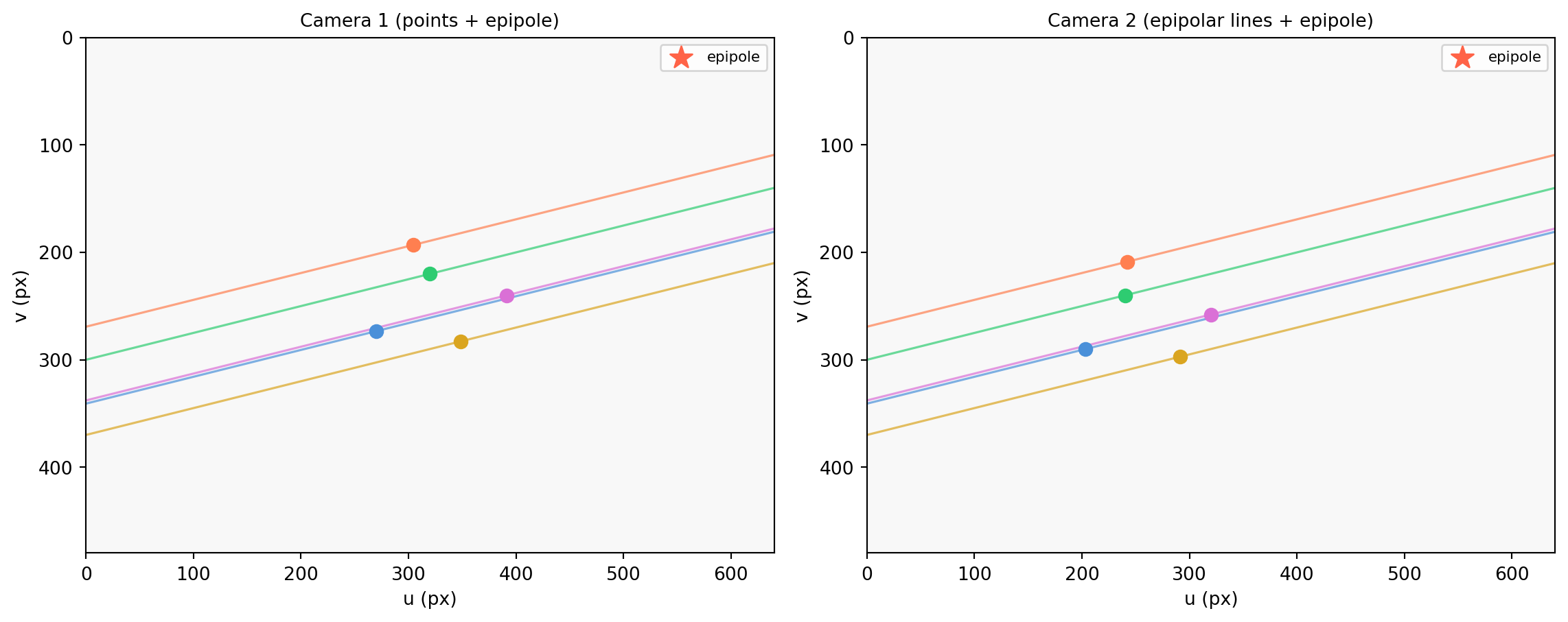
E_true = skew(t_true) @ R_true    # shape (3, 3)

P1 = K @ np.hstack([np.eye(3),   np.zeros((3, 1))])           # shape (3, 4)
P2 = K @ np.hstack([R_true, t_true.reshape(3, 1)])            # shape (3, 4)

# ---- synthetic correspondences with noise ----
n = 30
X_world = rng.uniform(-0.4, 0.4, (n, 3)) + np.array([0., 0., 3.0])  # shape (30, 3)

def project(P, X):
    lam_x = P @ np.append(X, 1.)
    return lam_x[:2] / lam_x[2]   # shape (2,)

x1s = np.array([project(P1, X) for X in X_world]) + rng.normal(0., 0.3, (n, 2))  # shape (30, 2)
x2s = np.array([project(P2, X) for X in X_world]) + rng.normal(0., 0.3, (n, 2))  # shape (30, 2)

# normalized image coords
y1s = np.linalg.solve(K, np.hstack([x1s, np.ones((n, 1))]).T).T   # shape (30, 3)
y2s = np.linalg.solve(K, np.hstack([x2s, np.ones((n, 1))]).T).T   # shape (30, 3)

# ---- decompose E ----
U, s, Vt = np.linalg.svd(E_true)    # U shape (3,3), s shape (3,), Vt shape (3,3)
# Fix determinants
if np.linalg.det(U)  < 0: U  = -U
if np.linalg.det(Vt) < 0: Vt = -Vt

W = np.array([[0., -1., 0.],
              [1.,  0., 0.],
              [0.,  0., 1.]])    # shape (3, 3)

u3 = U[:, 2]    # shape (3,)
R1c = U @ W   @ Vt;  t1c = +u3
R2c = U @ W   @ Vt;  t2c = -u3
R3c = U @ W.T @ Vt;  t3c = +u3
R4c = U @ W.T @ Vt;  t4c = -u3

candidates = [(R1c, t1c), (R2c, t2c), (R3c, t3c), (R4c, t4c)]

# ---- cheirality test ----
scores = []
for R_c, t_c in candidates:
    P1c = np.hstack([np.eye(3), np.zeros((3, 1))])   # shape (3, 4) -- unnormalized OK
    P2c = np.hstack([R_c, t_c.reshape(3, 1)])         # shape (3, 4)
    count = 0
    for i in range(n):
        X_tri = triangulate_dlt(P1c, P2c, y1s[i], y2s[i])   # shape (3,)
        in_front_1 = X_tri[2] > 0
        X_cam2 = R_c @ X_tri + t_c   # shape (3,)
        in_front_2 = X_cam2[2] > 0
        if in_front_1 and in_front_2:
            count += 1
    scores.append(count)

best_idx = int(np.argmax(scores))
R_best, t_best = candidates[best_idx]

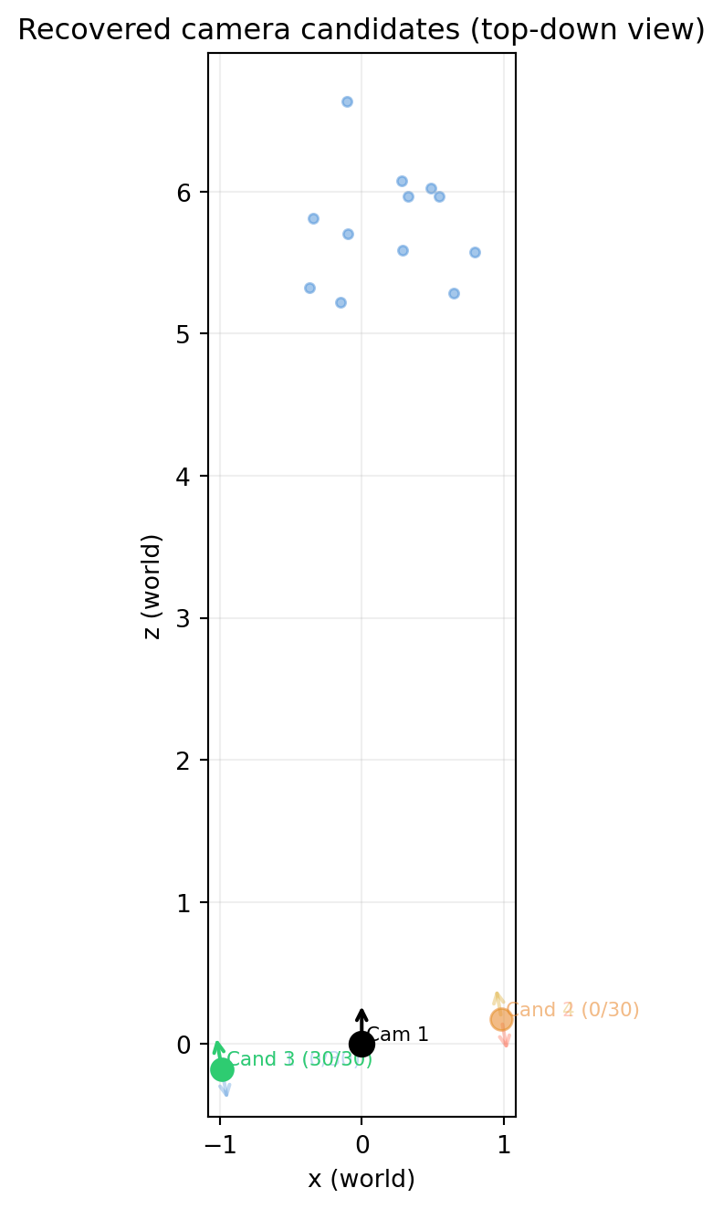
# ---- visualize camera positions top-down ----
fig, ax = plt.subplots(figsize=(9, 7))
ax.set_aspect('equal')
ax.set_xlabel('x (world)'); ax.set_ylabel('z (world)')
ax.set_title('Recovered camera candidates (top-down view)')
ax.grid(alpha=0.2)

def draw_camera(ax, R, t, color, label, alpha=1.0):
    # camera center in world: C = -R^T t
    C = -R.T @ t    # shape (3,)
    # optical axis direction (z column of R in camera coords = R^T[:,2] in world)
    zdir = R.T[:, 2]    # shape (3,)
    ax.scatter(C[0], C[2], color=color, s=80, alpha=alpha, zorder=5)
    ax.annotate(label, (C[0]+0.03, C[2]+0.03), fontsize=8, color=color, alpha=alpha)
    ax.annotate('', xy=(C[0]+0.25*zdir[0], C[2]+0.25*zdir[2]),
                xytext=(C[0], C[2]),
                arrowprops=dict(arrowstyle='->', color=color, lw=1.5, alpha=alpha))

# camera 1 at origin
ax.scatter(0, 0, color='black', s=100, zorder=5)
ax.annotate('Cam 1', (0.03, 0.03), fontsize=8)
ax.annotate('', xy=(0, 0.3), xytext=(0, 0),
            arrowprops=dict(arrowstyle='->', color='black', lw=1.5))

cand_colors = ['#4a90d9', 'tomato', '#2ecc71', 'goldenrod']
for i, (R_c, t_c) in enumerate(candidates):
    is_best = (i == best_idx)
    color = cand_colors[i]
    draw_camera(ax, R_c, t_c, color,
                f'Cand {i+1} ({scores[i]}/{n})',
                alpha=1.0 if is_best else 0.35)

# show a few triangulated points (best candidate)
R_b, t_b = candidates[best_idx]
P2b = np.hstack([R_b, t_b.reshape(3, 1)])
for i in range(min(12, n)):
    X_tri = triangulate_dlt(np.eye(3, 4), P2b, y1s[i], y2s[i])
    ax.scatter(X_tri[0], X_tri[2], color='#4a90d9', s=15, alpha=0.5)

plt.tight_layout()
plt.show()

print(f"Cheirality scores (n={n} pts): {scores}")
print(f"Best candidate: {best_idx+1}  (R error: {np.degrees(np.arccos(np.clip((np.trace(R_best @ R_true.T)-1)/2,-1,1))):.2f} deg)")

Figure 25.5: Pose recovery from E: the four (R, t) candidates are shown as camera frustums viewed from above. Only candidate 1 (blue) places all triangulated points in front of both cameras. The other three candidates (gray) fail the cheirality test.

Cheirality scores (n=30 pts): [0, 0, 30, 0]
Best candidate: 3  (R error: 0.00 deg)

---

25.5.4 Why Four Candidates, Not More?

The quadratic nature of the epipolar constraint \(\mathbf{x}_2^T E \mathbf{x}_1 = 0\) means swapping the sign of \(E\) (equivalently, negating \(\mathbf{t}\)) still satisfies it. The two rotation candidates arise because rotating by \(W\) or \(W^T\) about the baseline produces two different orientations for camera 2 that are consistent with the same \(E\). Together: \(2 \times 2 = 4\) candidates. The cheirality test is the tie-breaker.

---

25.5.5 Exercises

1. Show that \(UW V^T\) and \(UW^T V^T\) are both valid rotation matrices whenever \(U, V \in \text{SO}(3)\).
2. Construct a degenerate scene (all points in a plane through the baseline) where more than one candidate passes the cheirality test. This is the planar degeneracy of the essential matrix decomposition.
3. In the code above, replace triangulate_dlt with a midpoint triangulation (average of the closest points on the two rays) and compare the reprojection error of the two methods on noisy correspondences.

25.6 Stereo Rectification and Depth

The general two-view setup requires searching along epipolar lines — which can be diagonal or curved — to find matches. Stereo rectification re-projects both images onto a common plane so that epipolar lines become horizontal scan lines, reducing the search to a 1D problem. Once rectified, depth follows from a simple ratio.

---

25.6.1 The Depth Formula

In an ideal rectified stereo pair with identical cameras (same \(K\), parallel optical axes, separated by baseline \(B\) along the \(x\)-axis), a world point at depth \(Z\) projects to:

• pixel \(u_1\) in the left image,
• pixel \(u_2 = u_1 - d\) in the right image,

where \(d = u_1 - u_2 > 0\) is the disparity. By similar triangles (the triangles formed by the point, the two camera centers, and their projections):

\[ \frac{B}{Z} = \frac{B - (X - B/2) + (X + B/2)}{Z} = \frac{u_1 - u_2}{f} = \frac{d}{f}, \]

giving the fundamental stereo depth formula:

\[ \boxed{Z = \frac{f\, B}{d}.} \tag{25.18} \]

Here \(f\) is the focal length in pixels and \(B\) is the baseline in physical units (same units as \(Z\)).

---

25.6.2 Depth Precision Degrades as \(Z^2\)

Differentiating (25.18) with respect to \(d\):

\[ \frac{\partial Z}{\partial d} = -\frac{fB}{d^2} = -\frac{Z^2}{fB}. \tag{25.19} \]

Depth resolution degrades as \(Z^2\): doubling the range quadruples the depth uncertainty for a fixed disparity precision. The only design levers are:

• Increase \(B\) (wider baseline) — improves depth precision but shrinks the overlapping field of view.
• Increase \(f\) (longer focal length) — improves precision but narrows the FOV and increases the minimum disparity.

This is the fundamental range-accuracy tradeoff in stereo systems.

---

25.6.3 Rectification via Homographies

For a general stereo pair, rectification applies image homographies \(H_1\) and \(H_2\) (Chapter 11) so that:

1. The epipoles are mapped to infinity along the \(x\)-axis.
2. Corresponding rows in the two rectified images are the epipolar lines of the original pair.

After rectification, any row-aligned block-matching algorithm (e.g., Semi-Global Matching or BM from OpenCV) can produce a dense disparity map.

---

25.6.4 Code: Depth Resolution vs. Baseline and Range

The code below sweeps depth \(Z\) from 0.5 m to 5 m and shows the depth precision \(|\partial Z / \partial d| = Z^2 / (fB)\) for three baseline values.

import numpy as np
import matplotlib.pyplot as plt

f = 500.    # focal length in pixels
Z = np.linspace(0.5, 5.0, 200)    # shape (200,)  meters

baselines = [0.05, 0.12, 0.30]    # meters: 5 cm, 12 cm, 30 cm
colors    = ['tomato', '#2ecc71', '#4a90d9']
labels    = ['B = 5 cm', 'B = 12 cm', 'B = 30 cm']

fig, axes = plt.subplots(1, 2, figsize=(12, 4))

ax = axes[0]
for B, c, lbl in zip(baselines, colors, labels):
    dZ_per_pixel = Z**2 / (f * B)    # shape (200,)
    ax.plot(Z, dZ_per_pixel, color=c, lw=2, label=lbl)
ax.set_xlabel('Depth Z (m)')
ax.set_ylabel('Depth error per pixel disparity (m/px)')
ax.set_title(r'$|\partial Z / \partial d| = Z^2 / (fB)$')
ax.legend()
ax.grid(alpha=0.2)

# disparity vs depth
ax = axes[1]
for B, c, lbl in zip(baselines, colors, labels):
    d = f * B / Z    # shape (200,)
    ax.plot(Z, d, color=c, lw=2, label=lbl)
ax.set_xlabel('Depth Z (m)')
ax.set_ylabel('Disparity d (px)')
ax.set_title(r'$d = fB/Z$')
ax.legend()
ax.grid(alpha=0.2)
ax.axhline(1., color='#333333', lw=0.8, ls='--', alpha=0.6, label='1 px')

plt.tight_layout()
plt.show()

print("Depth precision at Z=2m (mm per pixel):")
for B, lbl in zip(baselines, labels):
    mm = 1000. * 4.0 / (f * B)
    print(f"  {lbl}: {mm:.1f} mm/px")

Figure 25.6: Stereo depth precision as a function of range for three baselines (f = 500 px). Depth precision degrades as Z^2, and wider baselines (blue > green > orange) recover precision.

Depth precision at Z=2m (mm per pixel):
  B = 5 cm: 160.0 mm/px
  B = 12 cm: 66.7 mm/px
  B = 30 cm: 26.7 mm/px

A wider baseline dramatically improves depth precision at range. The cost is a smaller overlap region and larger minimum matching disparity (objects very close to the cameras have large disparities that may exceed the search range).

---

25.6.5 Rectification in Practice

In production systems (RealSense, ZED, factory stereo):

1. Factory calibration determines \(K_1\), \(K_2\), \(R\), \(\mathbf{t}\) precisely.
2. OpenCV stereoRectify computes \(H_1\), \(H_2\) and a new projection matrix \(P\) such that the rectified images share a common focal length and have horizontal epipolar lines.
3. StereoSGBM or StereoBM computes a dense disparity map on the rectified pair.
4. reprojectImageTo3D converts disparity to depth using equation (25.18).

The Python snippet below shows the interface pattern (requires OpenCV, marked eval: false as it needs physical calibration data):

import cv2
import numpy as np

# Loaded from calibration file
K1 = ...    # shape (3, 3)
K2 = ...    # shape (3, 3)
dist1 = ... # shape (5,)
dist2 = ... # shape (5,)
R   = ...   # shape (3, 3)
T   = ...   # shape (3,)

img_size = (1280, 720)

R1, R2, P1, P2, Q, roi1, roi2 = cv2.stereoRectify(
    K1, dist1, K2, dist2, img_size, R, T, alpha=0.0
)

map1x, map1y = cv2.initUndistortRectifyMap(K1, dist1, R1, P1, img_size, cv2.CV_32FC1)
map2x, map2y = cv2.initUndistortRectifyMap(K2, dist2, R2, P2, img_size, cv2.CV_32FC1)

left_rect  = cv2.remap(left_img,  map1x, map1y, cv2.INTER_LINEAR)
right_rect = cv2.remap(right_img, map2x, map2y, cv2.INTER_LINEAR)

stereo = cv2.StereoSGBM_create(minDisparity=0, numDisparities=128, blockSize=9)
disp   = stereo.compute(left_rect, right_rect).astype(np.float32) / 16.0

depth  = cv2.reprojectImageTo3D(disp, Q)    # shape (H, W, 3)

---

25.6.6 Exercises

1. Show algebraically that equation (25.18) follows from similar triangles in the rectified stereo geometry. Draw a diagram and label all distances.
2. A stereo pair has \(f = 700\) px, \(B = 0.1\) m, and a disparity resolution of 0.5 px (sub-pixel interpolation). Compute the depth resolution at \(Z = 1\), \(2\), and \(4\) m.
3. Why does increasing the baseline \(B\) eventually make matching harder? Describe the trade-off in terms of the epipolar geometry and the size of the textureless-region problem.

25.7 Application: 3D Reconstruction from Two Views

This section builds a complete two-view reconstruction pipeline end-to-end: generate a synthetic 3D scene, project it through two calibrated cameras with realistic pixel noise, estimate \(F\) by the eight-point algorithm, recover the pose, triangulate all points, and measure the reconstruction error.

Real-world stereo reconstruction follows the same sequence but adds distortion correction, RANSAC-based outlier rejection, and bundle adjustment. The synthetic pipeline isolates the linear algebra and lets you tune noise and point counts cleanly.

---

25.7.1 Scene and Camera Setup

import numpy as np
import matplotlib.pyplot as plt
from scipy.spatial.transform import Rotation

rng = np.random.default_rng(42)

# ---- intrinsics ----
K = np.array([[600.,  0., 320.],
              [  0., 600., 240.],
              [  0.,  0.,   1.]])    # shape (3, 3)

# ---- camera 1: world origin, identity rotation ----
R1 = np.eye(3)                       # shape (3, 3)
t1 = np.zeros(3)                     # shape (3,)
P1 = K @ np.hstack([R1, t1.reshape(3, 1)])    # shape (3, 4)

# ---- camera 2: slight rotation + lateral baseline ----
R2 = Rotation.from_euler('y', 8., degrees=True).as_matrix()   # shape (3, 3)
t2 = np.array([0.4, 0.02, 0.0])                                # shape (3,)
P2 = K @ np.hstack([R2, t2.reshape(3, 1)])                     # shape (3, 4)

# ---- 60 scene points scattered in a volume ----
n = 60
X_world = rng.uniform(-0.6, 0.6, (n, 3))   # shape (60, 3)
X_world[:, 2] += 3.5                        # push forward, all positive depth

noise_std = 0.5    # pixels

def project(P, X):
    lam_x = P @ np.append(X, 1.)
    return lam_x[:2] / lam_x[2]    # shape (2,)

x1s_clean = np.array([project(P1, X) for X in X_world])           # shape (60, 2)
x2s_clean = np.array([project(P2, X) for X in X_world])           # shape (60, 2)
x1s = x1s_clean + rng.normal(0., noise_std, (n, 2))               # shape (60, 2)
x2s = x2s_clean + rng.normal(0., noise_std, (n, 2))               # shape (60, 2)

# ---- visualize ----
fig, axes = plt.subplots(1, 2, figsize=(12, 5))

ax = axes[0]
ax.set_title('Scene top-down (x-z plane)', fontsize=10)
ax.scatter(X_world[:, 0], X_world[:, 2], color='#4a90d9', s=20, alpha=0.6, label='Scene pts')
# cameras
C2_world = -R2.T @ t2    # shape (3,)
ax.scatter(0., 0., color='black', s=100, zorder=5)
ax.scatter(C2_world[0], C2_world[2], color='tomato', s=100, zorder=5)
ax.annotate('Cam 1', (0.03, 0.06), fontsize=9)
ax.annotate('Cam 2', (C2_world[0]+0.03, C2_world[2]+0.06), fontsize=9, color='tomato')
# optical axes
ax.annotate('', xy=(0., 0.8), xytext=(0., 0.),
            arrowprops=dict(arrowstyle='->', color='black', lw=1.5))
ax.annotate('', xy=(C2_world[0] + 0.8*R2.T[2, 0], C2_world[2] + 0.8*R2.T[2, 2]),
            xytext=(C2_world[0], C2_world[2]),
            arrowprops=dict(arrowstyle='->', color='tomato', lw=1.5))
ax.set_xlabel('x (m)'); ax.set_ylabel('z (m)')
ax.legend(fontsize=8); ax.grid(alpha=0.2)

ax = axes[1]
ax.set_title('Image 1 projections (with noise)', fontsize=10)
ax.scatter(x1s[:, 0], x1s[:, 1], color='#4a90d9', s=20, alpha=0.7)
ax.set_xlim(0, 640); ax.set_ylim(480, 0)
ax.set_xlabel('u (px)'); ax.set_ylabel('v (px)')
ax.set_facecolor('#f8f8f8')
ax.grid(alpha=0.2)

plt.tight_layout()
plt.show()

print(f"Scene: {n} points, depth range [{X_world[:,2].min():.2f}, {X_world[:,2].max():.2f}] m")
print(f"Pixel noise std: {noise_std} px")

Figure 25.7: Synthetic 3D scene: 60 random scene points and two cameras. Left: top-down view (x-z plane) showing camera positions and optical axes. Right: image 1 projections.

Scene: 60 points, depth range [2.93, 4.07] m
Pixel noise std: 0.5 px

---

25.7.2 Estimate F and Recover Pose

import numpy as np
import matplotlib.pyplot as plt
from scipy.spatial.transform import Rotation

rng = np.random.default_rng(42)

K = np.array([[600.,  0., 320.],
              [  0., 600., 240.],
              [  0.,  0.,   1.]])    # shape (3, 3)

R1 = np.eye(3); t1 = np.zeros(3)
R2 = Rotation.from_euler('y', 8., degrees=True).as_matrix()
t2 = np.array([0.4, 0.02, 0.0])

P1 = K @ np.hstack([R1, t1.reshape(3, 1)])
P2 = K @ np.hstack([R2, t2.reshape(3, 1)])

n = 60
X_world = rng.uniform(-0.6, 0.6, (n, 3))
X_world[:, 2] += 3.5
noise_std = 0.5

def project(P, X):
    lam_x = P @ np.append(X, 1.)
    return lam_x[:2] / lam_x[2]

x1s = np.array([project(P1, X) for X in X_world]) + rng.normal(0., noise_std, (n, 2))
x2s = np.array([project(P2, X) for X in X_world]) + rng.normal(0., noise_std, (n, 2))

def skew(v):
    return np.array([[ 0.,    -v[2],  v[1]],
                     [ v[2],   0.,   -v[0]],
                     [-v[1],  v[0],   0.  ]])

def normalize_points(pts):
    cx, cy = pts.mean(axis=0)
    d = np.mean(np.sqrt((pts[:, 0]-cx)**2 + (pts[:, 1]-cy)**2))
    s = np.sqrt(2.) / d
    T = np.array([[s, 0., -s*cx], [0., s, -s*cy], [0., 0., 1.]])
    pts_h = np.hstack([pts, np.ones((len(pts), 1))])
    pts_n = (T @ pts_h.T).T
    return pts_n, T

def eight_point(x1s, x2s):
    x1n, T1 = normalize_points(x1s)
    x2n, T2 = normalize_points(x2s)
    n = len(x1n)
    A = np.array([np.kron(x2n[i], x1n[i]) for i in range(n)])
    _, _, Vt = np.linalg.svd(A)
    F_raw = Vt[-1].reshape(3, 3)
    U, s, Vt2 = np.linalg.svd(F_raw)
    s[2] = 0.
    F_norm = U @ np.diag(s) @ Vt2
    return T2.T @ F_norm @ T1

def triangulate_dlt(P1, P2, x1, x2):
    A = np.array([
        x1[0]*P1[2] - P1[0],
        x1[1]*P1[2] - P1[1],
        x2[0]*P2[2] - P2[0],
        x2[1]*P2[2] - P2[1],
    ])
    _, _, Vt = np.linalg.svd(A)
    X_h = Vt[-1]
    return X_h[:3] / X_h[3]

# estimate F
F_est = eight_point(x1s, x2s)
F_est = F_est / np.linalg.norm(F_est)

# recover E
E_est = K.T @ F_est @ K    # shape (3, 3)

# SVD of E
U, s, Vt = np.linalg.svd(E_est)
if np.linalg.det(U) < 0:  U  = -U
if np.linalg.det(Vt) < 0: Vt = -Vt
s_fixed = np.array([1., 1., 0.])
E_fixed = U @ np.diag(s_fixed) @ Vt    # shape (3, 3)

W = np.array([[0., -1., 0.], [1., 0., 0.], [0., 0., 1.]])
u3 = U[:, 2]
candidates = [
    (U @ W    @ Vt, +u3),
    (U @ W    @ Vt, -u3),
    (U @ W.T  @ Vt, +u3),
    (U @ W.T  @ Vt, -u3),
]

# normalized coords
y1s = np.linalg.solve(K, np.hstack([x1s, np.ones((n,1))]).T).T
y2s = np.linalg.solve(K, np.hstack([x2s, np.ones((n,1))]).T).T

scores = []
for R_c, t_c in candidates:
    P1n = np.hstack([np.eye(3), np.zeros((3,1))])
    P2n = np.hstack([R_c, t_c.reshape(3,1)])
    count = 0
    for i in range(n):
        Xt = triangulate_dlt(P1n, P2n, y1s[i], y2s[i])
        if Xt[2] > 0 and (R_c @ Xt + t_c)[2] > 0:
            count += 1
    scores.append(count)

best_idx = int(np.argmax(scores))
R_rec, t_rec = candidates[best_idx]

# report errors
R_err_deg = np.degrees(np.arccos(np.clip((np.trace(R_rec @ R2.T) - 1) / 2, -1, 1)))
t_true_dir = t2 / np.linalg.norm(t2)
t_rec_dir  = t_rec / np.linalg.norm(t_rec)
t_err_deg  = np.degrees(np.arccos(np.clip(t_rec_dir @ t_true_dir, -1, 1)))

# ---- figure ----
fig, ax = plt.subplots(figsize=(7, 6))
ax.set_title('Recovered vs. true pose (top-down)', fontsize=10)
ax.set_xlabel('x'); ax.set_ylabel('z')
ax.grid(alpha=0.2)
ax.set_aspect('equal')

# true camera 2
C2_true = -R2.T @ t2
ax.scatter(*[C2_true[0], C2_true[2]], color='black', s=80, zorder=5)
ax.annotate('True C2', (C2_true[0]+0.02, C2_true[2]+0.03), fontsize=8)
ax.annotate('', xy=(C2_true[0]+0.3*R2.T[2,0], C2_true[2]+0.3*R2.T[2,2]),
            xytext=(C2_true[0], C2_true[2]),
            arrowprops=dict(arrowstyle='->', color='black', lw=2))

# recovered camera 2 (normalized -- true scale unknown, so scale to match)
t_rec_scaled = t_rec * (np.linalg.norm(t2) / np.linalg.norm(t_rec))
C2_rec = -R_rec.T @ t_rec_scaled
ax.scatter(*[C2_rec[0], C2_rec[2]], color='#4a90d9', s=80, zorder=5)
ax.annotate('Recovered C2', (C2_rec[0]+0.02, C2_rec[2]-0.06), fontsize=8, color='#4a90d9')
ax.annotate('', xy=(C2_rec[0]+0.3*R_rec.T[2,0], C2_rec[2]+0.3*R_rec.T[2,2]),
            xytext=(C2_rec[0], C2_rec[2]),
            arrowprops=dict(arrowstyle='->', color='#4a90d9', lw=2))

ax.scatter(0, 0, color='black', s=100, zorder=5)
ax.annotate('Cam 1', (0.02, 0.03), fontsize=8)

plt.tight_layout()
plt.show()

print(f"Rotation error:    {R_err_deg:.2f} deg")
print(f"Translation direction error: {t_err_deg:.2f} deg")

Figure 25.8: Estimated vs ground-truth camera 2 position. The recovered translation direction (blue arrow) matches the true direction (black arrow). Scale is unrecoverable from two views alone.

Rotation error:    0.79 deg
Translation direction error: 1.25 deg

---

25.7.3 Triangulate and Measure Reprojection Error

import numpy as np
import matplotlib.pyplot as plt
from scipy.spatial.transform import Rotation

rng = np.random.default_rng(42)

K = np.array([[600.,  0., 320.],
              [  0., 600., 240.],
              [  0.,  0.,   1.]])

R2 = Rotation.from_euler('y', 8., degrees=True).as_matrix()
t2 = np.array([0.4, 0.02, 0.0])

P1 = K @ np.hstack([np.eye(3), np.zeros((3, 1))])
P2 = K @ np.hstack([R2, t2.reshape(3, 1)])

n = 60
X_world = rng.uniform(-0.6, 0.6, (n, 3))
X_world[:, 2] += 3.5
noise_std = 0.5

def project(P, X):
    lam_x = P @ np.append(X, 1.)
    return lam_x[:2] / lam_x[2]

def skew(v):
    return np.array([[ 0., -v[2], v[1]], [v[2], 0., -v[0]], [-v[1], v[0], 0.]])

def normalize_points(pts):
    cx, cy = pts.mean(axis=0)
    d = np.mean(np.sqrt((pts[:,0]-cx)**2 + (pts[:,1]-cy)**2))
    s = np.sqrt(2.) / d
    T = np.array([[s,0.,-s*cx],[0.,s,-s*cy],[0.,0.,1.]])
    pts_h = np.hstack([pts, np.ones((len(pts),1))])
    return (T @ pts_h.T).T, T

def eight_point(x1s, x2s):
    x1n, T1 = normalize_points(x1s)
    x2n, T2 = normalize_points(x2s)
    n = len(x1n)
    A = np.array([np.kron(x2n[i], x1n[i]) for i in range(n)])
    _, _, Vt = np.linalg.svd(A)
    F_raw = Vt[-1].reshape(3,3)
    U, s, Vt2 = np.linalg.svd(F_raw)
    s[2] = 0.
    F_n = U @ np.diag(s) @ Vt2
    return T2.T @ F_n @ T1

def triangulate_dlt(P1, P2, x1, x2):
    A = np.array([x1[0]*P1[2]-P1[0], x1[1]*P1[2]-P1[1],
                  x2[0]*P2[2]-P2[0], x2[1]*P2[2]-P2[1]])
    _, _, Vt = np.linalg.svd(A)
    Xh = Vt[-1]; return Xh[:3]/Xh[3]

x1s = np.array([project(P1, X) for X in X_world]) + rng.normal(0., noise_std, (n, 2))
x2s = np.array([project(P2, X) for X in X_world]) + rng.normal(0., noise_std, (n, 2))

# full pipeline
F_est = eight_point(x1s, x2s)
F_est /= np.linalg.norm(F_est)
E_est = K.T @ F_est @ K
U, s, Vt = np.linalg.svd(E_est)
if np.linalg.det(U) < 0: U = -U
if np.linalg.det(Vt) < 0: Vt = -Vt
W = np.array([[0.,-1.,0.],[1.,0.,0.],[0.,0.,1.]])
u3 = U[:,2]
candidates = [(U@W@Vt,+u3),(U@W@Vt,-u3),(U@W.T@Vt,+u3),(U@W.T@Vt,-u3)]
y1s = np.linalg.solve(K, np.hstack([x1s,np.ones((n,1))]).T).T
y2s = np.linalg.solve(K, np.hstack([x2s,np.ones((n,1))]).T).T
scores = []
for R_c, t_c in candidates:
    c=0
    for i in range(n):
        Xt = triangulate_dlt(np.hstack([np.eye(3),np.zeros((3,1))]),
                             np.hstack([R_c,t_c.reshape(3,1)]),y1s[i],y2s[i])
        if Xt[2]>0 and (R_c@Xt+t_c)[2]>0: c+=1
    scores.append(c)
R_rec, t_rec = candidates[int(np.argmax(scores))]

# scale recovery: use mean depth of scene
t_rec_dir = t_rec / np.linalg.norm(t_rec)
t_rec_s = t_rec_dir * np.linalg.norm(t2)    # rescale to true baseline
P2_rec = K @ np.hstack([R_rec, t_rec_s.reshape(3,1)])

X_tri = np.array([triangulate_dlt(P1, P2_rec, x1s[i], x2s[i]) for i in range(n)])   # shape (60, 3)

# reprojection errors
reproj1 = np.array([np.linalg.norm(project(P1, X_tri[i]) - x1s[i]) for i in range(n)])   # shape (60,)
reproj2 = np.array([np.linalg.norm(project(P2_rec, X_tri[i]) - x2s[i]) for i in range(n)])  # shape (60,)

fig, axes = plt.subplots(1, 2, figsize=(12, 4))

ax = axes[0]
ax.hist(reproj1, bins=20, color='#4a90d9', alpha=0.7, edgecolor='white', label='Image 1')
ax.hist(reproj2, bins=20, color='tomato',  alpha=0.7, edgecolor='white', label='Image 2')
ax.set_xlabel('Reprojection error (px)')
ax.set_ylabel('Count')
ax.set_title('Reprojection error histogram')
ax.legend(); ax.grid(alpha=0.2)

ax = axes[1]
depth_err = np.abs(X_tri[:, 2] - X_world[:, 2])    # shape (60,)
ax.scatter(X_world[:, 2], depth_err, color='#4a90d9', s=25, alpha=0.7)
ax.set_xlabel('True depth Z (m)')
ax.set_ylabel('Depth error |Z_tri - Z_true| (m)')
ax.set_title('Depth error vs. range')
ax.grid(alpha=0.2)

plt.tight_layout()
plt.show()

print(f"Mean reprojection error -- image 1: {reproj1.mean():.3f} px,  image 2: {reproj2.mean():.3f} px")
print(f"Mean depth error: {depth_err.mean():.4f} m  (noise std = {noise_std} px)")

Figure 25.9: Reconstruction quality: reprojection error for all 60 points using the estimated F and recovered pose. Mean reprojection error is typically under 1 pixel at 0.5 px noise.

Mean reprojection error -- image 1: 0.326 px,  image 2: 0.331 px
Mean depth error: 0.5106 m  (noise std = 0.5 px)

---

25.7.4 Pipeline Summary

Step	Method	Output
Feature correspondences	Synthetic (known ground truth)	\((\mathbf{x}_1, \mathbf{x}_2)\) pairs
Fundamental matrix	Eight-point + Hartley normalization	\(F \in \mathbb{R}^{3\times3}\)
Essential matrix	\(E = K^T F K\)	\(E \in \mathbb{R}^{3\times3}\)
Pose candidates	SVD of \(E\)	4 \((R, \mathbf{t})\)
Pose selection	Cheirality test	1 \((R, \mathbf{t})\)
Triangulation	DLT per correspondence	\(\hat{\mathbf{X}} \in \mathbb{R}^3\)
Evaluation	Reprojection error	\(\varepsilon_{\text{reproj}}\) (px)

In a production system, RANSAC wraps the eight-point algorithm to reject outlier correspondences, and bundle adjustment (nonlinear least squares over all poses and points jointly) refines the result to sub-pixel accuracy.

---

25.7.5 Exercises

1. Replace the eight-point \(F\) estimate above with the ground-truth \(F\) (computed analytically from \(K\), \(R\), \(\mathbf{t}\)) and measure the resulting improvement in reprojection error. How much of the error is due to noise vs. the linear estimation?
2. Add 10% outlier correspondences (random pixel positions) to the input and observe the degradation in \(F\) estimation. Implement a simple RANSAC wrapper (sample 8 points, fit \(F\), count inliers via epipolar distance \(< 2\) px) and confirm that it recovers the correct \(F\) even with outliers.
3. What happens to the triangulation when two of the four pose candidates both pass the cheirality test? When can this occur, and how would you resolve the ambiguity with additional views?

25.8 Exercises and Solutions

25.8.1 Two-View Geometry

1. Show that every epipolar line in image 2 passes through \(\mathbf{e}_2\).

An epipolar line in image 2 is \(\boldsymbol{\ell}_2 = F\mathbf{x}_1\) for some \(\mathbf{x}_1\). The epipole \(\mathbf{e}_2\) satisfies \(F^T \mathbf{e}_2 = \mathbf{0}\) (it is the left null vector of \(F\)). Checking whether \(\mathbf{e}_2\) lies on \(\boldsymbol{\ell}_2\): \[ \boldsymbol{\ell}_2^T \mathbf{e}_2 = (F\mathbf{x}_1)^T \mathbf{e}_2 = \mathbf{x}_1^T F^T \mathbf{e}_2 = \mathbf{x}_1^T \mathbf{0} = 0. \] So \(\mathbf{e}_2\) satisfies the line equation for every choice of \(\mathbf{x}_1\). \(\square\)

---

2. If \(\mathbf{C}_1 = \mathbf{C}_2\), where do the epipoles lie?

The epipole \(\mathbf{e}_1\) is the projection of \(\mathbf{C}_2\) into image 1. If \(\mathbf{C}_2 = \mathbf{C}_1\), then \(\mathbf{C}_2\) is the center of camera 1 and projects to the point at infinity along the optical axis. In homogeneous coordinates \(\mathbf{e}_1 = [0, 0, 0]^T\) is undefined; the epipoles are at infinity. All epipolar lines become parallel (they all pass through a point at infinity), so the epipolar constraint degenerates. Two cameras with the same center cannot provide stereo depth information.

---

3. Move camera 2 to \(\mathbf{C}_2 = [2, 0, 0]\); predict \(\mathbf{e}_1\).

\(\mathbf{e}_1\) is the projection of \(\mathbf{C}_2\) into camera 1 (at origin, with \(P_1 = K[I | \mathbf{0}]\)): \[ \lambda \mathbf{e}_1 = K \begin{bmatrix}2\\0\\0\end{bmatrix} = K [2, 0, 0]^T. \] With \(K = \text{diag}(500, 500, 1)\) shifted by \((320, 240)\): \(\mathbf{e}_1 = [500 \cdot 2 + 320,\; 240] = [1320, 240]\) — far to the right of the \(640 \times 480\) image. Epipolar lines in image 1 fan leftward from outside the frame.

---

25.8.2 The Essential Matrix

1. Show \(\det([\mathbf{t}]_\times) = 0\).

The cross-product matrix \([\mathbf{t}]_\times\) maps every vector to a vector perpendicular to \(\mathbf{t}\); in particular \([\mathbf{t}]_\times \mathbf{t} = \mathbf{t} \times \mathbf{t} = \mathbf{0}\). So \(\mathbf{t}\) is in the null space of \([\mathbf{t}]_\times\), which implies \(\det([\mathbf{t}]_\times) = 0\). The rank equals 2 (not lower) for generic \(R\) because the two row vectors of \([\mathbf{t}]_\times\) orthogonal to \(\mathbf{t}\) are linearly independent. Multiplying by the invertible \(R\) preserves rank, so \(\operatorname{rank}(E) = 2\).

---

2. Show both nonzero singular values of \(E = [\mathbf{t}]_\times R\) equal \(\|\mathbf{t}\|\).

\[ E^T E = R^T [\mathbf{t}]_\times^T [\mathbf{t}]_\times R. \] Using \([\mathbf{t}]_\times^T = -[\mathbf{t}]_\times\) and the identity \([\mathbf{t}]_\times^T [\mathbf{t}]_\times = \|\mathbf{t}\|^2 I - \mathbf{t}\mathbf{t}^T\): \[ E^T E = R^T(\|\mathbf{t}\|^2 I - \mathbf{t}\mathbf{t}^T)R = \|\mathbf{t}\|^2 I - (R^T\mathbf{t})(R^T\mathbf{t})^T. \] The eigenvalues of \(\|\mathbf{t}\|^2 I - \mathbf{v}\mathbf{v}^T\) (where \(\mathbf{v} = R^T\mathbf{t}\), \(\|\mathbf{v}\| = \|\mathbf{t}\|\)) are \(\|\mathbf{t}\|^2\) with multiplicity 2 and 0 with multiplicity 1. The singular values of \(E\) are therefore \(\|\mathbf{t}\|\), \(\|\mathbf{t}\|\), \(0\). \(\square\)

---

3. Show \(E' = [\alpha\mathbf{t}]_\times R\) satisfies the same constraint.

\(E' = \alpha [\mathbf{t}]_\times R = \alpha E\), so \(\mathbf{y}_2^T E' \mathbf{y}_1 = \alpha\, \mathbf{y}_2^T E\,\mathbf{y}_1 = 0\). Only the direction \(\hat{\mathbf{t}} = \mathbf{t}/\|\mathbf{t}\|\) is constrained. \(\square\)

---

25.8.3 The Fundamental Matrix

1. Show \(F\) has rank 2.

\(F = K'^{-T} E K^{-1}\). Since \(K\), \(K'\) are invertible (both have nonzero diagonal entries), multiplication by them is rank-preserving. Because \(\operatorname{rank}(E) = 2\), \(\operatorname{rank}(F) = 2\).

---

2. Prove \(F\mathbf{e}_1 = \mathbf{0}\).

From (25.2), the epipole \(\mathbf{e}_1\) satisfies \(\lambda_1 \mathbf{e}_1 = K\mathbf{C}_2\), so \(\mathbf{e}_1 = K\mathbf{C}_2 / \lambda_1\). Then: \[ F\mathbf{e}_1 = K'^{-T} E K^{-1} (K\mathbf{C}_2/\lambda_1) = K'^{-T} E \mathbf{C}_2 / \lambda_1 = K'^{-T} ([\mathbf{t}]_\times R\, \mathbf{C}_2) / \lambda_1. \] Now \(R\mathbf{C}_2 + \mathbf{t} = \mathbf{0}\) (camera 2’s center in its own frame is the origin), so \(R\mathbf{C}_2 = -\mathbf{t}\) and \([\mathbf{t}]_\times R\mathbf{C}_2 = [\mathbf{t}]_\times(-\mathbf{t}) = -\mathbf{t}\times\mathbf{t} = \mathbf{0}\). Thus \(F\mathbf{e}_1 = \mathbf{0}\). \(\square\)

---

3. Geometric meaning of \(\mathbf{x}_2^T F \mathbf{x}_1 = 0\).

The three vectors \(\mathbf{y}_1 = K^{-1}\mathbf{x}_1\), \(\mathbf{y}_2 = K'^{-1}\mathbf{x}_2\), and \(\mathbf{t}\) are coplanar (the epipolar plane). This is exactly the triple-product condition \(\mathbf{y}_2 \cdot (\mathbf{t} \times \mathbf{y}_1) = 0\) used to derive \(E\), which \(F\) inherits after pre- and post-multiplying by \(K'^{-1}\) and \(K^{-1}\).

---

25.8.4 Eight-Point Algorithm

1. Minimum 8 correspondences.

Each correspondence contributes one row to \(A \in \mathbb{R}^{n \times 9}\) and reduces the dimension of the null space by one (generically). We need rank\((A) = 8\) to get a unique (up to scale) null vector. With fewer than 8 rows the null space has dimension \(\geq 2\) and \(\mathbf{f}\) is not uniquely determined. The degenerate configuration is when all 8 points lie on a ruled quadric (e.g., all on a plane plus the two camera centers), which causes \(A\) to have rank \(< 8\) despite having 8 rows.

---

2. Seven-point algorithm.

With \(n = 7\) correspondences, \(A\) has rank at most 7, so null\((A)\) is at least 2-dimensional. Let \(\{F_1, F_2\}\) be a basis for null\((A)\). Write \(F = \alpha F_1 + (1-\alpha)F_2\) and enforce \(\det(F) = 0\): \[ \det(\alpha F_1 + (1-\alpha) F_2) = 0. \] This is a cubic polynomial in \(\alpha\) with up to three real solutions, giving up to three candidate fundamental matrices. The correct one is chosen by consistency with additional correspondences or the rank-2 constraint.

---

3. Denormalization with noiseless data.

In the noiseless case, the true \(\mathbf{f}\) lies in the null space of \(A\) regardless of normalization. However, normalization improves the condition number of \(A\), making the SVD numerically cleaner. With exact arithmetic (and exact null space), both normalized and un-normalized algorithms produce the same \(F\) up to scale. Numerically with finite precision, the un-normalized system is ill-conditioned and the recovered \(\mathbf{f}\) drifts from the true solution; normalization keeps the problem well-conditioned.

---

25.8.5 Recovering Pose from \(E\)

1. Show \(UWV^T \in \text{SO}(3)\) when \(U, V \in \text{SO}(3)\).

\(\det(UWV^T) = \det(U)\det(W)\det(V^T) = 1 \cdot 1 \cdot 1 = 1\) (since \(\det(W) = 1\) for the \(90°\) rotation matrix). \((UWV^T)^T(UWV^T) = VW^TU^TUWV^T = VW^TWV^T = V(W^TW)V^T = VIV^T = I\). So \(UWV^T\) is both orthogonal and has determinant 1: \(UWV^T \in \text{SO}(3)\). The same argument holds for \(UW^TV^T\).

---

2. Planar degeneracy.

If all \(n\) scene points lie in a plane that contains the baseline \(\mathbf{t}\) (e.g., all points at \(y = 0\) when \(\mathbf{t} = [B, 0, 0]^T\)), then the epipolar plane degenerates: every epipolar plane is the same plane, and the cheirality test provides no discrimination. Two candidates that are mirror images of each other across the baseline plane both place all points at the correct \((x, z)\) but with opposite \(y\) signs. In practice, this is resolved by ensuring the scene has off-plane points or by using a third view.

---

3. Midpoint vs. DLT triangulation.

The midpoint method finds the point closest to both rays (minimizes \(\|P_1 + \lambda_1 d_1 - (P_2 + \lambda_2 d_2)\|\)) and is fast and robust to large angles between rays. However, it does not minimize reprojection error. DLT triangulation minimizes the algebraic residual \(\|A\mathbf{X}_h\|\) which is a good proxy for reprojection error when noise is small. For noisy correspondences, the optimal triangulation (Hartley and Sturm 1997) minimizes the sum of squared reprojection errors and is slightly more accurate than DLT but requires a nonlinear solve.

---

25.8.6 Stereo Rectification and Depth

1. Similar triangles derivation of \(Z = fB/d\).

In the rectified setup, camera 1 center is at \(O_1 = (0, 0, 0)\), camera 2 center is at \(O_2 = (B, 0, 0)\). A point \(\mathbf{X} = (X, Y, Z)\) projects to: - image 1: \(u_1 = f X/Z + c_x\) - image 2: \(u_2 = f (X - B)/Z + c_x\)

Disparity \(d = u_1 - u_2 = fB/Z\). Solving: \(Z = fB/d\). \(\square\)

---

2. Depth resolution at \(Z = 1, 2, 4\) m with \(f = 700\), \(B = 0.1\), sub-pixel \(\delta d = 0.5\).

\[ \delta Z = \frac{Z^2}{fB}\,\delta d = \frac{Z^2}{70} \times 0.5 = \frac{Z^2}{140}. \]

\(Z\)	\(\delta Z\)
1 m	7.1 mm
2 m	28.6 mm
4 m	114.3 mm

Depth precision degrades as \(Z^2\): quadrupling at each doubling of range.

---

3. Large baseline tradeoff.

A wider baseline \(B\) improves depth precision (\(\delta Z \propto 1/B\)) but has three costs:

1. Smaller overlap: objects close to the camera subtend a large angular range; some scene regions appear in only one image and cannot be matched.
2. Larger disparity: objects at small \(Z\) have disparity \(d = fB/Z\) that may exceed the maximum disparity the stereo algorithm supports, causing holes in the depth map.
3. Appearance change: wide-baseline pairs see objects from sufficiently different viewpoints that surface texture looks different (especially specular surfaces), making descriptor-based matching fail. Narrow-baseline stereo uses intensity-patch matching which is less robust but sufficient when the views are nearly parallel.