26 Appendix A: Python / NumPy / SciPy / OpenCV Quick Reference

26.1 NumPy Array Essentials

This section is a compact reference for the NumPy patterns used throughout the book. For a complete treatment see the NumPy documentation at https://numpy.org/doc/.

26.1.1 Array Creation

Expression	Shape	Notes
`np.array([1.0, 2.0, 3.0])`	`(3,)`	Dtype inferred; use float literals to get float64
`np.zeros((m, n))`	`(m, n)`	Default dtype float64
`np.ones((m, n))`	`(m, n)`
`np.eye(n)`	`(n, n)`	`np.eye(m, n, k)` for rectangular or off-diagonal
`np.arange(start, stop, step)`	`(k,)`	Prefer `linspace` for floats
`np.linspace(a, b, num)`	`(num,)`	Inclusive at both ends
`np.full((m, n), val)`	`(m, n)`	Constant fill
`np.diag(v)`	`(n, n)`	Diagonal matrix from vector; or extract diagonal from matrix
`np.block([[A, B], [C, D]])`	varies	Block matrix assembly
`rng.standard_normal((m, n))`	`(m, n)`	Always `rng = np.random.default_rng(seed)`
`rng.integers(0, high, size=(m, n))`	`(m, n)`	`high` is exclusive

import numpy as np

rng = np.random.default_rng(0)

v   = np.array([1.0, 2.0, 3.0])      # shape (3,)
A   = np.zeros((3, 4))                # shape (3, 4)
I3  = np.eye(3)                       # shape (3, 3)
x   = np.linspace(0.0, 1.0, 5)       # shape (5,)
M   = rng.standard_normal((3, 3))    # shape (3, 3)
D   = np.diag(np.array([1.0, 2.0, 3.0]))   # shape (3, 3)

# Block matrix: [[I, 0], [0, 2I]]
blk = np.block([[np.eye(2), np.zeros((2, 2))],
                [np.zeros((2, 2)), 2.0 * np.eye(2)]])   # shape (4, 4)

print("v  :", v.shape, v.dtype)
print("A  :", A.shape, A.dtype)
print("I3 :", I3.shape, I3.dtype)
print("x  :", x)
print("M  :\n", M.round(3))
print("blk diagonal:", blk.diagonal())

v  : (3,) float64
A  : (3, 4) float64
I3 : (3, 3) float64
x  : [0.   0.25 0.5  0.75 1.  ]
M  :
 [[ 0.126 -0.132  0.64 ]
 [ 0.105 -0.536  0.362]
 [ 1.304  0.947 -0.704]]
blk diagonal: [1. 1. 2. 2.]

26.1.2 Inspecting Arrays

Attribute	Meaning
`.shape`	Tuple of dimension sizes
`.ndim`	Number of axes
`.dtype`	Element data type
`.size`	Total element count
`.itemsize`	Bytes per element
`.nbytes`	Total bytes (`size * itemsize`)
`.T`	Transposed view (no copy for 2-D)

import numpy as np

A = np.eye(4, dtype=np.float32)    # shape (4, 4)
print(f"shape={A.shape}  ndim={A.ndim}  dtype={A.dtype}")
print(f"size={A.size}  itemsize={A.itemsize} bytes  nbytes={A.nbytes} bytes")

shape=(4, 4)  ndim=2  dtype=float32
size=16  itemsize=4 bytes  nbytes=64 bytes

26.1.3 Core Operations

Operation	Syntax	Notes
Matrix multiply	`A @ B`	Use `@`; never `np.dot` for matrices
Element-wise multiply	`A * B`	Requires broadcastable shapes
Scalar multiply	`3.0 * A`	Returns a new array
Transpose	`A.T`	View; `.conj().T` for Hermitian
Solve \(Ax = b\)	`np.linalg.solve(A, b)`	Square `A` only
Least-squares	`np.linalg.lstsq(A, b, rcond=None)`	Returns `(x, residuals, rank, sv)`
Sum along axis	`A.sum(axis=0)`	Reduces that axis
Mean along axis	`A.mean(axis=1)`
Clip	`np.clip(A, lo, hi)`

import numpy as np

rng = np.random.default_rng(1)
A = rng.standard_normal((3, 3))    # shape (3, 3)
b = rng.standard_normal((3,))      # shape (3,)

x   = np.linalg.solve(A, b)        # shape (3,)
res = np.linalg.norm(A @ x - b)
print(f"||Ax - b|| = {res:.2e}")

B      = rng.standard_normal((3, 3))    # shape (3, 3)
C_mat  = A @ B                          # shape (3, 3)  matrix product
C_elem = A * B                          # shape (3, 3)  Hadamard product
print("matmul == elemwise:", np.allclose(C_mat, C_elem))

||Ax - b|| = 6.09e-16
matmul == elemwise: False

26.1.4 Shape Manipulation

Function	Result
`A.reshape(m, n)`	New shape; total element count unchanged
`A.ravel()`	Flatten to 1-D, C order (may return a view)
`A.flatten()`	Flatten to 1-D, always copies
`A.squeeze()`	Remove all size-1 axes
`A[np.newaxis, :]`	Insert size-1 axis at front
`np.expand_dims(A, axis)`	Insert size-1 axis at position
`np.concatenate([A, B], axis)`	Join along existing axis
`np.stack([A, B], axis)`	Join along new axis
`np.hstack([A, B])`	Column-wise join
`np.vstack([A, B])`	Row-wise join
`np.tile(A, (r, c))`	Repeat A in a grid of r rows x c cols
`np.repeat(A, k, axis)`	Repeat each element k times along axis
`np.split(A, k, axis)`	Split into k equal parts (or at indices)

import numpy as np

v   = np.arange(12.0)               # shape (12,)
A   = v.reshape(3, 4)               # shape (3, 4)
col = v.reshape(-1, 1)              # shape (12, 1)   column vector
row = v.reshape(1, -1)              # shape (1, 12)   row vector

print("v   :", v.shape)
print("A   :", A.shape)
print("col :", col.shape)
print("row :", row.shape)
print("col.squeeze() :", col.squeeze().shape)   # (12,)

# tile: repeat a (2, 2) block in a 2x3 grid -> (4, 6)
B = np.array([[1.0, 0.0], [0.0, 1.0]])   # shape (2, 2)
T = np.tile(B, (2, 3))                   # shape (4, 6)
print("tile shape:", T.shape)

v   : (12,)
A   : (3, 4)
col : (12, 1)
row : (1, 12)
col.squeeze() : (12,)
tile shape: (4, 6)

26.1.5 Indexing

import numpy as np

A = np.arange(16.0).reshape(4, 4)   # shape (4, 4)

row0  = A[0, :]                      # shape (4,)    first row (view)
col1  = A[:, 1]                      # shape (4,)    second column (view)
block = A[1:3, 2:4]                  # shape (2, 2)  submatrix (view)

# Boolean indexing -- always returns a copy
large = A[A > 10]                    # shape (k,)
print("elements > 10:", large)

# Fancy indexing -- always returns a copy
idx = np.array([0, 2])               # shape (2,)
print("rows 0 and 2:\n", A[idx])    # shape (2, 4)

# Setting elements with boolean mask
A2 = A.copy()                        # shape (4, 4)
A2[A2 > 10] = 0.0
print("max after zeroing >10:", A2.max())

elements > 10: [11. 12. 13. 14. 15.]
rows 0 and 2:
 [[ 0.  1.  2.  3.]
 [ 8.  9. 10. 11.]]
max after zeroing >10: 10.0

26.1.6 Mathematical Functions (Ufuncs)

NumPy’s universal functions apply element-wise to arrays of any shape.

Function	Description
`np.sqrt(A)`	Element-wise square root
`np.abs(A)`	Absolute value
`np.exp(A)`	\(e^x\) element-wise
`np.log(A)`	Natural logarithm; `np.log2`, `np.log10` also available
`np.sin(A)`, `np.cos(A)`, `np.tan(A)`	Trigonometric functions (radians)
`np.arctan2(y, x)`	Four-quadrant arctangent; returns angle in \((-\pi, \pi]\)
`np.sign(A)`	\(-1\), \(0\), or \(+1\) for each element
`np.floor(A)`, `np.ceil(A)`	Round toward \(-\infty\) / \(+\infty\)
`np.maximum(A, B)`	Element-wise max of two arrays; broadcasts
`np.minimum(A, B)`	Element-wise min of two arrays; broadcasts
`np.clip(A, lo, hi)`	Clamp to \([\text{lo}, \text{hi}]\)
`np.isnan(A)`	Boolean mask of NaN positions
`np.isinf(A)`	Boolean mask of Inf positions
`np.isfinite(A)`	True where finite (not NaN, not Inf)
`np.allclose(A, B)`	True if all `\|A - B\| <= atol + rtol * \|B\|`

import numpy as np

rng = np.random.default_rng(2)
v = rng.standard_normal((5,))    # shape (5,)

print("v        :", v.round(3))
print("abs(v)   :", np.abs(v).round(3))
print("exp(v)   :", np.exp(v).round(3))
print("sign(v)  :", np.sign(v))

# arctan2 for angle between vectors
a = np.array([1.0, 0.0])    # shape (2,)
b = np.array([0.0, 1.0])    # shape (2,)
angle_rad = np.arctan2(b[1] - a[1], b[0] - a[0])
print(f"angle from a to b: {np.degrees(angle_rad):.1f} deg")

# Check for numerical issues
w = np.array([1.0, np.nan, np.inf, -np.inf, 0.0])    # shape (5,)
print("isfinite:", np.isfinite(w))

v        : [ 0.189 -0.523 -0.413 -2.441  1.8  ]
abs(v)   : [0.189 0.523 0.413 2.441 1.8  ]
exp(v)   : [1.208 0.593 0.662 0.087 6.048]
sign(v)  : [ 1. -1. -1. -1.  1.]
angle from a to b: 135.0 deg
isfinite: [ True False False False  True]

26.1.7 Reductions

Function	Description
`A.sum()` / `np.sum(A)`	Sum all elements; `axis=k` reduces along axis k
`A.prod()`	Product of all elements
`A.max()` / `A.min()`	Global max / min
`A.argmax()` / `A.argmin()`	Flat index of global max / min
`A.max(axis=0)`	Column-wise max; returns shape `(n,)`
`A.argmax(axis=0)`	Row index of column-wise max
`A.mean()` / `A.std()` / `A.var()`	Mean, standard deviation, variance
`np.cumsum(A, axis)`	Cumulative sum along axis
`np.all(A > 0)`	True if all elements satisfy condition
`np.any(A > 0)`	True if any element satisfies condition
`np.count_nonzero(A)`	Number of non-zero elements
`np.trace(A)`	Sum of diagonal elements

import numpy as np

rng = np.random.default_rng(3)
A = rng.standard_normal((4, 5))    # shape (4, 5)

print("sum all     :", A.sum())
print("sum rows    :", A.sum(axis=1).round(3))   # shape (4,)
print("sum cols    :", A.sum(axis=0).round(3))   # shape (5,)
print("max per col :", A.max(axis=0).round(3))   # shape (5,)
print("argmax flat :", A.argmax())               # index in flattened array

# cumsum along rows (axis=1)
cs = np.cumsum(A, axis=1)    # shape (4, 5)
print("cumsum row 0:", cs[0].round(3))

# logical tests
print("all > -5 :", np.all(A > -5))
print("any > 2  :", np.any(A > 2))
print("trace I4 :", np.trace(np.eye(4)))

sum all     : -2.647576308940009
sum rows    : [-1.117 -0.01  -2.131  0.611]
sum cols    : [ 1.66  -4.446 -0.334 -1.143  1.615]
max per col : [2.041 0.482 0.418 0.958 3.323]
argmax flat : 9
cumsum row 0: [ 2.041 -0.515 -0.097 -0.664 -1.117]
all > -5 : True
any > 2  : True
trace I4 : 4.0

26.1.8 Sorting and Searching

Function	Description
`np.sort(A)`	Sort elements along last axis; returns a copy
`np.sort(A, axis=0)`	Sort each column
`np.argsort(A)`	Indices that would sort the array
`np.argsort(A)[::-1]`	Descending sort indices for 1-D `A`
`np.where(cond)`	Tuple of indices where condition is True
`np.where(cond, x, y)`	Element-wise select: `x` if True, `y` if False
`np.nonzero(A)`	Tuple of index arrays for non-zero positions
`np.unique(A)`	Sorted unique values
`np.unique(A, return_counts=True)`	Also return occurrence counts
`np.searchsorted(v, val)`	Index where `val` would be inserted in sorted `v`

import numpy as np

rng = np.random.default_rng(4)
v = rng.integers(0, 10, size=(8,))    # shape (8,)
print("v         :", v)

sorted_v   = np.sort(v)               # shape (8,)  ascending copy
sort_idx   = np.argsort(v)            # shape (8,)
sort_desc  = np.argsort(v)[::-1]      # descending order indices
print("sorted    :", sorted_v)
print("argsort   :", sort_idx)
print("desc order:", v[sort_desc])

# Where
vals = np.array([3.0, -1.0, 5.0, -2.0, 0.5])    # shape (5,)
pos_idx = np.where(vals > 0)                      # tuple of 1-D arrays
print("positive indices:", pos_idx[0])
clipped = np.where(vals > 0, vals, 0.0)           # shape (5,)
print("clipped < 0 -> 0:", clipped)

# Unique
labels = np.array([2, 1, 2, 3, 1, 3, 3])         # shape (7,)
uniq, counts = np.unique(labels, return_counts=True)
print("unique :", uniq, "  counts:", counts)

v         : [7 9 8 5 9 9 9 0]
sorted    : [0 5 7 8 9 9 9 9]
argsort   : [7 3 0 2 1 4 5 6]
desc order: [9 9 9 9 8 7 5 0]
positive indices: [0 2 4]
clipped < 0 -> 0: [3.  0.  5.  0.  0.5]
unique : [1 2 3]   counts: [2 2 3]

26.1.9 Random Number Generation

Always use np.random.default_rng(seed) for reproducible results. The legacy np.random.seed() / np.random.randn() API is deprecated in new code.

Call	Shape / Returns	Notes
`np.random.default_rng(seed)`	`Generator`	`seed` is an integer or `None`
`rng.standard_normal(size)`	float64 N(0,1)	Most-used for linear algebra demos
`rng.uniform(lo, hi, size)`	float64 U[lo, hi)
`rng.integers(lo, hi, size)`	int64	`hi` is exclusive
`rng.choice(n, size, replace)`	int64	Subsample indices
`rng.permutation(n)`	int64 shape `(n,)`	Random permutation; `rng.shuffle` is in-place
`rng.multivariate_normal(mu, cov)`	float64 shape `(d,)` or `(n, d)`

import numpy as np

rng = np.random.default_rng(42)

x   = rng.standard_normal((4,))               # shape (4,)
U   = rng.uniform(-1.0, 1.0, size=(3, 3))    # shape (3, 3)
k   = rng.integers(0, 10, size=(5,))          # shape (5,)
idx = rng.permutation(6)                      # shape (6,)

# Sample from a 2-D Gaussian
mu  = np.zeros(2)                             # shape (2,)
cov = np.array([[1.0, 0.6], [0.6, 1.0]])     # shape (2, 2)
pts = rng.multivariate_normal(mu, cov, size=5)  # shape (5, 2)

print("x   :", x.round(3))
print("k   :", k)
print("idx :", idx)
print("pts :\n", pts.round(3))

x   : [ 0.305 -1.04   0.75   0.941]
k   : [4 8 5 4 4]
idx : [1 0 5 4 3 2]
pts :
 [[ 0.127 -0.038]
 [ 0.062  1.156]
 [ 0.33  -0.053]
 [ 0.077  0.553]
 [-0.511 -0.142]]

26.1.10 Batch Operations with `np.einsum`

np.einsum expresses tensor contractions with a subscript string. It is useful when @ is not enough for batched or non-standard contractions.

Expression	Equivalent	Description
`np.einsum('ij,j->i', A, v)`	`A @ v`	Matrix-vector product
`np.einsum('ij,jk->ik', A, B)`	`A @ B`	Matrix-matrix product
`np.einsum('ij->ji', A)`	`A.T`	Transpose
`np.einsum('ii->', A)`	`np.trace(A)`	Trace
`np.einsum('ij,ij->', A, B)`	`(A * B).sum()`	Frobenius inner product
`np.einsum('i,j->ij', u, v)`	`np.outer(u, v)`	Outer product
`np.einsum('bij,bjk->bik', A, B)`	batch `A @ B`	Batched matrix product

import numpy as np

rng = np.random.default_rng(5)

A = rng.standard_normal((3, 4))    # shape (3, 4)
B = rng.standard_normal((4, 5))    # shape (4, 5)
v = rng.standard_normal((4,))      # shape (4,)

# Basic contractions
print("A@v via einsum:", np.allclose(np.einsum('ij,j->i', A, v), A @ v))
print("A@B via einsum:", np.allclose(np.einsum('ij,jk->ik', A, B), A @ B))
print("trace via einsum:", np.einsum('ii->', np.eye(5)))   # 5.0

# Batched matrix product: 10 matrices of shape (3, 4) times (4, 5)
batch_A = rng.standard_normal((10, 3, 4))    # shape (10, 3, 4)
batch_B = rng.standard_normal((10, 4, 5))    # shape (10, 4, 5)
batch_C = np.einsum('bij,bjk->bik', batch_A, batch_B)   # shape (10, 3, 5)
# Equivalent via matmul broadcasting:
batch_C2 = batch_A @ batch_B                             # shape (10, 3, 5)
print("batched einsum == matmul:", np.allclose(batch_C, batch_C2))

A@v via einsum: True
A@B via einsum: True
trace via einsum: 5.0
batched einsum == matmul: True

26.2 Shape and Dtype Pitfalls

The bugs described here account for the majority of numerical errors and silent-wrong-answer issues in linear-algebra code.

26.2.1 Rank-1 Arrays: `(n,)` vs `(n, 1)` vs `(1, n)`

NumPy has a rank-1 array type — shape (n,) — that behaves like neither a row vector nor a column vector.

import numpy as np

v   = np.array([1.0, 2.0, 3.0])    # shape (3,)   rank-1 array
col = v.reshape(-1, 1)              # shape (3, 1) column vector
row = v.reshape(1, -1)              # shape (1, 3) row vector

# Transpose of a rank-1 array is the SAME array
print("v.shape   :", v.shape)
print("v.T.shape :", v.T.shape)     # still (3,) -- NOT (1, 3)

# dot product: v @ v = scalar (correct)
print("v @ v     :", v @ v)         # 14.0

# outer product trap
print("v @ v.T   :", v @ v.T)       # 14.0  -- still a scalar!
print("col @ row :\n", col @ row)   # shape (3, 3) outer product -- correct

# matrix-vector product returns rank-1
A = np.eye(3)                       # shape (3, 3)
print("(A @ v).shape :", (A @ v).shape)   # (3,)  not (3, 1)

v.shape   : (3,)
v.T.shape : (3,)
v @ v     : 14.0
v @ v.T   : 14.0
col @ row :
 [[1. 2. 3.]
 [2. 4. 6.]
 [3. 6. 9.]]
(A @ v).shape : (3,)

Rules:

Use v.reshape(-1, 1) or v[:, np.newaxis] when you need a column vector.
Use np.outer(u, v) for the outer product of two rank-1 arrays.
After np.linalg.solve(A, b), the result is rank-1 (n,), not (n, 1).

26.2.2 Copy vs View

Basic slicing returns a view into the same memory. Modifying the view modifies the original array.

import numpy as np

A = np.arange(6.0).reshape(2, 3)    # shape (2, 3)

# Basic slice -- VIEW
row = A[0, :]                        # shape (3,)
row[0] = 999.0
print("A after modifying row[0]:\n", A)   # A is changed

# Boolean/fancy indexing -- always a COPY
A2   = np.arange(6.0).reshape(2, 3)   # shape (2, 3)
copy = A2[A2 > 2]                      # shape (k,)  copy
copy[0] = 999.0
print("A2 unchanged:", A2[0, 0])        # 0.0

# Break the view link with .copy()
A3   = np.arange(6.0).reshape(2, 3)    # shape (2, 3)
row3 = A3[0, :].copy()                 # shape (3,)  independent copy
row3[0] = 999.0
print("A3 unchanged:", A3[0, 0])        # 0.0

# Diagnostic
print("row shares memory with A  :", np.shares_memory(row, A))    # True
print("row3 shares memory with A3:", np.shares_memory(row3, A3))  # False

A after modifying row[0]:
 [[999.   1.   2.]
 [  3.   4.   5.]]
A2 unchanged: 0.0
A3 unchanged: 0.0
row shares memory with A  : True
row3 shares memory with A3: False

Operations that return views: A[i, :], A[:, j], A[a:b, c:d], A.T, A.reshape(...).

Operations that always copy: boolean indexing, fancy indexing (integer arrays), .copy(), .flatten().

26.2.3 Dtype Promotion

NumPy promotes dtypes silently when you mix types in operations.

import numpy as np

a = np.array([1, 2, 3])              # shape (3,)  int64
b = np.array([1.0, 2.0, 3.0])       # shape (3,)  float64
c = a + b                            # shape (3,)  float64
print(f"int64 + float64    -> {c.dtype}")

d = np.ones(3, dtype=np.float32)    # shape (3,)  float32
e = np.ones(3, dtype=np.float64)    # shape (3,)  float64
print(f"float32 + float64  -> {(d + e).dtype}")   # float64

# Integer division: / vs //
x = np.array([5, 7])                # shape (2,)
print("5 / 2  =", x[0] / 2)        # 2.5  (true division)
print("5 // 2 =", x[0] // 2)       # 2    (floor division -- may surprise you)

int64 + float64    -> float64
float32 + float64  -> float64
5 / 2  = 2.5
5 // 2 = 2

Mixed operation	Result dtype
`int64 + float64`	`float64`
`float32 + float64`	`float64`
`int32 * float32`	`float64`
`bool + int64`	`int64`

26.2.4 Broadcasting Rules

NumPy aligns shapes from the right and broadcasts size-1 dimensions.

import numpy as np

A = np.ones((3, 4))     # shape (3, 4)
v = np.ones((4,))       # shape    (4,)  aligns to last dim of A
w = np.ones((3, 1))     # shape (3, 1)  broadcasts across all columns

print("(A + v).shape :", (A + v).shape)   # (3, 4)
print("(A + w).shape :", (A + w).shape)   # (3, 4)

# Incompatible shapes raise an error
try:
    _ = np.ones((3,)) + np.ones((4,))
except ValueError as err:
    print("ValueError:", err)

(A + v).shape : (3, 4)
(A + w).shape : (3, 4)
ValueError: operands could not be broadcast together with shapes (3,) (4,)

Broadcasting compatibility: shapes are compared right-to-left; two sizes are compatible if they are equal or one of them is 1.

`a.shape`	`b.shape`	Result shape	Compatible?
`(3, 4)`	`(4,)`	`(3, 4)`	Yes
`(3, 4)`	`(3, 1)`	`(3, 4)`	Yes
`(3, 4)`	`(1, 4)`	`(3, 4)`	Yes
`(3, 4)`	`(3,)`	Error	No – 4 != 3
`(3, 1, 4)`	`(3, 4)`	`(3, 3, 4)`	Yes

26.2.5 f-string Format Spec Pitfall

The :.4f format specifier cannot be applied to a NumPy array in an f-string. Format each element individually.

import numpy as np

v = np.array([1.23456, 2.34567])    # shape (2,)

# WRONG -- raises TypeError:
# print(f"{v:.4f}")

# Correct: element-by-element
print(f"[{v[0]:.4f}, {v[1]:.4f}]")

# Alternative: numpy's own formatter
np.set_printoptions(precision=4, suppress=True)
print(v)
np.set_printoptions()   # reset to defaults

[1.2346, 2.3457]
[1.2346 2.3457]

26.2.6 2-D Annotation Slice Pitfall

When annotating matplotlib 2-D plots with vectors derived from 3-D points, always slice to 2 components before arithmetic.

import numpy as np

# 3-D point and normal
p = np.array([1.0, 2.0, 3.0])    # shape (3,)
n = np.array([0.1, 0.2, 0.0])    # shape (3,)

# WRONG: mixing 2-D and 3-D raises a shape error
# ax.annotate(..., xy=p[:2], xytext=p[:2]+n)  -- n has 3 components

# Correct: slice both to 2 components
tip = p[:2] + n[:2]               # shape (2,)  -- safe for 2-D annotation
print("tip:", tip)

tip: [1.1 2.2]

26.3 Memory Layout

NumPy arrays store data in a flat one-dimensional buffer. The memory layout determines which elements are adjacent in that buffer, and it affects performance when passing arrays to LAPACK, OpenCV, or compiled code.

26.3.1 C Order vs F Order

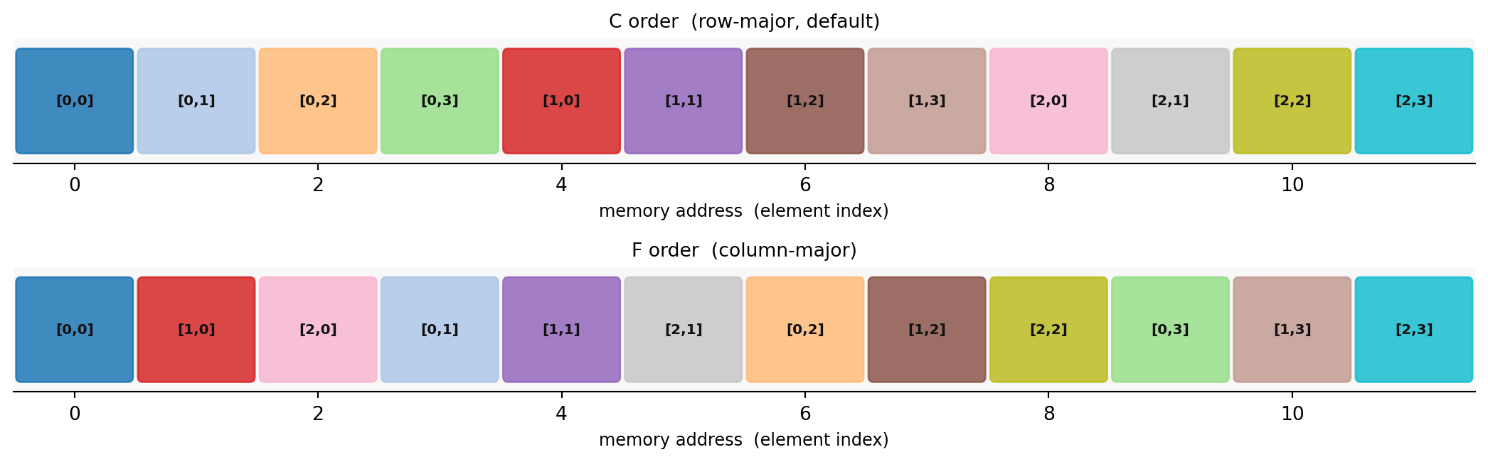
C order (row-major, the default): Elements of the same row are adjacent. Row index changes slowest; column index changes fastest.

F order (column-major): Elements of the same column are adjacent. Column index changes slowest; row index changes fastest.

import numpy as np

A = np.arange(12.0).reshape(3, 4)      # shape (3, 4)  C order (default)
print("C_CONTIGUOUS:", A.flags['C_CONTIGUOUS'])   # True
print("F_CONTIGUOUS:", A.flags['F_CONTIGUOUS'])   # False
print("strides (bytes):", A.strides)               # (32, 8)

B = np.asfortranarray(A)               # shape (3, 4)  F order
print("\nF_CONTIGUOUS:", B.flags['F_CONTIGUOUS'])  # True
print("strides (bytes):", B.strides)               # (8, 24)

C_CONTIGUOUS: True
F_CONTIGUOUS: False
strides (bytes): (32, 8)

F_CONTIGUOUS: True
strides (bytes): (8, 24)

The strides tuple gives the byte step to move one position along each axis. For float64 (8 bytes per element):

C order (3, 4): strides (32, 8) – one row apart = 4 cols * 8 bytes = 32; one col apart = 8 bytes.
F order (3, 4): strides (8, 24) – one row apart = 8 bytes (adjacent); one col apart = 3 rows * 8 bytes = 24.

26.3.2 Visualization

import numpy as np
import matplotlib.pyplot as plt
import matplotlib.patches as mpatches

A = np.arange(12).reshape(3, 4)     # shape (3, 4)
c_order = A.ravel(order='C')        # shape (12,)  row-first sequence
f_order = A.ravel(order='F')        # shape (12,)  column-first sequence

fig, axes = plt.subplots(2, 1, figsize=(11, 3.5))
cmap = plt.get_cmap('tab20')

for ax, label, seq in zip(
    axes,
    ['C order  (row-major, default)', 'F order  (column-major)'],
    [c_order, f_order],
):
    ax.set_xlim(-0.5, 11.5)
    ax.set_ylim(-0.5, 0.5)
    ax.set_yticks([])
    ax.set_title(label, fontsize=10)
    ax.set_xlabel('memory address  (element index)', fontsize=9)
    ax.set_facecolor('#f8f8f8')
    ax.spines[['top', 'right', 'left']].set_visible(False)
    for i, val in enumerate(seq):
        row_idx, col_idx = divmod(int(val), 4)
        color = cmap(val / 12)
        rect = mpatches.FancyBboxPatch(
            (i - 0.44, -0.38), 0.88, 0.76,
            boxstyle='round,pad=0.04', color=color, alpha=0.85,
        )
        ax.add_patch(rect)
        ax.text(i, 0, f'[{row_idx},{col_idx}]', ha='center', va='center',
                fontsize=7.5, fontweight='bold', color='#111111')

plt.tight_layout()
plt.show()

Figure 26.1: A 3x4 matrix stored in memory under C order (row-major, top) and F order (column-major, bottom). Each cell shows the matrix position [row,col]; its horizontal position is its slot in the flat memory buffer.

Same color = same matrix element. In C order, elements [0,0] [0,1] [0,2] [0,3] are the first four memory slots; in F order, [0,0] [1,0] [2,0] are the first three.

26.3.3 Converting Between Orders

import numpy as np

A = np.arange(12.0).reshape(3, 4)     # shape (3, 4)  C order

B = np.asfortranarray(A)              # shape (3, 4)  F order (copies if needed)
C = np.ascontiguousarray(B)           # shape (3, 4)  C order (copies if needed)

print("A: C={}, F={}".format(A.flags['C_CONTIGUOUS'], A.flags['F_CONTIGUOUS']))
print("B: C={}, F={}".format(B.flags['C_CONTIGUOUS'], B.flags['F_CONTIGUOUS']))
print("C: C={}, F={}".format(C.flags['C_CONTIGUOUS'], C.flags['F_CONTIGUOUS']))

A: C=True, F=False
B: C=False, F=True
C: C=True, F=False

Function	Guarantees
`np.ascontiguousarray(A)`	C-contiguous; copies only if not already C
`np.asfortranarray(A)`	F-contiguous; copies only if not already F
`A.copy(order='C')`	C-contiguous copy, always
`A.copy(order='F')`	F-contiguous copy, always

26.3.4 Views, Copies, and Contiguity

Many NumPy operations return views into the same memory buffer. A view may not be contiguous, which matters when passing to C/Fortran libraries.

import numpy as np

A = np.arange(12.0).reshape(3, 4)    # shape (3, 4)  C-contiguous

# Slices are views -- contiguous or not depending on the slice
row = A[0, :]        # shape (4,)   C-contiguous (contiguous row)
col = A[:, 0]        # shape (3,)   NOT contiguous (stride = 32 bytes)

print("row: C_contiguous =", row.flags['C_CONTIGUOUS'])   # True
print("col: C_contiguous =", col.flags['C_CONTIGUOUS'])   # False

# Transpose is a view -- always non-C-contiguous for 2-D matrices
At = A.T             # shape (4, 3)
print("A.T: C_contiguous =", At.flags['C_CONTIGUOUS'])    # False
print("A.T: F_contiguous =", At.flags['F_CONTIGUOUS'])    # True

# reshape returns a view when possible; falls back to copy when not
A_flat = A.ravel()           # shape (12,)  view (C order)
At_flat = A.T.ravel()        # shape (12,)  copy (A.T not C-contiguous)
print("A.ravel() shares memory:", np.shares_memory(A, A_flat))    # True
print("A.T.ravel() shares memory:", np.shares_memory(A, At_flat)) # False

row: C_contiguous = True
col: C_contiguous = False
A.T: C_contiguous = False
A.T: F_contiguous = True
A.ravel() shares memory: True
A.T.ravel() shares memory: False

Rule: If A.flags['C_CONTIGUOUS'] is False, call np.ascontiguousarray(A) before passing to OpenCV, Numba, or any C extension that expects a packed array.

26.3.5 Transpose and Contiguity

Transposing with .T reverses the strides without copying data. The transposed array is F-contiguous (not C-contiguous) for a standard 2-D matrix.

import numpy as np

A  = np.ones((3, 4))     # shape (3, 4)  C-contiguous;  strides (32, 8)
At = A.T                  # shape (4, 3)  view;          strides (8, 32)

print("A  strides:", A.strides,  " C=", A.flags['C_CONTIGUOUS'])
print("At strides:", At.strides, " C=", At.flags['C_CONTIGUOUS'])
print("shares memory:", np.shares_memory(A, At))

# np.linalg handles non-contiguous arrays automatically
vals = np.linalg.eigvalsh(At @ A)    # shape (3,)  -- works fine
print("eigenvalues of A.T @ A:", vals.round(3))

# But cv2.* requires C-contiguous uint8
uint_At = np.ascontiguousarray((At * 100).astype(np.uint8))
print("cv2-safe: C=", uint_At.flags['C_CONTIGUOUS'])

A  strides: (32, 8)  C= True
At strides: (8, 32)  C= False
shares memory: True
eigenvalues of A.T @ A: [-0.  0.  0. 12.]
cv2-safe: C= True

26.3.6 When Layout Matters

Context	Layout requirement	What happens if wrong
`numpy.linalg` / `scipy.linalg`	Either (auto-converted internally)	Silent copy; minor overhead
OpenCV (`cv2.*`)	C-contiguous	May raise or silently corrupt output
Numba JIT (default)	C-contiguous	May fall back to object mode
Row-slicing speed	C order	Rows are contiguous; cache-friendly
Column-slicing speed	F order	Columns are contiguous; cache-friendly
Large BLAS matrix products	Matches BLAS expectations	2-10x slowdown from implicit transpose copies
`scipy.linalg.lapack` direct calls	C or F as documented per routine	Check `overwrite_a` behavior

Practical rule: Create arrays in C order (the default) and call np.ascontiguousarray(A) before passing to OpenCV or Numba.

26.3.7 Performance: Row vs Column Access

Accessing memory in stride order incurs cache misses. For a large C-order matrix, iterating over rows is much faster than iterating over columns.

import numpy as np
import time

n = 2000
A = np.zeros((n, n))    # shape (2000, 2000)  C order

# Row-wise sum: accesses each row contiguously -> fast
t0 = time.perf_counter()
row_sums = A.sum(axis=1)          # shape (2000,)
t_row = time.perf_counter() - t0

# Column-wise sum: accesses memory with stride n*8 bytes -> slower
t0 = time.perf_counter()
col_sums = A.sum(axis=0)          # shape (2000,)
t_col = time.perf_counter() - t0

print(f"row sum time: {t_row*1e3:.2f} ms")
print(f"col sum time: {t_col*1e3:.2f} ms")

row sum time: 7.35 ms
col sum time: 1.48 ms

The difference grows with matrix size. For very large matrices processed column-by-column, consider transposing to F order first.

26.4 Linear Algebra Function Reference

Quick-reference tables for numpy.linalg, scipy.linalg, the sparse submodules, and the supporting SciPy utilities used throughout the book.

26.4.1 `numpy.linalg`

Function	Returns	Notes
`np.linalg.solve(A, b)`	`x`	Square \(Ax = b\); prefer over `inv(A) @ b`
`np.linalg.lstsq(A, b, rcond=None)`	`(x, res, rank, sv)`	Least squares; `rcond=None` silences FutureWarning
`np.linalg.inv(A)`	\(A^{-1}\)	Rarely needed; `solve` is faster and more stable
`np.linalg.pinv(A)`	\(A^+\)	Moore-Penrose pseudoinverse
`np.linalg.det(A)`	scalar	Can overflow; prefer `slogdet` for large matrices
`np.linalg.slogdet(A)`	`(sign, logabsdet)`	Numerically stable log-determinant
`np.linalg.norm(v)`	scalar	2-norm for vectors, Frobenius for matrices
`np.linalg.norm(A, ord=2)`	scalar	Spectral norm (largest singular value)
`np.linalg.norm(A, ord='fro')`	scalar	Frobenius norm
`np.linalg.cond(A)`	scalar	Condition number \(\\|A\\| \cdot \\|A^+\\|\)
`np.linalg.matrix_rank(A)`	int	Rank via SVD
`np.linalg.eig(A)`	`(vals, vecs)`	General matrix; eigenvalues may be complex
`np.linalg.eigh(A)`	`(vals, vecs)`	Symmetric/Hermitian; real, ascending order
`np.linalg.eigvals(A)`	`vals`	Eigenvalues only (no vectors; faster)
`np.linalg.svd(A, full_matrices=False)`	`(U, s, Vt)`	Economy SVD; `s` is 1-D descending
`np.linalg.svd(A, compute_uv=False)`	`s`	Singular values only; returns 1-D array, NOT a tuple
`np.linalg.cholesky(A)`	`L`	Lower Cholesky factor; `A` must be SPD
`np.linalg.qr(A)`	`(Q, R)`	Thin QR by default
`np.linalg.matrix_power(A, n)`	\(A^n\)	Integer powers

import numpy as np

rng = np.random.default_rng(42)
A = rng.standard_normal((4, 4))    # shape (4, 4)
A = A @ A.T + 4.0 * np.eye(4)      # shape (4, 4)  symmetric positive definite
b = rng.standard_normal((4,))      # shape (4,)

x          = np.linalg.solve(A, b)
vals, vecs = np.linalg.eigh(A)                    # vals shape (4,), vecs shape (4, 4)
U, s, Vt   = np.linalg.svd(A, full_matrices=False)  # s shape (4,)  -- 1-D, descending
sv_only    = np.linalg.svd(A, compute_uv=False)   # shape (4,)  -- 1-D array directly
L          = np.linalg.cholesky(A)                # shape (4, 4)

print(f"residual ||Ax-b||     : {np.linalg.norm(A@x - b):.2e}")
print(f"eigenvalues (eigh)    : {vals.round(2)}")
print(f"singular values (svd) : {s.round(2)}")
print(f"Cholesky check ||LLT-A||: {np.linalg.norm(L@L.T - A):.2e}")

residual ||Ax-b||     : 2.29e-16
eigenvalues (eigh)    : [ 4.01  5.05  8.21 11.31]
singular values (svd) : [11.31  8.21  5.05  4.01]
Cholesky check ||LLT-A||: 2.18e-15

26.4.2 `scipy.linalg` (Dense)

Function	Returns	Notes
`scipy.linalg.solve(A, b)`	`x`	Extra: `assume_a='sym'`, `lower`, `transposed`
`scipy.linalg.lu(A)`	`(P, L, U)`	Full LU with partial pivoting
`scipy.linalg.lu_factor(A)`	`(lu, piv)`	Compact packed form
`scipy.linalg.lu_solve((lu, piv), b)`	`x`	Solve with pre-factored matrix; efficient for many RHS
`scipy.linalg.cho_factor(A)`	`(c, lower)`	Cholesky; `A` must be SPD
`scipy.linalg.cho_solve((c, lower), b)`	`x`	Solve with pre-factored Cholesky
`scipy.linalg.svd(A, full_matrices=False)`	`(U, s, Vt)`	Adds `lapack_driver` option
`scipy.linalg.svd(A, ..., lapack_driver='gesdd')`	`(U, s, Vt)`	Divide-and-conquer; fastest for large dense
`scipy.linalg.eigh(A)`	`(vals, vecs)`	Symmetric; ascending eigenvalues
`scipy.linalg.eigh(A, B)`	`(vals, vecs)`	Generalized problem \(Ax = \lambda Bx\)
`scipy.linalg.expm(A)`	\(e^A\)	Matrix exponential; use for Lie group exp maps
`scipy.linalg.logm(A)`	\(\log A\)	Matrix logarithm

import numpy as np
import scipy.linalg

rng = np.random.default_rng(0)
A = rng.standard_normal((4, 4))    # shape (4, 4)
A = A @ A.T + 4.0 * np.eye(4)      # shape (4, 4)  SPD
B = rng.standard_normal((4, 3))    # shape (4, 3)  multiple right-hand sides

# Pre-factor once, solve multiple right-hand sides cheaply
lu, piv = scipy.linalg.lu_factor(A)                 # packed factorization
X       = scipy.linalg.lu_solve((lu, piv), B)        # shape (4, 3)
print(f"LU solve ||AX-B||      : {np.linalg.norm(A @ X - B):.2e}")

# Cholesky
c, lower = scipy.linalg.cho_factor(A)                # packed Cholesky
x_cho    = scipy.linalg.cho_solve((c, lower), B[:, 0])  # shape (4,)
print(f"Cholesky solve ||Ax-b||: {np.linalg.norm(A @ x_cho - B[:, 0]):.2e}")

# Matrix exponential: skew-symmetric -> rotation
W = np.array([[0., -1.], [1., 0.]])    # shape (2, 2)  90-degree generator
expW = scipy.linalg.expm(W)            # shape (2, 2)  rotation matrix
print(f"expm([[0,-1],[1,0]]) =\n{expW.round(4)}")

LU solve ||AX-B||      : 3.74e-16
Cholesky solve ||Ax-b||: 1.31e-16
expm([[0,-1],[1,0]]) =
[[ 0.5403 -0.8415]
 [ 0.8415  0.5403]]

26.4.3 `scipy.sparse` Formats

Class / Constructor	Format	When to use
`scipy.sparse.csr_matrix(A)`	Compressed Sparse Row	Row slicing, matrix-vector products
`scipy.sparse.csc_matrix(A)`	Compressed Sparse Column	Column slicing, sparse direct solvers
`scipy.sparse.coo_matrix((data, (rows, cols)), shape)`	Coordinate (triplet)	Incremental construction
`scipy.sparse.diags(diagonals, offsets, shape)`	Diagonal / banded	Tridiagonal and similar
`scipy.sparse.eye(n, format='csr')`	Sparse identity
`scipy.sparse.bmat([[A, B], [C, D]])`	Block	Block-structured systems

26.4.4 `scipy.sparse.linalg` Solvers

Function	Use for	Notes
`spsolve(A, b)`	Direct sparse solve	SuperLU; single RHS
`factorized(A)`	Reuse LU across RHS	Returns callable `solve_fn(b)`
`splu(A)`	Sparse LU object	`.solve(b)` for each RHS
`cg(A, b)`	SPD iterative solve	Conjugate Gradient; `M` for preconditioner
`gmres(A, b)`	General iterative solve	Restarts Krylov
`lsqr(A, b)`	Sparse least squares	Returns `(x, flag, rnorm, ...)`
`eigsh(A, k)`	Top-\(k\) eigenvalues, symmetric	Lanczos / ARPACK
`svds(A, k)`	Top-\(k\) singular triplets	Returns ascending order (opposite of `np.linalg.svd`)

import numpy as np
import scipy.sparse
import scipy.sparse.linalg

n = 100
# Tridiagonal matrix (typical in finite differences)
A_sp = scipy.sparse.diags(
    [4.0 * np.ones(n), -np.ones(n - 1), -np.ones(n - 1)],
    offsets=[0, 1, -1],
    format='csr',
)   # shape (100, 100)

rng = np.random.default_rng(0)
b   = rng.standard_normal((n,))    # shape (100,)

x = scipy.sparse.linalg.spsolve(A_sp, b)        # shape (100,)
print(f"spsolve residual : {np.linalg.norm(A_sp @ x - b):.2e}")

# Top-3 eigenvalues (ascending order from eigsh)
vals, vecs = scipy.sparse.linalg.eigsh(A_sp, k=3, which='SM')
print(f"3 smallest eigenvalues: {vals.round(3)}")

spsolve residual : 1.35e-15
3 smallest eigenvalues: [2.001 2.004 2.009]

26.4.5 `scipy.spatial.transform.Rotation`

Rotation objects represent SO(3) rotations and convert between representations. The quaternion convention is scalar-last [x, y, z, w].

Method	Description
`Rotation.from_matrix(R)`	From `(3, 3)` rotation matrix
`Rotation.from_rotvec(v)`	Axis-angle; angle \(= \\|v\\|\) in radians
`Rotation.from_euler('xyz', angles)`	Extrinsic Euler angles; `degrees=True` available
`Rotation.from_quat([x, y, z, w])`	Quaternion, scalar-last convention
`.as_matrix()`	To `(3, 3)` array
`.as_rotvec()`	To axis-angle vector
`.as_euler('xyz')`	To Euler angles
`.as_quat()`	To `[x, y, z, w]`
`r1 * r2`	Compose (\(R_1 R_2\))
`r.inv()`	Inverse (\(R^T\))
`r.apply(v)`	Rotate; `v` shape `(3,)` or `(n, 3)`

import numpy as np
from scipy.spatial.transform import Rotation

# 90-degree rotation about the z-axis
r  = Rotation.from_euler('z', 90, degrees=True)
R  = r.as_matrix()    # shape (3, 3)
q  = r.as_quat()      # shape (4,)  [x, y, z, w]

print("R:\n", R.round(4))
print("q:", q.round(4))

# Rotate a vector
v = np.array([1.0, 0.0, 0.0])                 # shape (3,)
print("r.apply([1,0,0]) :", r.apply(v).round(4))   # [0, 1, 0]

# Composition and inverse
r2  = Rotation.from_euler('z', -90, degrees=True)
r12 = r * r2    # should be near identity
print("r * r.inv() max error:", (r12.as_matrix() - np.eye(3)).max())

R:
 [[ 0. -1.  0.]
 [ 1.  0.  0.]
 [ 0.  0.  1.]]
q: [0.     0.     0.7071 0.7071]
r.apply([1,0,0]) : [0. 1. 0.]
r * r.inv() max error: 0.0

26.4.6 `scipy.ndimage.affine_transform`

Applies an affine transformation in image (row-column) coordinates. Internally it computes the inverse map: for each output pixel it finds the corresponding input location and interpolates.

Parameter	Meaning
`input`	Input image `(H, W)` or `(H, W, C)`
`matrix`	`(2, 2)` linear part of the inverse transform
`offset`	Translation of the inverse transform
`order`	Interpolation order: 0 = nearest, 1 = bilinear, 3 = cubic
`cval`	Fill value for out-of-bounds pixels

Pass the matrix for \(-\theta\) to rotate the image by \(+\theta\).

import numpy as np
import scipy.ndimage
import matplotlib.pyplot as plt

# Synthetic grayscale image: bright rectangle on dark background
img = np.zeros((80, 80), dtype=np.float64)    # shape (80, 80)
img[20:60, 20:60] = 1.0

# Rotate by +30 degrees: pass the inverse rotation (−30 deg)
theta = np.radians(-30.0)
c, s  = np.cos(theta), np.sin(theta)
R_inv = np.array([[c, -s], [s, c]])            # shape (2, 2)  inverse map

# Offset so rotation is about the image center
cx, cy = 40.0, 40.0
offset = np.array([cx, cy]) - R_inv @ np.array([cx, cy])  # shape (2,)

rotated = scipy.ndimage.affine_transform(
    img, R_inv, offset=offset, order=1, cval=0.0,
)   # shape (80, 80)

fig, axes = plt.subplots(1, 2, figsize=(6, 3))
for ax, im, title in zip(axes, [img, rotated], ['Original', 'Rotated +30 deg']):
    ax.imshow(im, cmap='gray', vmin=0, vmax=1)
    ax.set_title(title, fontsize=9)
    ax.axis('off')
plt.tight_layout()
plt.show()

26.4.7 `scipy.stats.chi2`

Used in Chapters 19-23 for Mahalanobis thresholds and Gaussian confidence ellipsoids.

Call	Description
`chi2.ppf(p, df=k)`	\(p\)-th quantile: the threshold \(c\) such that \(P(X \le c) = p\)
`chi2.cdf(x, df=k)`	Cumulative probability \(P(X \le x)\)
`chi2.sf(x, df=k)`	Survival function \(P(X > x) = 1 - \text{CDF}\)

from scipy.stats import chi2

# 95% confidence region for a 2-D Gaussian (Mahalanobis distance threshold)
df = 2
threshold = chi2.ppf(0.95, df=df)
prob_outside = chi2.sf(threshold, df=df)

print(f"chi2(df={df}).ppf(0.95)       = {threshold:.4f}")
print(f"P(chi2({df}) > {threshold:.4f}) = {prob_outside:.4f}")

chi2(df=2).ppf(0.95)       = 5.9915
P(chi2(2) > 5.9915) = 0.0500

26.4.8 Decision Guide

Situation	Recommended function
Square linear system, single solve	`np.linalg.solve`
Square system, same matrix, many RHS	`scipy.linalg.lu_factor` + `lu_solve`
Symmetric positive definite system	`scipy.linalg.cho_factor` + `cho_solve`
Overdetermined / least squares	`np.linalg.lstsq`
Large sparse system (direct)	`scipy.sparse.linalg.spsolve`
Large sparse SPD (iterative)	`scipy.sparse.linalg.cg`
All eigenvalues, symmetric dense	`np.linalg.eigh` or `scipy.linalg.eigh`
Top-\(k\) eigenvalues, large sparse	`scipy.sparse.linalg.eigsh`
All singular values, dense	`np.linalg.svd`
Top-\(k\) singular values, large	`scipy.sparse.linalg.svds`
Matrix exponential / logarithm	`scipy.linalg.expm` / `logm`
SO(3) rotation conversions	`scipy.spatial.transform.Rotation`
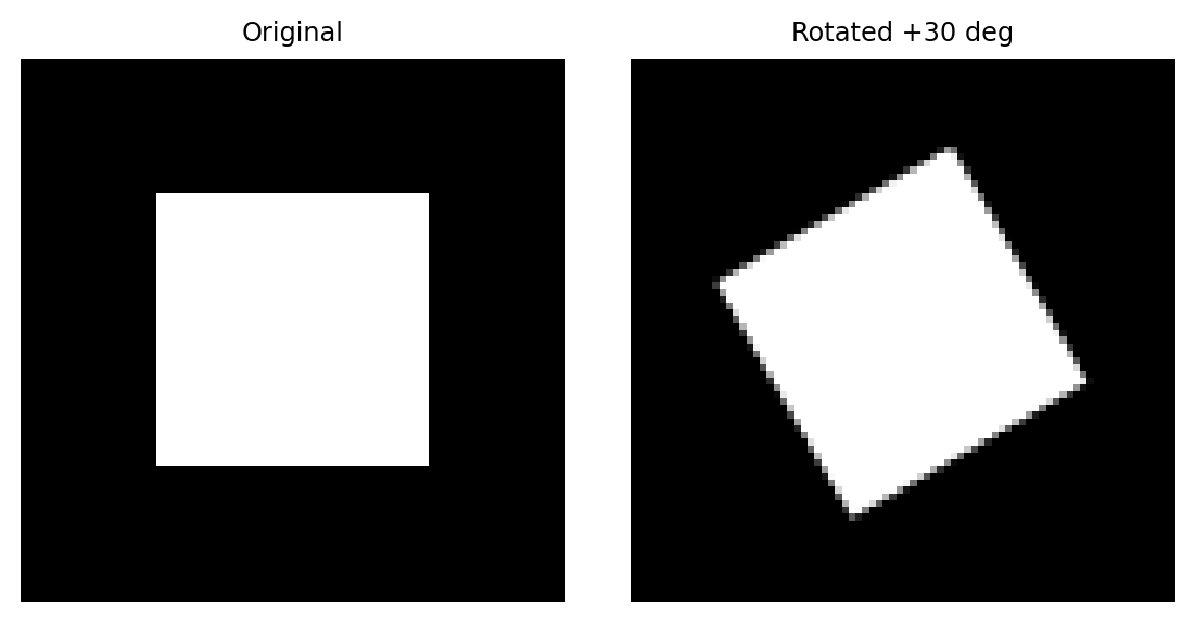
2-D / 3-D image affine warp	`scipy.ndimage.affine_transform`
Chi-squared confidence thresholds	`scipy.stats.chi2.ppf`

26.5 OpenCV Quick Reference

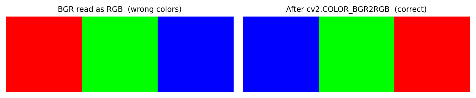
OpenCV differs from NumPy/matplotlib in two critical ways: channel order is BGR not RGB, and the default image dtype is uint8 in [0, 255].

26.5.1 Image Format Conventions

Property	matplotlib / PIL	OpenCV
Color channel order	RGB	BGR
Color image shape	`(H, W, 3)`	`(H, W, 3)`
Grayscale image shape	`(H, W)`	`(H, W)` (no channel axis)
Default dtype	float64 or uint8	uint8 [0, 255]
Size argument order	`(H, W)`	`(W, H)` i.e. `(width, height)`

cv2.resize(img, (W, H)) takes width-first. img.shape[:2] returns (H, W) height-first. These are the opposite of each other.

26.5.2 I/O Functions

Function	Description
`cv2.imread(path)`	Load image; returns `(H, W, 3)` BGR uint8, or `None` on failure
`cv2.imread(path, cv2.IMREAD_GRAYSCALE)`	Load as `(H, W)` grayscale
`cv2.imread(path, cv2.IMREAD_UNCHANGED)`	Preserve alpha channel
`cv2.imwrite(path, img)`	Save; format inferred from file extension

import cv2

img = cv2.imread('photo.jpg')          # shape (H, W, 3)  uint8  BGR
if img is None:
    raise FileNotFoundError('cv2.imread returned None -- check the path')

print(img.shape, img.dtype)            # e.g. (480, 640, 3) uint8
cv2.imwrite('output.png', img)

26.5.3 Color Conversion

import numpy as np
import cv2
import matplotlib.pyplot as plt

# Synthetic BGR image: three solid patches
img_bgr = np.zeros((80, 240, 3), dtype=np.uint8)    # shape (80, 240, 3)
img_bgr[:, :80,   0] = 255   # pure blue in BGR  (B=255, G=0, R=0)
img_bgr[:, 80:160, 1] = 255  # pure green in BGR (B=0, G=255, R=0)
img_bgr[:, 160:,   2] = 255  # pure red in BGR   (B=0, G=0, R=255)

img_rgb = cv2.cvtColor(img_bgr, cv2.COLOR_BGR2RGB)   # shape (80, 240, 3)  RGB

fig, axes = plt.subplots(1, 2, figsize=(8, 2.2))
axes[0].imshow(img_bgr)
axes[0].set_title('BGR read as RGB  (wrong colors)', fontsize=9)
axes[0].axis('off')
axes[1].imshow(img_rgb)
axes[1].set_title('After cv2.COLOR_BGR2RGB  (correct)', fontsize=9)
axes[1].axis('off')
plt.tight_layout()
plt.show()

Figure 26.2: A synthetic test image displayed without and with BGR-to-RGB conversion. OpenCV’s pure-blue patch [255,0,0] in BGR appears red when matplotlib reads it as RGB (left). After cv2.cvtColor(img, cv2.COLOR_BGR2RGB) the colors are correct (right).

Conversion code	Description
`cv2.COLOR_BGR2RGB`	BGR to RGB – required before `plt.imshow`
`cv2.COLOR_BGR2GRAY`	BGR to grayscale `(H, W)`
`cv2.COLOR_GRAY2BGR`	Grayscale to 3-channel BGR
`cv2.COLOR_BGR2HSV`	BGR to Hue-Saturation-Value
`cv2.COLOR_BGR2LAB`	BGR to CIELAB perceptual space
`cv2.COLOR_RGB2BGR`	RGB (from matplotlib/PIL) to BGR

26.5.4 Geometric Transforms

Function	Description
`cv2.getPerspectiveTransform(src4, dst4)`	Homography from 4 point pairs; returns `(3, 3)`
`cv2.findHomography(src_pts, dst_pts)`	Robust homography from many points (RANSAC)
`cv2.warpPerspective(img, M, (W, H))`	Apply `(3, 3)` homography
`cv2.getRotationMatrix2D(center, angle_deg, scale)`	Returns `(2, 3)` affine matrix
`cv2.warpAffine(img, M23, (W, H))`	Apply `(2, 3)` affine matrix
`cv2.resize(img, (W, H))`	Resize image; size argument is `(width, height)`
`cv2.flip(img, 1)`	Flip: 0 = vertical, 1 = horizontal, -1 = both

import numpy as np
import cv2

# Synthetic image with a white rectangle
src_img = np.zeros((200, 200, 3), dtype=np.uint8)    # shape (200, 200, 3)
cv2.rectangle(src_img, (40, 40), (160, 160), (200, 200, 200), -1)

# Four corresponding points (float32 required)
src_pts = np.float32([[40, 40], [160, 40], [160, 160], [40, 160]])
dst_pts = np.float32([[ 0,  0], [200,  0], [180, 200], [20,  200]])

M   = cv2.getPerspectiveTransform(src_pts, dst_pts)  # shape (3, 3)
dst = cv2.warpPerspective(src_img, M, (200, 200))    # shape (200, 200, 3)
print("M:\n", M.round(3))
print("output shape:", dst.shape, dst.dtype)

M:
 [[  1.818   0.227 -81.818]
 [ -0.      2.273 -90.909]
 [  0.      0.002   1.   ]]
output shape: (200, 200, 3) uint8

26.5.5 Camera Calibration Pipeline

import cv2
import numpy as np

# Object points: corners on a flat chessboard (Z=0)
pattern = (9, 6)    # inner corners per row, column
objp = np.zeros((pattern[0] * pattern[1], 3), dtype=np.float32)   # shape (54, 3)
objp[:, :2] = np.mgrid[0:pattern[0], 0:pattern[1]].T.reshape(-1, 2)

obj_pts, img_pts = [], []
for fname in image_files:
    img  = cv2.imread(fname)
    gray = cv2.cvtColor(img, cv2.COLOR_BGR2GRAY)
    ret, corners = cv2.findChessboardCorners(gray, pattern)
    if ret:
        corners = cv2.cornerSubPix(
            gray, corners, (11, 11), (-1, -1),
            (cv2.TERM_CRITERIA_EPS + cv2.TERM_CRITERIA_MAX_ITER, 30, 0.001),
        )
        obj_pts.append(objp)
        img_pts.append(corners)

ret, K, dist, rvecs, tvecs = cv2.calibrateCamera(
    obj_pts, img_pts, gray.shape[::-1], None, None,
)
# K    : shape (3, 3)  intrinsic matrix
# dist : shape (1, 5)  [k1, k2, p1, p2, k3]
undistorted = cv2.undistort(img, K, dist)

26.5.6 Stereo Pipeline Summary

Step	Function
Compute rectification transforms	`cv2.stereoRectify(K1, d1, K2, d2, size, R, t)`
Precompute remap lookup tables	`cv2.initUndistortRectifyMap(K, dist, R, P, size, cv2.CV_32FC1)`
Apply rectification to images	`cv2.remap(img, map_x, map_y, cv2.INTER_LINEAR)`
Compute disparity map	`stereo = cv2.StereoSGBM_create(...); disp = stereo.compute(l, r)`
Convert disparity to 3-D	`depth = cv2.reprojectImageTo3D(disp / 16.0, Q)`

StereoSGBM.compute returns int16 with disparity multiplied by 16. Divide by 16.0 before passing to reprojectImageTo3D. depth has shape (H, W, 3) – the last axis is (X, Y, Z) in camera frame.

26.5.7 Common Pitfalls

Pitfall	Symptom	Fix
BGR vs RGB	Wrong colors in `plt.imshow`	`cv2.cvtColor(img, cv2.COLOR_BGR2RGB)`
`imread` returns `None`	Crash on `None.shape`	Always check `if img is None:` after loading
Size is `(W, H)` not `(H, W)`	Stretched or transposed output	Remember: `img.shape = (H, W, C)` but `cv2.resize(img, (W, H))`
`uint8` arithmetic overflow	Clipping / wrapping artifacts	Cast to `float32` first; clamp and cast back to `uint8`
Not C-contiguous array	`cv2` error or silent failure	`np.ascontiguousarray(A)` before passing to `cv2`
Float image outside [0, 255]	Black output in `imwrite`	Multiply float by 255; cast to `uint8`
Disparity not divided by 16	Depth map is 16x too far	`disp.astype(np.float32) / 16.0` before `reprojectImageTo3D`