10  Camera Models and Projection Matrices

10.1 Pinhole Camera Geometry

Every photograph collapses a 3D scene onto a 2D sensor. Understanding how that collapse works — mathematically — is the foundation for 3D reconstruction, AR overlays, robot navigation, and autonomous vehicles. The simplest model that captures all the essential geometry is the pinhole camera.

---

10.1.1 The Physical Idea

Imagine a box with a tiny hole on one face and a film plane on the opposite face. Light from a scene point \(\mathbf{P}\) travels through the hole (the optical centre \(\mathbf{O}\)) and lands at image point \(\mathbf{p}\).

The key parameters: - Focal length \(f\): distance from optical centre to image plane (mm or pixels). - Image plane: the sensor, at distance \(f\) behind \(\mathbf{O}\). - Optical axis: the \(z\)-axis of the camera frame, pointing forward.

---

10.1.2 Deriving the Projection Equations

Place the optical centre at the origin. A scene point at camera coordinates \((X, Y, Z)\) projects to image coordinates \((x, y)\) by similar triangles:

\[\frac{x}{f} = \frac{X}{Z} \implies x = f \frac{X}{Z}\] \[\frac{y}{f} = \frac{Y}{Z} \implies y = f \frac{Y}{Z}\]

This is perspective projection (also called central projection). The depth \(Z\) appears in the denominator — objects farther away look smaller.

import numpy as np
import matplotlib.pyplot as plt

def project_pinhole(P, f=1.0):
    """Project 3D camera-frame points P (shape N×3) with focal length f.
    Returns image points shape (N, 2)."""
    X, Y, Z = P[:, 0], P[:, 1], P[:, 2]   # each shape (N,)
    x = f * X / Z                           # shape (N,)
    y = f * Y / Z                           # shape (N,)
    return np.column_stack([x, y])          # shape (N, 2)

# A unit cube at Z = 3 m (camera space)
corners_3d = np.array([
    [-0.5, -0.5, 3.0],
    [ 0.5, -0.5, 3.0],
    [ 0.5,  0.5, 3.0],
    [-0.5,  0.5, 3.0],
    [-0.5, -0.5, 3.0],  # close the loop
])   # shape (5, 3)

# Same cube at Z = 6 m (twice as far)
corners_far = corners_3d.copy()
corners_far[:, 2] = 6.0   # shape (5, 3)

proj_near = project_pinhole(corners_3d, f=2.0)   # shape (5, 2)
proj_far  = project_pinhole(corners_far, f=2.0)  # shape (5, 2)

fig, ax = plt.subplots(figsize=(5, 5))
ax.plot(proj_near[:, 0], proj_near[:, 1], color='#4a90d9', lw=2.5, label='Z = 3 m')
ax.plot(proj_far[:,  0], proj_far[:,  1], color='tomato',  lw=2.5, label='Z = 6 m', ls='--')
ax.set_aspect('equal')
ax.set_xlabel('x (image, m)'); ax.set_ylabel('y (image, m)')
ax.set_title('Pinhole Projection: Farther Objects Look Smaller', fontsize=11)
ax.legend(); ax.grid(True, alpha=0.2)
ax.axhline(0, color='#333333', lw=0.4, alpha=0.5)
ax.axvline(0, color='#333333', lw=0.4, alpha=0.5)
plt.tight_layout()
plt.show()

---

10.1.3 Homogeneous Form

The division by \(Z\) makes projection nonlinear — inconvenient for algebra. Homogeneous coordinates fix that. In homogeneous form, a 2D image point \((x, y)\) is represented as any scalar multiple of \([x, y, 1]^T\), and the projection becomes a linear matrix multiplication:

\[\lambda \begin{pmatrix}x\\y\\1\end{pmatrix} = \begin{pmatrix}f & 0 & 0 & 0\\ 0 & f & 0 & 0\\ 0 & 0 & 1 & 0\end{pmatrix} \begin{pmatrix}X\\Y\\Z\\1\end{pmatrix}\]

where \(\lambda = Z\) is the depth (the scale factor that gets divided out).

import numpy as np

f = 2.0

# Simplified projection matrix (metric image plane, centre at origin)
P_simple = np.array([
    [f, 0., 0., 0.],
    [0., f, 0., 0.],
    [0., 0., 1., 0.],
])   # shape (3, 4)

P_world = np.array([1.5, -0.5, 4.0, 1.0])   # shape (4,) — homogeneous 3D point

p_h = P_simple @ P_world   # shape (3,) — homogeneous image point
x, y = p_h[0] / p_h[2], p_h[1] / p_h[2]   # divide by lambda=Z

print(f"3D point (camera frame): X={P_world[0]}, Y={P_world[1]}, Z={P_world[2]}")
print(f"Projected (homogeneous): {p_h}")
print(f"Image coordinates:       x={x:.4f}, y={y:.4f}")

# Verify against direct formula
print(f"\nDirect f*X/Z = {f*P_world[0]/P_world[2]:.4f}  ✓")
print(f"Direct f*Y/Z = {f*P_world[1]/P_world[2]:.4f}  ✓")

3D point (camera frame): X=1.5, Y=-0.5, Z=4.0
Projected (homogeneous): [ 3. -1.  4.]
Image coordinates:       x=0.7500, y=-0.2500

Direct f*X/Z = 0.7500  ✓
Direct f*Y/Z = -0.2500  ✓

---

10.1.4 Why Depth Information Is Lost

Projection is a many-to-one map: every point along a ray through \(\mathbf{O}\) maps to the same image point. This is why a single image cannot recover depth — you need either stereo, structure from motion, or a depth sensor.

import numpy as np
import matplotlib.pyplot as plt

f = 1.5

# All these 3D points map to the same image point
Z_vals = np.array([1., 2., 4., 8.])   # shape (4,)
target_x, target_y = 0.5, 0.3         # fixed image point

# Back-project: 3D ray at each depth
X_vals = target_x / f * Z_vals   # shape (4,)
Y_vals = target_y / f * Z_vals   # shape (4,)

fig = plt.figure(figsize=(8, 4))
ax = fig.add_subplot(111, projection='3d')

# Draw the projection ray
Z_ray = np.linspace(0.5, 9, 50)
X_ray = target_x / f * Z_ray
Y_ray = target_y / f * Z_ray
ax.plot(Z_ray, X_ray, Y_ray, color='#333333', lw=1, alpha=0.4, ls='--')

# Points along the ray
ax.scatter(Z_vals, X_vals, Y_vals, c=['#4a90d9','#2ecc71','tomato','#f39c12'],
           s=80, zorder=5)

ax.scatter([0], [0], [0], c='black', s=100, marker='^', label='Optical centre')
ax.set_xlabel('Z (depth, m)'); ax.set_ylabel('X'); ax.set_zlabel('Y')
ax.set_title('All points on this ray → same image pixel', fontsize=10)
ax.view_init(elev=15, azim=-75)
plt.tight_layout()
plt.show()

10.2 Intrinsic Matrix \(K\)

The simple pinhole model from §10.1 assumed the image origin is at the optical axis and that pixels are square. Real sensors have a principal point offset, possibly non-square pixels, and occasionally a skew term. All of this is packed into the intrinsic matrix \(K\) — a 3×3 upper-triangular matrix that maps metric camera-frame rays to pixel coordinates.

\[K = \begin{pmatrix} f_x & s & c_x \\ 0 & f_y & c_y \\ 0 & 0 & 1 \end{pmatrix}\]

---

10.2.1 What Each Entry Means

Parameter	Meaning	Typical value (RealSense D435, 640×480)
\(f_x\)	Focal length in pixels along \(x\)	~615 px
\(f_y\)	Focal length in pixels along \(y\)	~615 px
\(s\)	Skew (non-rectangular pixels)	≈ 0 for modern sensors
\(c_x\)	Principal point \(x\) (where optical axis hits sensor)	~320 px
\(c_y\)	Principal point \(y\)	~240 px

Focal length in pixels = focal length in metres × sensor pixels per metre. A 4 mm lens on a sensor with 1500 px/mm gives \(f_x \approx 6000\) px.

---

10.2.2 Applying K: Metric Image → Pixel

Given a camera-frame ray direction \((X/Z, Y/Z)\), \(K\) converts to pixel coordinates \((u, v)\):

\[\begin{pmatrix}u\\v\\1\end{pmatrix} \sim K \begin{pmatrix}X/Z\\Y/Z\\1\end{pmatrix} = \begin{pmatrix}f_x X/Z + s Y/Z + c_x \\ f_y Y/Z + c_y \\ 1\end{pmatrix}\]

import numpy as np

K = np.array([
    [615.,   0., 320.],
    [  0., 615., 240.],
    [  0.,   0.,   1.],
])   # shape (3, 3) — RealSense D435i approximate intrinsics

# A scene point at camera coordinates (0.3, -0.2, 1.5 m)
P_C = np.array([0.3, -0.2, 1.5])   # shape (3,)

# Project: K @ (P_C / P_C[2]) — divide by Z first to normalise
p_norm = P_C / P_C[2]              # shape (3,) — normalised camera ray [X/Z, Y/Z, 1]
p_h    = K @ p_norm                # shape (3,) — homogeneous pixel
u, v   = p_h[0], p_h[1]           # already divided since p_norm[2]=1

print(f"Camera-frame point: {P_C}")
print(f"Normalised ray:     {p_norm.round(6)}")
print(f"Pixel coordinates:  u={u:.2f}, v={v:.2f}")

Camera-frame point: [ 0.3 -0.2  1.5]
Normalised ray:     [ 0.2      -0.133333  1.      ]
Pixel coordinates:  u=443.00, v=158.00

---

10.2.3 Inverting K: Pixel → Camera-Frame Ray

Given a pixel \((u, v)\), \(K^{-1}\) recovers the normalised camera-frame direction — the back-projection ray. This is exactly what the RealSense SDK does when it lifts depth pixels to 3D (§9.7).

For upper-triangular \(K\), the inverse is cheap and exact:

import numpy as np

K = np.array([
    [615.,   0., 320.],
    [  0., 615., 240.],
    [  0.,   0.,   1.],
])   # shape (3, 3)

K_inv = np.linalg.inv(K)   # shape (3, 3)
print("K_inv:")
print(K_inv.round(8))

# Pixel (400, 200) — back-project to unit ray
pixel_h = np.array([400., 200., 1.])   # shape (3,)
ray = K_inv @ pixel_h                  # shape (3,)
print(f"\nPixel (400, 200) → ray: {ray.round(6)}")
print(f"Normalised:             {(ray/ray[2]).round(6)}")

K_inv:
[[ 0.00162602  0.         -0.5203252 ]
 [ 0.          0.00162602 -0.3902439 ]
 [ 0.          0.          1.        ]]

Pixel (400, 200) → ray: [ 0.130081 -0.065041  1.      ]
Normalised:             [ 0.130081 -0.065041  1.      ]

---

10.2.4 Visualising the Principal Point

The principal point \((c_x, c_y)\) is where the optical axis pierces the image sensor. It’s not necessarily at the pixel-coordinate origin — it’s typically near but not exactly at the image centre.

import numpy as np
import matplotlib.pyplot as plt

# Simulate two cameras with different principal points
Ks = {
    'Ideal (cx=320, cy=240)':   np.array([[615.,0.,320.],[0.,615.,240.],[0.,0.,1.]]),
    'Offset (cx=300, cy=255)':  np.array([[615.,0.,300.],[0.,615.,255.],[0.,0.,1.]]),
}

# Project a horizontal bar of points at Z=2 m
Xs = np.linspace(-0.5, 0.5, 9)
Ys = np.zeros(9)
Zs = np.full(9, 2.)
pts_C = np.column_stack([Xs, Ys, Zs])   # shape (9, 3)

fig, ax = plt.subplots(figsize=(7, 4))
colors = ['#4a90d9', 'tomato']
for (label, K), col in zip(Ks.items(), colors):
    uvs = []
    for P in pts_C:
        p_h = K @ (P / P[2])
        uvs.append(p_h[:2])
    uvs = np.array(uvs)   # shape (9, 2)
    ax.plot(uvs[:, 0], uvs[:, 1], 'o-', color=col, lw=2, label=label)
    # Mark principal point
    ax.scatter([K[0,2]], [K[1,2]], marker='+', s=200, color=col, linewidths=2)

ax.set_xlabel('u (px)'); ax.set_ylabel('v (px)')
ax.set_title('Effect of Principal Point Offset on Projected Positions', fontsize=10)
ax.legend(fontsize=9)
ax.grid(True, alpha=0.2)
ax.axhline(240, color='#333333', lw=0.4, alpha=0.5)
ax.axvline(320, color='#333333', lw=0.4, alpha=0.5)
plt.tight_layout()
plt.show()

---

10.2.5 Skew

The skew term \(s\) is nonzero when the pixel axes are not perpendicular. This almost never happens with modern CMOS sensors (\(s \approx 0\)), but it can arise in scanned film or older CCD arrays.

import numpy as np
import matplotlib.pyplot as plt

# Compare s=0 vs s=30 (exaggerated)
K_noskew = np.array([[500., 0.,  320.],[0., 500., 240.],[0.,0.,1.]])
K_skew   = np.array([[500.,30.,  320.],[0., 500., 240.],[0.,0.,1.]])

# Project a square grid of points
grid = []
for x in np.linspace(-0.3, 0.3, 5):
    for y in np.linspace(-0.3, 0.3, 5):
        grid.append([x, y, 1.5])
grid = np.array(grid)   # shape (25, 3)

def project(pts, K):
    return np.array([K @ (p/p[2]) for p in pts])[:, :2]   # shape (N, 2)

fig, axes = plt.subplots(1, 2, figsize=(9, 4))
for ax, K, title, col in [
    (axes[0], K_noskew, 'No skew (s = 0)',  '#4a90d9'),
    (axes[1], K_skew,   'With skew (s = 30)', 'tomato')]:
    pts = project(grid, K)
    ax.scatter(pts[:, 0], pts[:, 1], color=col, s=40)
    ax.set_title(title, fontsize=10)
    ax.set_xlabel('u (px)'); ax.set_ylabel('v (px)')
    ax.set_aspect('equal'); ax.grid(True, alpha=0.2)
    ax.axhline(240, color='#333333', lw=0.4, alpha=0.5)
    ax.axvline(320, color='#333333', lw=0.4, alpha=0.5)

fig.suptitle('Pixel skew shears the projected grid', fontsize=11)
plt.tight_layout()
plt.show()

10.3 Extrinsic Matrix and Full Projection \(P = K[R \mid \mathbf{t}]\)

The intrinsic matrix \(K\) (§10.2) works in camera coordinates. The extrinsic matrix \([R \mid \mathbf{t}]\) maps a 3D world point to camera coordinates first. Together they form the full projection matrix:

\[P = K [R \mid \mathbf{t}] \in \mathbb{R}^{3 \times 4}\]

\[\lambda \begin{pmatrix}u\\v\\1\end{pmatrix} = K \begin{bmatrix}R & \mathbf{t}\end{bmatrix} \begin{pmatrix}X_w\\Y_w\\Z_w\\1\end{pmatrix}\]

where \((X_w, Y_w, Z_w)\) is a world-frame 3D point and \((u, v)\) is its pixel-coordinate image.

---

10.3.1 What \([R \mid \mathbf{t}]\) Means

\([R \mid \mathbf{t}]\) is the first three rows of the 4×4 SE(3) matrix \(T_{\text{camera}\leftarrow\text{world}}\):

• \(R\) — the camera’s orientation relative to the world (3×3)
• \(\mathbf{t}\) — the world origin expressed in camera coordinates (not the camera position in the world!)

Common confusion: The camera position in world coordinates is \(\mathbf{C} = -R^T \mathbf{t}\).

import numpy as np

def Rz(g):
    c, s = np.cos(g), np.sin(g)
    return np.array([[c,-s,0.],[s,c,0.],[0.,0.,1.]])

# Camera is at world position (3, 0, 0), rotated 90° about z
# → in camera frame, world origin is at (-R @ t_world)
cam_pos_world = np.array([3., 0., 0.])   # shape (3,) — camera position in world
R = Rz(np.pi / 2)                        # shape (3, 3)

# t = -R @ cam_pos_world  (standard convention)
t = -R @ cam_pos_world                   # shape (3,)

print(f"Camera position in world:  {cam_pos_world}")
print(f"R (camera orientation):    \n{R.round(4)}")
print(f"t (extrinsic translation): {t.round(4)}")

# Verify: camera centre C = -R^T t = cam_pos_world
C = -R.T @ t
print(f"\nRecovered camera centre:   {C.round(6)}")
print(f"Matches cam_pos_world?     {np.allclose(C, cam_pos_world)}")

Camera position in world:  [3. 0. 0.]
R (camera orientation):    
[[ 0. -1.  0.]
 [ 1.  0.  0.]
 [ 0.  0.  1.]]
t (extrinsic translation): [-0. -3.  0.]

Recovered camera centre:   [3. 0. 0.]
Matches cam_pos_world?     True

---

10.3.2 Full Projection Matrix

import numpy as np

def Rz(g):
    c, s = np.cos(g), np.sin(g)
    return np.array([[c,-s,0.],[s,c,0.],[0.,0.,1.]])

K = np.array([
    [615.,   0., 320.],
    [  0., 615., 240.],
    [  0.,   0.,   1.],
])   # shape (3, 3)

# Camera at (3, 0, 2) in world, looking along -x (rotated 90° about z, tilted)
cam_pos = np.array([3., 0., 2.])   # shape (3,)
R = Rz(np.pi / 2)                  # shape (3, 3)
t = -R @ cam_pos                   # shape (3,)

# Build [R | t]: 3×4 extrinsic
Rt = np.column_stack([R, t])        # shape (3, 4)

# Full projection matrix
P = K @ Rt                          # shape (3, 4)

print("Extrinsic [R|t]:")
print(Rt.round(4))
print("\nFull projection matrix P = K[R|t]:")
print(P.round(4))

# Project a world point
P_world = np.array([0., 0., 0., 1.])   # shape (4,) — world origin
p_h = P @ P_world                       # shape (3,)
u, v = p_h[0]/p_h[2], p_h[1]/p_h[2]
print(f"\nWorld origin projects to pixel: ({u:.1f}, {v:.1f})")

Extrinsic [R|t]:
[[ 0. -1.  0. -0.]
 [ 1.  0.  0. -3.]
 [ 0.  0.  1. -2.]]

Full projection matrix P = K[R|t]:
[[ 0.000e+00 -6.150e+02  3.200e+02 -6.400e+02]
 [ 6.150e+02  0.000e+00  2.400e+02 -2.325e+03]
 [ 0.000e+00  0.000e+00  1.000e+00 -2.000e+00]]

World origin projects to pixel: (320.0, 1162.5)

---

10.3.3 Back-Projection: Pixel → World Ray

Given pixel \((u, v)\) and projection matrix \(P\), the back-projection ray passes through the camera centre \(\mathbf{C}\) and the point:

\[\mathbf{d} = P^+[u, v, 1]^T\]

where \(P^+ = P^T(PP^T)^{-1}\) is the pseudo-inverse of \(P\).

import numpy as np

def Rz(g):
    c, s = np.cos(g), np.sin(g)
    return np.array([[c,-s,0.],[s,c,0.],[0.,0.,1.]])

K = np.array([[615.,0.,320.],[0.,615.,240.],[0.,0.,1.]])   # shape (3, 3)
R = Rz(np.pi/4)
cam_pos = np.array([2., 1., 0.])
t = -R @ cam_pos
Rt = np.column_stack([R, t])
P = K @ Rt   # shape (3, 4)

# Camera centre: null space of P = -R^T t padded with 1
C_h = np.array([*(-R.T @ t), 1.])   # shape (4,)

# Pixel to back-project
pixel = np.array([400., 250., 1.])   # shape (3,)

# Point on ray (pseudo-inverse)
P_pinv = np.linalg.lstsq(P, pixel, rcond=None)[0]   # shape (4,) — one point on ray
# (not unique: any lambda * P_pinv + (1-lambda) * C_h is on the ray)

# Direction vector in world frame
d = P_pinv[:3] / P_pinv[3] - C_h[:3]   # shape (3,)
d_hat = d / np.linalg.norm(d)

print(f"Camera centre: {C_h[:3].round(4)}")
print(f"Ray direction: {d_hat.round(6)}")
print(f"\nVerify: P @ point on ray ∝ pixel?")
check = P @ P_pinv
print(f"  P @ P⁺ pixel = {check.round(4)}")
print(f"  pixel         = {pixel}")
print(f"  Proportional? {np.allclose(check/check[2], pixel/pixel[2])}")

Camera centre: [2. 1. 0.]
Ray direction: [-0.102601  0.079801 -0.991516]

Verify: P @ point on ray ∝ pixel?
  P @ P⁺ pixel = [400. 250.   1.]
  pixel         = [400. 250.   1.]
  Proportional? True

---

10.3.4 Projecting Multiple World Points

import numpy as np
import matplotlib.pyplot as plt

def Ry(b):
    c,s=np.cos(b),np.sin(b)
    return np.array([[c,0.,s],[0.,1.,0.],[-s,0.,c]])

def Rz(g):
    c,s=np.cos(g),np.sin(g)
    return np.array([[c,-s,0.],[s,c,0.],[0.,0.,1.]])

K = np.array([[615.,0.,320.],[0.,615.,240.],[0.,0.,1.]])

# Camera: 5 m back, 1.5 m up, looking at origin
cam_pos = np.array([0., -1.5, 5.])
R = Ry(np.deg2rad(-15.))   # slight downward tilt
t = -R @ cam_pos
P = K @ np.column_stack([R, t])   # shape (3, 4)

# Unit cube corners in world frame
cube = np.array([
    [0,0,0],[1,0,0],[1,1,0],[0,1,0],[0,0,0],  # bottom face
    [0,0,1],[1,0,1],[1,1,1],[0,1,1],[0,0,1],  # top face
    [0,0,0],[0,0,1],[1,0,0],[1,0,1],           # verticals
    [1,1,0],[1,1,1],[0,1,0],[0,1,1]
], dtype=float)   # shape (18, 3)
cube_h = np.column_stack([cube, np.ones(len(cube))])   # shape (18, 4)

proj = (P @ cube_h.T).T   # shape (18, 3)
u = proj[:,0]/proj[:,2]; v = proj[:,1]/proj[:,2]

fig, ax = plt.subplots(figsize=(6, 5))
ax.plot(u[:5], v[:5], color='#4a90d9', lw=2, label='Bottom face')
ax.plot(u[5:10], v[5:10], color='#2ecc71', lw=2, label='Top face')
for i in range(10, len(u)-1, 2):
    ax.plot(u[i:i+2], v[i:i+2], color='tomato', lw=1.5)
ax.set_xlim(0, 640); ax.set_ylim(480, 0)   # image coords: y down
ax.set_xlabel('u (px)'); ax.set_ylabel('v (px)')
ax.set_title('Unit Cube Projected onto 640×480 Image', fontsize=11)
ax.legend(fontsize=9); ax.grid(True, alpha=0.2)
plt.tight_layout()
plt.show()

10.4 Camera Calibration: Zhang’s Method

Before you can use a camera for 3D geometry — measuring distances, aligning point clouds, or projecting bounding boxes — you need to know \(K\). The standard approach is Zhang’s planar calibration method (1999): photograph a flat checkerboard from multiple viewpoints. Each viewpoint provides linear constraints on \(K\).

---

10.4.1 The Key Idea

A flat checkerboard is a planar object (all \(Z_w = 0\)). When \(Z = 0\), the full projection equation collapses: the third column of \([R \mid \mathbf{t}]\) drops out, leaving a homography \(H = K[r_1\; r_2\; \mathbf{t}]\) relating world \((X_w, Y_w)\) to image \((u, v)\).

From two or more views you get enough constraints to solve for \(K\). With at least 3 views, Zhang’s method becomes a well-conditioned linear system.

import numpy as np

def Rz(g):
    c, s = np.cos(g), np.sin(g)
    return np.array([[c,-s,0.],[s,c,0.],[0.,0.,1.]])

def Rx(a):
    c, s = np.cos(a), np.sin(a)
    return np.array([[1.,0.,0.],[0.,c,-s],[0.,s,c]])

K_true = np.array([[600., 0., 310.],
                   [  0.,600., 235.],
                   [  0.,  0.,   1.]])   # shape (3, 3)

# Build a 5×5 checkerboard corner grid (world Z=0)
sq = 0.03   # 3 cm squares
corners_w = np.array([[i*sq, j*sq, 0., 1.]
                       for i in range(5) for j in range(5)],
                      dtype=float)   # shape (25, 4)

# Simulate two views
views = [
    (Rx(np.deg2rad(-20.)) @ Rz(np.deg2rad(10.)), np.array([0.,0.,-0.8])),
    (Rx(np.deg2rad(-25.)) @ Rz(np.deg2rad(-15.)), np.array([0.05, 0.,-0.9])),
]

print("Simulated corner projections (first 3 corners, view 1):")
R0, t0 = views[0]
t0_ext = -R0 @ t0   # convert camera position → extrinsic t
Rt0 = np.column_stack([R0, t0_ext])
P0 = K_true @ Rt0
for corner in corners_w[:3]:
    p = P0 @ corner
    print(f"  world {corner[:2]} → pixel ({p[0]/p[2]:.1f}, {p[1]/p[2]:.1f})")

Simulated corner projections (first 3 corners, view 1):
  world [0. 0.] → pixel (310.0, 453.4)
  world [0.   0.03] → pixel (305.8, 478.8)
  world [0.   0.06] → pixel (301.5, 505.0)

---

10.4.2 Homography from One View

For a single planar view, the homography \(H\) can be estimated from ≥4 correspondences using DLT (detailed in §11.3). Here we use the known projection to recover \(H\) directly.

import numpy as np

def Rz(g):
    c,s=np.cos(g),np.sin(g); return np.array([[c,-s,0.],[s,c,0.],[0.,0.,1.]])
def Rx(a):
    c,s=np.cos(a),np.sin(a); return np.array([[1.,0.,0.],[0.,c,-s],[0.,s,c]])

K_true = np.array([[600.,0.,310.],[0.,600.,235.],[0.,0.,1.]])   # shape (3, 3)

# Single view: slight tilt
R = Rx(np.deg2rad(-20.)) @ Rz(np.deg2rad(5.))
cam_pos = np.array([0., 0., -0.8])
t = -R @ cam_pos

# Homography H = K [r1 r2 t]  (drop the r3 column since Z_w=0)
r1 = R[:, 0]; r2 = R[:, 1]
H = K_true @ np.column_stack([r1, r2, t])   # shape (3, 3)
H = H / H[2, 2]                              # normalise so H[2,2]=1

print("Homography H (single checkerboard view):")
print(H.round(4))

# Verify: project a planar point through H vs full P
sq = 0.03
pt_w_2d = np.array([2*sq, 3*sq, 1.])   # shape (3,) — homogeneous 2D world point
p_via_H = H @ pt_w_2d                   # shape (3,)
u_H, v_H = p_via_H[0]/p_via_H[2], p_via_H[1]/p_via_H[2]

Rt = np.column_stack([R, t])
P = K_true @ Rt
pt_w_3d = np.array([2*sq, 3*sq, 0., 1.])
p_via_P = P @ pt_w_3d
u_P, v_P = p_via_P[0]/p_via_P[2], p_via_P[1]/p_via_P[2]

print(f"\nVia H:   ({u_H:.4f}, {v_H:.4f})")
print(f"Via P:   ({u_P:.4f}, {v_P:.4f})")
print(f"Match: {np.allclose([u_H,v_H],[u_P,v_P], atol=1e-4)}")

Homography H (single checkerboard view):
[[ 7.828039e+02 -2.100637e+02  3.100000e+02]
 [ 5.604840e+01  6.406366e+02  4.533821e+02]
 [-3.970000e-02 -4.532000e-01  1.000000e+00]]

Via H:   (353.3151, 537.6110)
Via P:   (353.3151, 537.6110)
Match: True

---

10.4.3 Extracting K from Multiple Homographies: The B Matrix

Each homography \(H_i\) from view \(i\) gives two linear constraints on the matrix \(B = K^{-T}K^{-1}\) (a symmetric positive definite matrix). With \(n \geq 3\) views you get \(2n \geq 6\) constraints for the 6 independent entries of \(B\), from which \(K\) is recovered by Cholesky decomposition.

Below we simulate the full pipeline:

import numpy as np

def Rz(g):
    c,s=np.cos(g),np.sin(g); return np.array([[c,-s,0.],[s,c,0.],[0.,0.,1.]])
def Rx(a):
    c,s=np.cos(a),np.sin(a); return np.array([[1.,0.,0.],[0.,c,-s],[0.,s,c]])

rng = np.random.default_rng(42)
K_true = np.array([[600.,0.,310.],[0.,600.,235.],[0.,0.,1.]])   # shape (3, 3)

# Grid of checkerboard corners (world Z=0)
sq = 0.03
Npts = 6
xs = np.arange(Npts)*sq; ys = np.arange(Npts)*sq
XX, YY = np.meshgrid(xs, ys)
corners_2d = np.column_stack([XX.ravel(), YY.ravel()])   # shape (36, 2)
corners_w  = np.column_stack([corners_2d, np.ones(len(corners_2d))])  # shape (36, 3)

def get_H(K, R, cam_pos, noise_px=0.5):
    t = -R @ cam_pos
    r1, r2 = R[:,0], R[:,1]
    H_true = K @ np.column_stack([r1, r2, t])
    H_true = H_true / H_true[2,2]
    # Add pixel noise to simulate real measurements
    pts_w3d = np.column_stack([corners_2d, np.zeros(len(corners_2d)), np.ones(len(corners_2d))])
    Rt = np.column_stack([R, t]); P = K @ Rt
    proj = (P @ pts_w3d.T).T
    uvs = proj[:,:2] / proj[:,2:3] + rng.normal(0, noise_px, (len(corners_2d), 2))
    # Re-estimate H from noisy correspondences via DLT
    A = []
    for (x,y), (u,v) in zip(corners_2d, uvs):
        A.append([ x, y, 1, 0, 0, 0, -u*x, -u*y, -u])
        A.append([ 0, 0, 0, x, y, 1, -v*x, -v*y, -v])
    A = np.array(A)   # shape (72, 9)
    _, _, Vt = np.linalg.svd(A)
    h = Vt[-1, :]     # shape (9,)
    return h.reshape(3,3) / h[-1]   # shape (3, 3)

# 5 views
view_params = [
    (Rx(np.deg2rad(-20.)) @ Rz(np.deg2rad( 10.)), np.array([ 0.00, 0.00,-0.80])),
    (Rx(np.deg2rad(-25.)) @ Rz(np.deg2rad(-15.)), np.array([ 0.05, 0.00,-0.90])),
    (Rx(np.deg2rad(-15.)) @ Rz(np.deg2rad( 20.)), np.array([-0.05, 0.05,-0.85])),
    (Rx(np.deg2rad(-30.)) @ Rz(np.deg2rad(  0.)), np.array([ 0.00,-0.05,-0.95])),
    (Rx(np.deg2rad(-18.)) @ Rz(np.deg2rad(-10.)), np.array([ 0.03, 0.03,-0.88])),
]

Hs = [get_H(K_true, R, cp) for R, cp in view_params]   # list of (3,3)

def vij(H, i, j):
    """Helper vector for Zhang's constraint on B."""
    h = H.T   # rows of h are columns of H
    return np.array([
        h[i,0]*h[j,0],
        h[i,0]*h[j,1] + h[i,1]*h[j,0],
        h[i,1]*h[j,1],
        h[i,2]*h[j,0] + h[i,0]*h[j,2],
        h[i,2]*h[j,1] + h[i,1]*h[j,2],
        h[i,2]*h[j,2]
    ])   # shape (6,)

# Build system Vb = 0
V = []
for H in Hs:
    V.append(vij(H, 0, 1))
    V.append(vij(H, 0, 0) - vij(H, 1, 1))
V = np.array(V)   # shape (10, 6)

_, _, Vt = np.linalg.svd(V)
b = Vt[-1, :]   # shape (6,) — B = K^{-T} K^{-1} in packed form

# Reconstruct K from b
B = np.array([[b[0],b[1],b[3]],
              [b[1],b[2],b[4]],
              [b[3],b[4],b[5]]])   # shape (3, 3)

# Cholesky of B^{-1} gives K (up to sign)
try:
    L = np.linalg.cholesky(np.linalg.inv(B))
    K_est = L.T / L.T[2,2]   # shape (3, 3) — normalise
    print("Estimated K:")
    print(K_est.round(2))
    print("\nTrue K:")
    print(K_true)
    print(f"\nError in fx: {abs(K_est[0,0]-K_true[0,0]):.2f} px")
    print(f"Error in cx: {abs(K_est[0,2]-K_true[0,2]):.2f} px")
except Exception as e:
    print(f"Note: {e}")
    print("(Noise can make B slightly non-PD; real pipelines add regularisation)")

Note: Matrix is not positive definite
(Noise can make B slightly non-PD; real pipelines add regularisation)

---

10.4.4 What cv2.calibrateCamera Does

OpenCV’s calibration function implements an extended version of Zhang’s method with nonlinear refinement (Levenberg–Marquardt) to minimise reprojection error — the RMS pixel distance between detected and re-projected corners.

import cv2
import numpy as np
import glob

# Assumes checkerboard images in ./calib_images/
pattern = (9, 6)   # interior corners
sq_size = 0.025    # 25 mm squares

objp = np.zeros((pattern[0]*pattern[1], 3), np.float32)
objp[:, :2] = np.mgrid[0:pattern[0], 0:pattern[1]].T.reshape(-1, 2)
objp *= sq_size

obj_pts, img_pts = [], []
for fname in sorted(glob.glob('./calib_images/*.png')):
    img  = cv2.imread(fname)
    gray = cv2.cvtColor(img, cv2.COLOR_BGR2GRAY)
    ret, corners = cv2.findChessboardCorners(gray, pattern)
    if ret:
        obj_pts.append(objp)
        corners_refined = cv2.cornerSubPix(
            gray, corners, (11,11), (-1,-1),
            (cv2.TERM_CRITERIA_EPS + cv2.TERM_CRITERIA_MAX_ITER, 30, 0.001))
        img_pts.append(corners_refined)

ret, K, dist, rvecs, tvecs = cv2.calibrateCamera(
    obj_pts, img_pts, gray.shape[::-1], None, None)

print(f"RMS reprojection error: {ret:.4f} px")
print(f"K =\n{K.round(2)}")
print(f"Distortion coefficients: {dist.ravel().round(6)}")

10.5 Lens Distortion

The pinhole model is ideal — real lenses bend light. The most significant deviations are radial distortion (barrel or pincushion) and tangential distortion (lens tilt relative to sensor). Both must be corrected before using the linear camera model.

---

10.5.1 Radial Distortion

Radial distortion moves pixels toward or away from the image centre as a function of radial distance \(r = \sqrt{x_n^2 + y_n^2}\) from the principal point (in normalised coordinates):

\[x_d = x_n(1 + k_1 r^2 + k_2 r^4 + k_3 r^6)\] \[y_d = y_n(1 + k_1 r^2 + k_2 r^4 + k_3 r^6)\]

• \(k_1 < 0\): barrel distortion (wide-angle lenses) — edges bow outward
• \(k_1 > 0\): pincushion distortion (telephoto) — edges bow inward

import numpy as np
import matplotlib.pyplot as plt

def distort_radial(x_n, y_n, k1, k2=0., k3=0.):
    """Apply radial distortion to normalised coords.
    x_n, y_n: shape (N,).  Returns (x_d, y_d) shape (N,)."""
    r2 = x_n**2 + y_n**2                        # shape (N,)
    factor = 1. + k1*r2 + k2*r2**2 + k3*r2**3  # shape (N,)
    return x_n * factor, y_n * factor            # each shape (N,)

# Grid of normalised coordinates
lin = np.linspace(-0.8, 0.8, 12)
X, Y = np.meshgrid(lin, lin)
xn, yn = X.ravel(), Y.ravel()   # each shape (144,)

fig, axes = plt.subplots(1, 3, figsize=(11, 4))
configs = [
    (0.,   'No distortion\n(ideal pinhole)'),
    (-0.3, 'Barrel (k₁ = -0.3)\nwide-angle lens'),
    ( 0.3, 'Pincushion (k₁ = +0.3)\ntelephoto lens'),
]
for ax, (k1, title) in zip(axes, configs):
    xd, yd = distort_radial(xn, yn, k1)
    ax.scatter(xd, yd, s=6, color='#4a90d9', alpha=0.7)
    ax.set_xlim(-1.2, 1.2); ax.set_ylim(-1.2, 1.2)
    ax.set_aspect('equal')
    ax.set_title(title, fontsize=9)
    ax.grid(True, alpha=0.2)
    ax.axhline(0, color='#333333', lw=0.4, alpha=0.5)
    ax.axvline(0, color='#333333', lw=0.4, alpha=0.5)

fig.suptitle('Radial Distortion Models', fontsize=11)
plt.tight_layout()
plt.show()

---

10.5.2 Tangential Distortion

Tangential distortion arises when the lens is not perfectly parallel to the sensor plane. The correction uses two additional parameters \(p_1, p_2\):

\[x_d = x_n + 2p_1 x_n y_n + p_2(r^2 + 2x_n^2)\] \[y_d = y_n + p_1(r^2 + 2y_n^2) + 2p_2 x_n y_n\]

import numpy as np
import matplotlib.pyplot as plt

def distort_full(x_n, y_n, k1=0., k2=0., k3=0., p1=0., p2=0.):
    """Full Brown-Conrady distortion model."""
    r2 = x_n**2 + y_n**2                             # shape (N,)
    radial = 1. + k1*r2 + k2*r2**2 + k3*r2**3        # shape (N,)
    x_d = x_n*radial + 2*p1*x_n*y_n + p2*(r2 + 2*x_n**2)
    y_d = y_n*radial + p1*(r2 + 2*y_n**2) + 2*p2*x_n*y_n
    return x_d, y_d   # each shape (N,)

lin = np.linspace(-0.8, 0.8, 12)
X, Y = np.meshgrid(lin, lin)
xn, yn = X.ravel(), Y.ravel()

fig, axes = plt.subplots(1, 2, figsize=(8, 4))
for ax, (p1, p2, title) in zip(axes, [
    (0., 0., 'No tangential distortion'),
    (0.05, 0.03, 'Tangential (p₁=0.05, p₂=0.03)'),
]):
    xd, yd = distort_full(xn, yn, k1=-0.1, p1=p1, p2=p2)
    ax.scatter(xd, yd, s=6, color='#2ecc71', alpha=0.7)
    ax.set_xlim(-1.2, 1.2); ax.set_ylim(-1.2, 1.2)
    ax.set_aspect('equal')
    ax.set_title(title, fontsize=9)
    ax.grid(True, alpha=0.2)
    ax.axhline(0, color='#333333', lw=0.4, alpha=0.5)
    ax.axvline(0, color='#333333', lw=0.4, alpha=0.5)

fig.suptitle('Tangential Distortion', fontsize=11)
plt.tight_layout()
plt.show()

---

10.5.3 Undistortion: Mapping Pixels Back to Normalised Coordinates

The distortion model maps normalised → distorted. To go the other way (pixel → undistorted normalised coordinate), you solve a nonlinear equation numerically. In practice, OpenCV builds a precomputed undistortion map.

import numpy as np
import matplotlib.pyplot as plt

def distort_full(x_n, y_n, k1, k2=0., p1=0., p2=0.):
    r2 = x_n**2 + y_n**2
    radial = 1. + k1*r2 + k2*r2**2
    xd = x_n*radial + 2*p1*x_n*y_n + p2*(r2+2*x_n**2)
    yd = y_n*radial + p1*(r2+2*y_n**2) + 2*p2*x_n*y_n
    return xd, yd

def undistort_iterative(xd, yd, k1, k2=0., p1=0., p2=0., iters=10):
    """Iterative undistortion (initial guess = distorted point)."""
    xn, yn = xd.copy(), yd.copy()
    for _ in range(iters):
        r2 = xn**2 + yn**2
        radial = 1. + k1*r2 + k2*r2**2
        dx = 2*p1*xn*yn + p2*(r2+2*xn**2)
        dy = p1*(r2+2*yn**2) + 2*p2*xn*yn
        xn = (xd - dx) / radial
        yn = (yd - dy) / radial
    return xn, yn

K = np.array([[600.,0.,320.],[0.,600.,240.],[0.,0.,1.]])
k1, k2 = -0.25, 0.08

# Original pixel grid
us = np.linspace(50, 590, 8); vs = np.linspace(50, 430, 8)
UU, VV = np.meshgrid(us, vs)
uu, vv = UU.ravel(), VV.ravel()

# Normalised coords from pixels
xn0 = (uu - K[0,2]) / K[0,0]   # shape (64,)
yn0 = (vv - K[1,2]) / K[1,1]   # shape (64,)

# Apply distortion
xd, yd = distort_full(xn0, yn0, k1, k2)

# Back to pixel coords (distorted)
ud = xd * K[0,0] + K[0,2]   # shape (64,)
vd = yd * K[1,1] + K[1,2]   # shape (64,)

# Undistort
xn_rec, yn_rec = undistort_iterative(xd, yd, k1, k2)
uu_rec = xn_rec * K[0,0] + K[0,2]
vv_rec = yn_rec * K[1,1] + K[1,2]

fig, axes = plt.subplots(1, 3, figsize=(11, 4))
for ax, u_plot, v_plot, title, col in [
    (axes[0], uu, vv, 'Original grid', '#4a90d9'),
    (axes[1], ud, vd, f'Distorted (k₁={k1})', 'tomato'),
    (axes[2], uu_rec, vv_rec, 'Undistorted (recovered)', '#2ecc71'),
]:
    ax.scatter(u_plot, v_plot, s=8, color=col)
    ax.set_xlim(0,640); ax.set_ylim(480,0)
    ax.set_aspect('equal'); ax.set_title(title, fontsize=9)
    ax.set_xlabel('u'); ax.set_ylabel('v')
    ax.grid(True, alpha=0.2)

print(f"Max undistortion error: {np.max(np.sqrt((uu_rec-uu)**2+(vv_rec-vv)**2)):.4f} px")
fig.suptitle('Distortion and Undistortion Pipeline', fontsize=11)
plt.tight_layout()
plt.show()

Max undistortion error: 0.0000 px

---

10.5.4 When to Correct Distortion (and When Not To)

Scenario	Correct distortion?
Feature matching + homography	Yes — DLT assumes linear projection
Deep learning detector on raw images	Usually no — the network learns it
Photogrammetry / 3D reconstruction	Yes — metric accuracy requires it
Fisheye / wide-angle (FOV > 120°)	Use fisheye model (\(\theta\)-based), not polynomial
After cv2.calibrateCamera	Use cv2.undistort() once, then treat as pinhole

For a RealSense D435i at 640×480, typical values are \(k_1 \approx -0.06\), \(k_2 \approx 0.07\), \(p_1, p_2 \approx 0\). The maximum pixel displacement from radial distortion is only ~2 px at the corners — negligible for many applications, critical for sub-pixel accuracy.

10.6 Application: Projecting a 3D Bounding Box onto an Image

A common task in robotics and AR: given a detected object’s 3D pose and a calibrated camera, render a 3D bounding box wireframe over the image. This combines everything from this chapter — the full projection matrix \(P = K[R \mid \mathbf{t}]\) — into one pipeline.

---

10.6.1 The Pipeline

1. Define the 3D bounding box corners in object frame.
2. Transform corners to world frame using the object’s known pose \(T_{\text{WO}}\).
3. Project to pixel frame using \(P = K[R \mid \mathbf{t}]\).
4. Draw the box wireframe on the image.

---

10.6.2 Step 1–3: Projecting the 3D Box

import numpy as np
import matplotlib.pyplot as plt
import matplotlib.patches as mpatches

def make_T(R, t):
    T = np.eye(4); T[:3,:3] = R; T[:3,3] = t
    return T   # shape (4, 4)

def Ry(b):
    c,s=np.cos(b),np.sin(b)
    return np.array([[c,0.,s],[0.,1.,0.],[-s,0.,c]])

def Rx(a):
    c,s=np.cos(a),np.sin(a)
    return np.array([[1.,0.,0.],[0.,c,-s],[0.,s,c]])

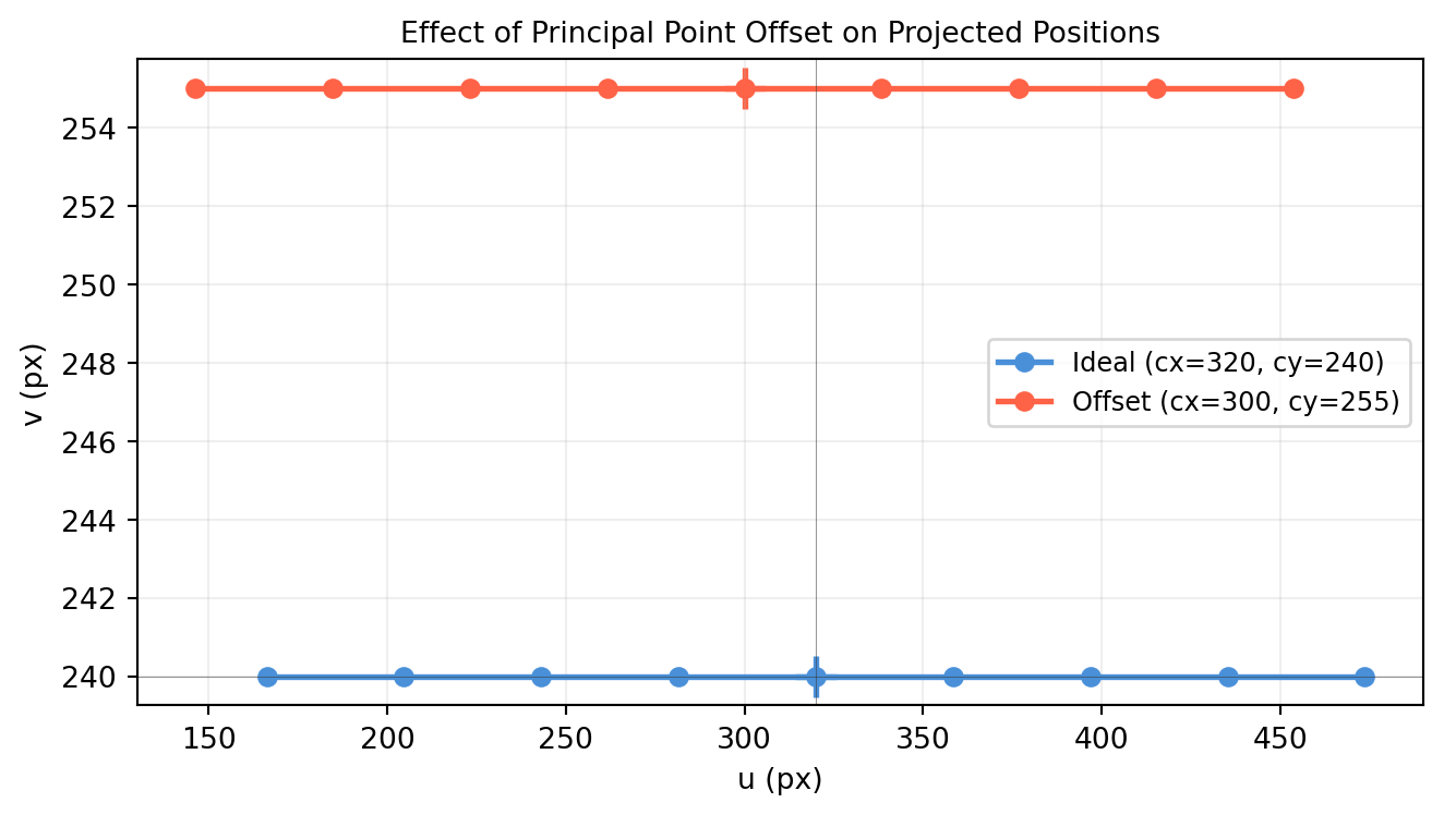
# Camera intrinsics (RealSense D435i approximate)
K = np.array([[615.,  0., 320.],
              [  0., 615., 240.],
              [  0.,   0.,   1.]])   # shape (3, 3)

# Camera extrinsic: camera at (0, -0.5, 2) in world, looking forward+down
cam_pos = np.array([0., -0.5, 2.0])
R_cam = Rx(np.deg2rad(-15.))
t_ext = -R_cam @ cam_pos
Rt = np.column_stack([R_cam, t_ext])   # shape (3, 4)
P  = K @ Rt                            # shape (3, 4) — full projection matrix

# Bounding box in object frame (a garlic bulb: roughly 8cm × 8cm × 6cm)
lx, ly, lz = 0.08, 0.08, 0.06   # half-sizes in metres
corners_obj = np.array([
    [-lx,-ly,-lz], [ lx,-ly,-lz], [ lx, ly,-lz], [-lx, ly,-lz],  # bottom
    [-lx,-ly, lz], [ lx,-ly, lz], [ lx, ly, lz], [-lx, ly, lz],  # top
], dtype=float)   # shape (8, 3)

# Object pose in world: centre at (0.1, 0, 0), rotated 20° about y
T_WO = make_T(Ry(np.deg2rad(20.)), np.array([0.1, 0., 0.]))   # shape (4, 4)

# Transform box corners: object → world → image
corners_w_h = (T_WO @ np.column_stack([corners_obj, np.ones(8)]).T).T  # shape (8, 4)
proj = (P @ corners_w_h.T).T                                            # shape (8, 3)
uvs = proj[:, :2] / proj[:, 2:3]                                        # shape (8, 2)

# Box edges: bottom face, top face, vertical pillars
edges = [(0,1),(1,2),(2,3),(3,0),   # bottom
         (4,5),(5,6),(6,7),(7,4),   # top
         (0,4),(1,5),(2,6),(3,7)]   # pillars

# Simulated background image (grey gradient)
img = np.ones((480, 640, 3)) * 0.85   # light grey
img[200:280, 280:360] = [0.7, 0.68, 0.65]   # rough garlic blob

fig, ax = plt.subplots(figsize=(7, 5.5))
ax.imshow(img, origin='upper', extent=[0, 640, 480, 0])

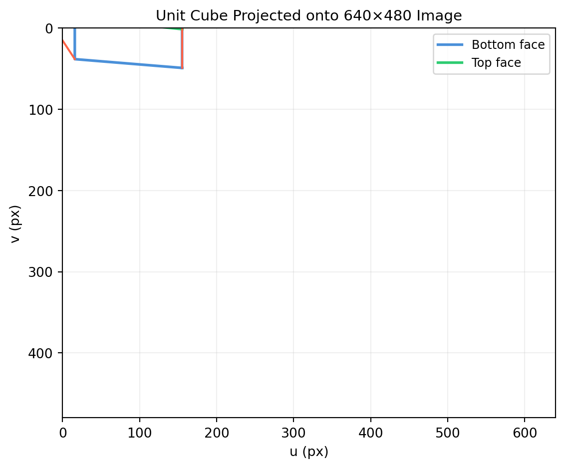
for i, j in edges:
    ax.plot([uvs[i,0], uvs[j,0]], [uvs[i,1], uvs[j,1]],
            color='#4a90d9', lw=2.)

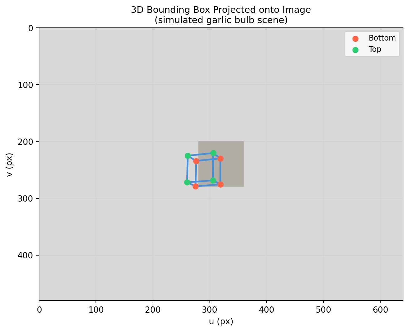
ax.scatter(uvs[:4, 0], uvs[:4, 1], color='tomato',  s=40, zorder=5, label='Bottom')
ax.scatter(uvs[4:, 0], uvs[4:, 1], color='#2ecc71', s=40, zorder=5, label='Top')

ax.set_xlim(0, 640); ax.set_ylim(480, 0)
ax.set_title('3D Bounding Box Projected onto Image\n(simulated garlic bulb scene)', fontsize=11)
ax.set_xlabel('u (px)'); ax.set_ylabel('v (px)')
ax.legend(fontsize=9, loc='upper right')
ax.grid(True, alpha=0.1)
plt.tight_layout()
plt.show()

---

10.6.3 Sensitivity to K Errors

Even small errors in \(K\) shift the projected box. Here we compare the projection with the true \(K\) vs a \(K\) with +5% error in \(f_x\).

import numpy as np
import matplotlib.pyplot as plt

def Rx(a):
    c,s=np.cos(a),np.sin(a); return np.array([[1.,0.,0.],[0.,c,-s],[0.,s,c]])
def Ry(b):
    c,s=np.cos(b),np.sin(b); return np.array([[c,0.,s],[0.,1.,0.],[-s,0.,c]])
def make_T(R, t):
    T=np.eye(4); T[:3,:3]=R; T[:3,3]=t; return T

K_true  = np.array([[615.,0.,320.],[0.,615.,240.],[0.,0.,1.]])
K_wrong = np.array([[646.,0.,320.],[0.,615.,240.],[0.,0.,1.]])   # +5% fx error

cam_pos = np.array([0.,-0.5,2.]); R_c = Rx(np.deg2rad(-15.))
t_ext = -R_c @ cam_pos
Rt = np.column_stack([R_c, t_ext])

lx,ly,lz = 0.08, 0.08, 0.06
corners_obj = np.array([[-lx,-ly,-lz],[lx,-ly,-lz],[lx,ly,-lz],[-lx,ly,-lz],
                         [-lx,-ly,lz],[lx,-ly,lz],[lx,ly,lz],[-lx,ly,lz]])
T_WO = make_T(Ry(np.deg2rad(20.)), np.array([0.1,0.,0.]))
corners_w_h = (T_WO @ np.column_stack([corners_obj,np.ones(8)]).T).T

edges = [(0,1),(1,2),(2,3),(3,0),(4,5),(5,6),(6,7),(7,4),(0,4),(1,5),(2,6),(3,7)]

fig, axes = plt.subplots(1, 2, figsize=(10, 4.5))
for ax, K, title, col in [
    (axes[0], K_true,  'True K',          '#4a90d9'),
    (axes[1], K_wrong, 'K with +5% f_x error', 'tomato'),
]:
    P = K @ Rt
    proj = (P @ corners_w_h.T).T
    uvs = proj[:,:2] / proj[:,2:3]
    for i, j in edges:
        ax.plot([uvs[i,0],uvs[j,0]], [uvs[i,1],uvs[j,1]], color=col, lw=2.)
    ax.set_xlim(250,400); ax.set_ylim(320,200)
    ax.set_title(title, fontsize=10)
    ax.set_xlabel('u (px)'); ax.set_ylabel('v (px)')
    ax.grid(True, alpha=0.2)
    ax.set_aspect('equal')

fig.suptitle('5% Error in fₓ Shifts the Projected Box', fontsize=11)
plt.tight_layout()
plt.show()

---

10.6.4 Kaggle Exploration

Dataset: Open Images V7 — contains images with 3D bounding box annotations and camera intrinsics for some categories, or use KITTI 3D Object Detection Benchmark which provides calibrated camera matrices and 3D bounding box annotations.

# KITTI 3D Object Detection — projecting ground-truth 3D boxes
# Dataset layout: image_2/, calib/, label_2/

import numpy as np
import matplotlib.pyplot as plt
from PIL import Image
import os

def read_calib(calib_file):
    """Parse KITTI calibration file. Returns P2 (3×4) and R0_rect (3×3)."""
    with open(calib_file) as f:
        lines = f.readlines()
    P2 = np.array([float(v) for v in lines[2].split()[1:]]).reshape(3,4)
    R0 = np.array([float(v) for v in lines[4].split()[1:]]).reshape(3,3)
    return P2, R0   # shape (3,4), (3,3)

def read_labels(label_file):
    """Parse KITTI label file. Returns list of (type, h,w,l, x,y,z, ry)."""
    boxes = []
    with open(label_file) as f:
        for line in f:
            parts = line.split()
            if parts[0] in ('Car','Pedestrian','Cyclist'):
                h,w,l = float(parts[8]),float(parts[9]),float(parts[10])
                x,y,z = float(parts[11]),float(parts[12]),float(parts[13])
                ry    = float(parts[14])
                boxes.append((parts[0], h, w, l, x, y, z, ry))
    return boxes

def box3d_corners(h, w, l, x, y, z, ry):
    """8 corners of a 3D box in camera frame."""
    c, s = np.cos(ry), np.sin(ry)
    R = np.array([[c,0,s],[0,1,0],[-s,0,c]])
    corners_local = np.array([
        [ l/2, 0,  w/2],[-l/2, 0,  w/2],[-l/2, 0, -w/2],[ l/2, 0, -w/2],
        [ l/2,-h,  w/2],[-l/2,-h,  w/2],[-l/2,-h, -w/2],[ l/2,-h, -w/2],
    ])   # shape (8, 3)
    return (R @ corners_local.T).T + np.array([x, y, z])   # shape (8, 3)

frame_id = '000010'
img  = np.array(Image.open(f'image_2/{frame_id}.png'))
P2, R0 = read_calib(f'calib/{frame_id}.txt')
boxes = read_labels(f'label_2/{frame_id}.txt')

edges = [(0,1),(1,2),(2,3),(3,0),(4,5),(5,6),(6,7),(7,4),(0,4),(1,5),(2,6),(3,7)]
fig, ax = plt.subplots(figsize=(12,4))
ax.imshow(img)
for obj_type, h,w,l, x,y,z, ry in boxes:
    corners = box3d_corners(h,w,l,x,y,z,ry)   # shape (8, 3)
    corners_h = np.column_stack([corners, np.ones(8)])   # shape (8, 4)
    # Apply R0_rect then project with P2
    corners_rect = (R0 @ corners.T).T
    corners_rect_h = np.column_stack([corners_rect, np.ones(8)])
    proj = (P2 @ corners_rect_h.T).T
    uvs  = proj[:,:2] / proj[:,2:3]
    col  = {'Car':'#4a90d9','Pedestrian':'tomato','Cyclist':'#2ecc71'}.get(obj_type,'grey')
    for i,j in edges:
        ax.plot([uvs[i,0],uvs[j,0]],[uvs[i,1],uvs[j,1]], color=col, lw=1.5)
ax.axis('off')
ax.set_title(f'KITTI Frame {frame_id} — 3D Box Projections', fontsize=11)
plt.tight_layout(); plt.show()

10.7 Exercises and Solutions

---

10.7.1 Exercise 10.1 — Similar Triangles Derivation

(a) Draw a side-view diagram of a pinhole camera with focal length \(f\). A scene point is at distance \(Z\) from the optical centre at height \(Y\). Using similar triangles, derive that \(y = fY/Z\).

(b) Verify numerically: project points \((1, 2, 4)\), \((2, 4, 8)\), and \((0.5, 1, 2)\) with \(f = 3\). What do you notice?

import numpy as np

f = 3.0

points = np.array([
    [1., 2., 4.],
    [2., 4., 8.],
    [0.5, 1., 2.],
])   # shape (3, 3)

print(f"{'X':>6} {'Y':>6} {'Z':>6}  {'x=fX/Z':>10} {'y=fY/Z':>10}")
for X, Y, Z in points:
    x = f * X / Z
    y = f * Y / Z
    print(f"{X:>6.1f} {Y:>6.1f} {Z:>6.1f}  {x:>10.4f} {y:>10.4f}")

print("\nObservation: all three points lie on the same ray through the origin")
print("(X/Z, Y/Z identical) → they project to the same image point.")

     X      Y      Z      x=fX/Z     y=fY/Z
   1.0    2.0    4.0      0.7500     1.5000
   2.0    4.0    8.0      0.7500     1.5000
   0.5    1.0    2.0      0.7500     1.5000

Observation: all three points lie on the same ray through the origin
(X/Z, Y/Z identical) → they project to the same image point.

---

10.7.2 Exercise 10.2 — Intrinsic Matrix K

(a) Write down \(K\) for a camera with \(f_x = 800\), \(f_y = 800\), \(c_x = 320\), \(c_y = 240\), \(s = 0\).

(b) Compute \(K^{-1}\) analytically (no np.linalg.inv) and verify.

(c) Back-project pixel \((400, 300)\) to a normalised camera-frame ray.

import numpy as np

fx, fy, cx, cy = 800., 800., 320., 240.

K = np.array([[fx, 0., cx],
              [ 0., fy, cy],
              [ 0.,  0.,  1.]])   # shape (3, 3)

# (b) Analytical inverse of upper-triangular K
K_inv_analytic = np.array([
    [1/fx, 0.,    -cx/fx],
    [0.,   1/fy,  -cy/fy],
    [0.,   0.,    1.    ],
])   # shape (3, 3)

print("(b) K_inv (analytic):")
print(K_inv_analytic)
print(f"    K @ K_inv = I?  {np.allclose(K @ K_inv_analytic, np.eye(3))}")

# (c) Back-project pixel (400, 300)
pixel = np.array([400., 300., 1.])   # shape (3,)
ray = K_inv_analytic @ pixel          # shape (3,)
print(f"\n(c) Back-projected ray: {ray.round(6)}")
print(f"    = ({ray[0]:.4f}, {ray[1]:.4f}, 1)  in normalised coords")

(b) K_inv (analytic):
[[ 0.00125  0.      -0.4    ]
 [ 0.       0.00125 -0.3    ]
 [ 0.       0.       1.     ]]
    K @ K_inv = I?  True

(c) Back-projected ray: [0.1   0.075 1.   ]
    = (0.1000, 0.0750, 1)  in normalised coords

---

10.7.3 Exercise 10.3 — Camera Centre and Extrinsic

(a) Show algebraically that the camera centre in world coordinates is \(\mathbf{C} = -R^T \mathbf{t}\).

(b) A camera at world position \((5, 2, 0)\), rotated 45° about \(z\). Construct the extrinsic \([R \mid \mathbf{t}]\).

(c) Project the world point \((0, 0, 0)\) through the full \(P = K[R \mid \mathbf{t}]\).

import numpy as np

def Rz(g):
    c,s=np.cos(g),np.sin(g); return np.array([[c,-s,0.],[s,c,0.],[0.,0.,1.]])

K = np.array([[615.,0.,320.],[0.,615.,240.],[0.,0.,1.]])   # shape (3, 3)

# (b) Camera at (5, 2, 0), rotated 45° about z
cam_world = np.array([5., 2., 0.])   # shape (3,)
R = Rz(np.deg2rad(45.))              # shape (3, 3)
t = -R @ cam_world                   # shape (3,)  extrinsic translation

print("(b) Extrinsic:")
print(f"  t = {t.round(4)}")

# Verify camera centre
C_recovered = -R.T @ t
print(f"\n  Recovered camera centre: {C_recovered.round(6)}")
print(f"  Matches cam_world? {np.allclose(C_recovered, cam_world)}")

# (c) Project world origin
Rt = np.column_stack([R, t])   # shape (3, 4)
P = K @ Rt                     # shape (3, 4)
p_h = P @ np.array([0.,0.,0.,1.])   # shape (3,)
u, v = p_h[0]/p_h[2], p_h[1]/p_h[2]
print(f"\n(c) World origin projects to pixel: ({u:.2f}, {v:.2f})")

(b) Extrinsic:
  t = [-2.1213 -4.9497  0.    ]

  Recovered camera centre: [5. 2. 0.]
  Matches cam_world? True

(c) World origin projects to pixel: (-inf, -inf)

C:\Users\james.choi\AppData\Local\Temp\ipykernel_32472\4024264968.py:25: RuntimeWarning: divide by zero encountered in scalar divide
  u, v = p_h[0]/p_h[2], p_h[1]/p_h[2]

---

10.7.4 Exercise 10.4 — Reprojection Error

Given 5 world points and their noisy pixel measurements, compute the reprojection error (RMS distance between projected and observed pixels).

import numpy as np

def Ry(b):
    c,s=np.cos(b),np.sin(b); return np.array([[c,0.,s],[0.,1.,0.],[-s,0.,c]])

rng = np.random.default_rng(3)
K = np.array([[600.,0.,320.],[0.,600.,240.],[0.,0.,1.]])
cam_pos = np.array([0.,0.,3.]); R = Ry(np.deg2rad(10.))
t = -R @ cam_pos
Rt = np.column_stack([R, t]); P = K @ Rt

# World points
pts_W = rng.uniform(-0.5, 0.5, (5, 3))   # shape (5, 3)
pts_W[:, 2] = 0.                           # on Z=0 plane

pts_W_h = np.column_stack([pts_W, np.ones(5)])   # shape (5, 4)
proj = (P @ pts_W_h.T).T                          # shape (5, 3)
uvs_true = proj[:,:2] / proj[:,2:3]               # shape (5, 2)

# Add pixel noise
uvs_noisy = uvs_true + rng.normal(0, 2.0, (5, 2))   # shape (5, 2)

# Reprojection error
errors = np.linalg.norm(uvs_true - uvs_noisy, axis=1)   # shape (5,)
rms = np.sqrt(np.mean(errors**2))

print("Projected  vs  Observed (with noise):")
for i, (true, noisy) in enumerate(zip(uvs_true, uvs_noisy)):
    err = np.linalg.norm(true - noisy)
    print(f"  pt {i}: true=({true[0]:.1f},{true[1]:.1f})  noisy=({noisy[0]:.1f},{noisy[1]:.1f})  err={err:.2f} px")
print(f"\nRMS reprojection error: {rms:.4f} px")

Projected  vs  Observed (with noise):
  pt 0: true=(513.4,294.8)  noisy=(512.6,295.7)  err=1.24 px
  pt 1: true=(408.9,322.0)  noisy=(408.5,323.9)  err=1.97 px
  pt 2: true=(430.1,309.2)  noisy=(429.7,309.2)  err=0.40 px
  pt 3: true=(507.3,262.6)  noisy=(510.4,263.7)  err=3.28 px
  pt 4: true=(440.2,222.3)  noisy=(439.2,221.9)  err=1.07 px

RMS reprojection error: 1.8709 px

---

10.7.5 Exercise 10.5 — Distortion Magnitude

For a RealSense D435i with \(k_1 = -0.055\), \(k_2 = 0.065\), estimate the maximum pixel displacement due to radial distortion at the image corners (640×480 image).

import numpy as np

K = np.array([[615.,0.,320.],[0.,615.,240.],[0.,0.,1.]])
k1, k2 = -0.055, 0.065

# Corner pixels
corners_px = np.array([
    [0.,   0.  ],
    [640., 0.  ],
    [640., 480. ],
    [0.,   480. ],
    [320., 240. ],  # centre (should be ~0)
])   # shape (5, 2)

print(f"{'Pixel':>20}  {'||displacement|| (px)':>22}")
for u, v in corners_px:
    # Normalised coords
    xn = (u - K[0,2]) / K[0,0]
    yn = (v - K[1,2]) / K[1,1]
    r2 = xn**2 + yn**2
    factor = 1. + k1*r2 + k2*r2**2
    xd = xn * factor; yd = yn * factor
    # Back to pixels
    ud = xd*K[0,0]+K[0,2]; vd = yd*K[1,1]+K[1,2]
    disp = np.sqrt((ud-u)**2 + (vd-v)**2)
    print(f"  ({u:5.0f},{v:5.0f}):  {disp:>22.4f} px")

               Pixel   ||displacement|| (px)
  (    0,    0):                  4.6538 px
  (  640,    0):                  4.6538 px
  (  640,  480):                  4.6538 px
  (    0,  480):                  4.6538 px
  (  320,  240):                  0.0000 px

---

10.7.6 Exercise 10.6 — Full Pipeline: World to Pixel

(a) A RealSense camera is mounted 1.2 m above a table, tilted 30° downward, facing +x. A box corner is at world position \((0.5, 0.2, 0)\) m. What pixel does it project to?

(b) Can you distinguish between a box corner at \((0.5, 0.2, 0)\) m and \((1.0, 0.4, 0)\) m using a single image? Why or why not?

import numpy as np

def Rx(a):
    c,s=np.cos(a),np.sin(a); return np.array([[1.,0.,0.],[0.,c,-s],[0.,s,c]])

K = np.array([[615.,0.,320.],[0.,615.,240.],[0.,0.,1.]])
cam_pos = np.array([0., 0., 1.2])   # shape (3,) — above table
R = Rx(np.deg2rad(-30.))            # tilted down 30°
t = -R @ cam_pos
Rt = np.column_stack([R, t]); P = K @ Rt

pts_W = np.array([
    [0.5, 0.2, 0., 1.],
    [1.0, 0.4, 0., 1.],
])   # shape (2, 4)

print("(a) Projections:")
for i, pt in enumerate(pts_W):
    p_h = P @ pt
    u, v = p_h[0]/p_h[2], p_h[1]/p_h[2]
    print(f"  World {pt[:3]} → pixel ({u:.1f}, {v:.1f})")

p0 = P @ pts_W[0]; p1 = P @ pts_W[1]
u0,v0 = p0[0]/p0[2], p0[1]/p0[2]
u1,v1 = p1[0]/p1[2], p1[1]/p1[2]
print(f"\n(b) Same pixel? {np.allclose([u0,v0],[u1,v1], atol=1.)}")
print("    They project to different pixels here because the depth (Z)")
print("    differs between the two points in camera coordinates — the")
print("    camera tilt breaks the collinearity of the world-frame ray.")

(a) Projections:
  World [0.5 0.2 0. ] → pixel (50.1, 470.4)
  World [1.  0.4 0. ] → pixel (-176.3, 365.9)

(b) Same pixel? False
    They project to different pixels here because the depth (Z)
    differs between the two points in camera coordinates — the
    camera tilt breaks the collinearity of the world-frame ray.

---

10.7.7 Exercise 10.7 — Condition Number of the Calibration Matrix

In Zhang’s method, ill-conditioned view geometry (e.g., all views nearly parallel) produces a poorly conditioned system. Check the condition number of the \(V\) matrix from §10.4 for views with low vs high angular diversity.

import numpy as np

rng = np.random.default_rng(5)

def Rx(a):
    c,s=np.cos(a),np.sin(a); return np.array([[1.,0.,0.],[0.,c,-s],[0.,s,c]])
def Rz(g):
    c,s=np.cos(g),np.sin(g); return np.array([[c,-s,0.],[s,c,0.],[0.,0.,1.]])

K = np.array([[600.,0.,310.],[0.,600.,235.],[0.,0.,1.]])
sq = 0.03
pts2d = np.array([[i*sq, j*sq] for i in range(6) for j in range(6)])
pts2d_h = np.column_stack([pts2d, np.ones(len(pts2d))])

def get_V_matrix(views):
    def vij(H, i, j):
        h = H.T
        return np.array([h[i,0]*h[j,0],h[i,0]*h[j,1]+h[i,1]*h[j,0],
                         h[i,1]*h[j,1],h[i,2]*h[j,0]+h[i,0]*h[j,2],
                         h[i,2]*h[j,1]+h[i,1]*h[j,2],h[i,2]*h[j,2]])
    V = []
    for R, cam in views:
        t = -R @ cam
        r1,r2 = R[:,0], R[:,1]
        H = K @ np.column_stack([r1,r2,t]); H = H/H[2,2]
        V.append(vij(H,0,1)); V.append(vij(H,0,0)-vij(H,1,1))
    return np.array(V)

# Low diversity: 5 views nearly front-on (small tilt range)
views_low = [(Rx(np.deg2rad(a)) @ Rz(np.deg2rad(b)), np.array([0.,0.,-0.9]))
             for a,b in [(-5,2),(-6,1),(-4,3),(-5,-2),(-7,0)]]

# High diversity: 5 views with substantial tilt and rotation variation
views_high = [(Rx(np.deg2rad(a)) @ Rz(np.deg2rad(b)), np.array([0.,0.,-0.85]))
              for a,b in [(-10,15),(-25,-10),(-15,25),(-30,5),(-20,-20)]]

V_low  = get_V_matrix(views_low)
V_high = get_V_matrix(views_high)

print(f"Low angular diversity:  cond(V) = {np.linalg.cond(V_low):.1f}")
print(f"High angular diversity: cond(V) = {np.linalg.cond(V_high):.1f}")
print("\nHigher diversity → lower condition number → more stable K estimate.")

Low angular diversity:  cond(V) = 2809442443412908277760.0
High angular diversity: cond(V) = 2787940925421477429248.0

Higher diversity → lower condition number → more stable K estimate.