17 Projections, Pseudoinverse, and Least Squares

17.1 Orthogonal Projection onto a Subspace

The question that launches least squares: given \(A\mathbf{x} = \mathbf{b}\) with no exact solution, what vector in \(\text{Col}(A)\) is closest to \(\mathbf{b}\)? The answer is the orthogonal projection of \(\mathbf{b}\) onto \(\text{Col}(A)\), and the matrix that computes it is the projection matrix \(P\).

17.1.1 Why Exact Solutions Often Do Not Exist

\(A\mathbf{x} = \mathbf{b}\) is solvable only when \(\mathbf{b} \in \text{Col}(A)\). In every real measurement setting – sensor arrays, camera calibration, curve fitting – the number of measurements exceeds the number of unknowns and noise pushes \(\mathbf{b}\) outside \(\text{Col}(A)\). The best achievable result is a vector \(A\hat{\mathbf{x}} \in \text{Col}(A)\) that minimizes \(\|\mathbf{b} - A\mathbf{x}\|_2\).

17.1.2 Deriving the Projection Matrix

Let \(A \in \mathbb{R}^{m \times n}\) have full column rank (\(m > n\), \(\text{rank}(A) = n\)). We seek \(\hat{\mathbf{x}} = \arg\min_\mathbf{x} \|\mathbf{b} - A\mathbf{x}\|_2^2\).

The geometric requirement: the error vector \(\mathbf{e} = \mathbf{b} - A\hat{\mathbf{x}}\) must be orthogonal to every column of \(A\) (otherwise we could reduce the error further by moving along a column direction):

\[A^T \mathbf{e} = \mathbf{0} \;\implies\; A^T(\mathbf{b} - A\hat{\mathbf{x}}) = \mathbf{0} \;\implies\; A^TA\hat{\mathbf{x}} = A^T\mathbf{b}.\]

Since \(A\) has full column rank, \(A^TA \in \mathbb{R}^{n \times n}\) is invertible:

\[\hat{\mathbf{x}} = (A^TA)^{-1}A^T\mathbf{b}.\]

The projection of \(\mathbf{b}\) onto \(\text{Col}(A)\) is then:

\[\boxed{\hat{\mathbf{b}} = A\hat{\mathbf{x}} = A(A^TA)^{-1}A^T\mathbf{b} = P\mathbf{b},} \qquad P = A(A^TA)^{-1}A^T \in \mathbb{R}^{m \times m}.\]

In statistics, \(P\) is called the hat matrix because it puts a hat on \(\mathbf{b}\): \(\hat{\mathbf{b}} = P\mathbf{b}\).

17.1.3 Key Properties

Property	Statement	Why
Symmetric	\(P^T = P\)	\((A(A^TA)^{-1}A^T)^T = A((A^TA)^{-1})^T A^T = A(A^TA)^{-1}A^T\)
Idempotent	\(P^2 = P\)	Projecting an already-projected vector changes nothing
Eigenvalues	only 0 or 1	\(P^2\mathbf{v} = P\mathbf{v}\) implies \(\lambda^2 = \lambda\)
Rank	\(n\)	The column space of \(P\) is \(\text{Col}(A)\)
Complement	\(I - P\) is also a projector	Projects onto \(\text{Col}(A)^\perp\) (left null space of \(A\))

Idempotency proof:

\[P^2 = A(A^TA)^{-1}\underbrace{A^TA(A^TA)^{-1}}_{=I}A^T = A(A^TA)^{-1}A^T = P.\]

The vector \(\mathbf{b} - P\mathbf{b} = (I - P)\mathbf{b}\) is the component of \(\mathbf{b}\) orthogonal to \(\text{Col}(A)\) – it lives in the left null space \(\text{Null}(A^T)\).

17.1.4 Projection onto a Single Vector

The special case \(A = \mathbf{a} \in \mathbb{R}^m\) (a single column) gives a rank-1 projector:

\[P = \frac{\mathbf{a}\mathbf{a}^T}{\mathbf{a}^T\mathbf{a}}, \qquad \hat{\mathbf{b}} = \frac{\mathbf{a}^T\mathbf{b}}{\mathbf{a}^T\mathbf{a}}\,\mathbf{a}.\]

This is the formula from §16.1 written as a matrix operation.

17.1.5 Geometric Visualization

import numpy as np
import matplotlib.pyplot as plt
import matplotlib.patches as mpatches
from matplotlib.patches import FancyArrowPatch

rng = np.random.default_rng(17)

fig, axes = plt.subplots(1, 2, figsize=(12, 5))

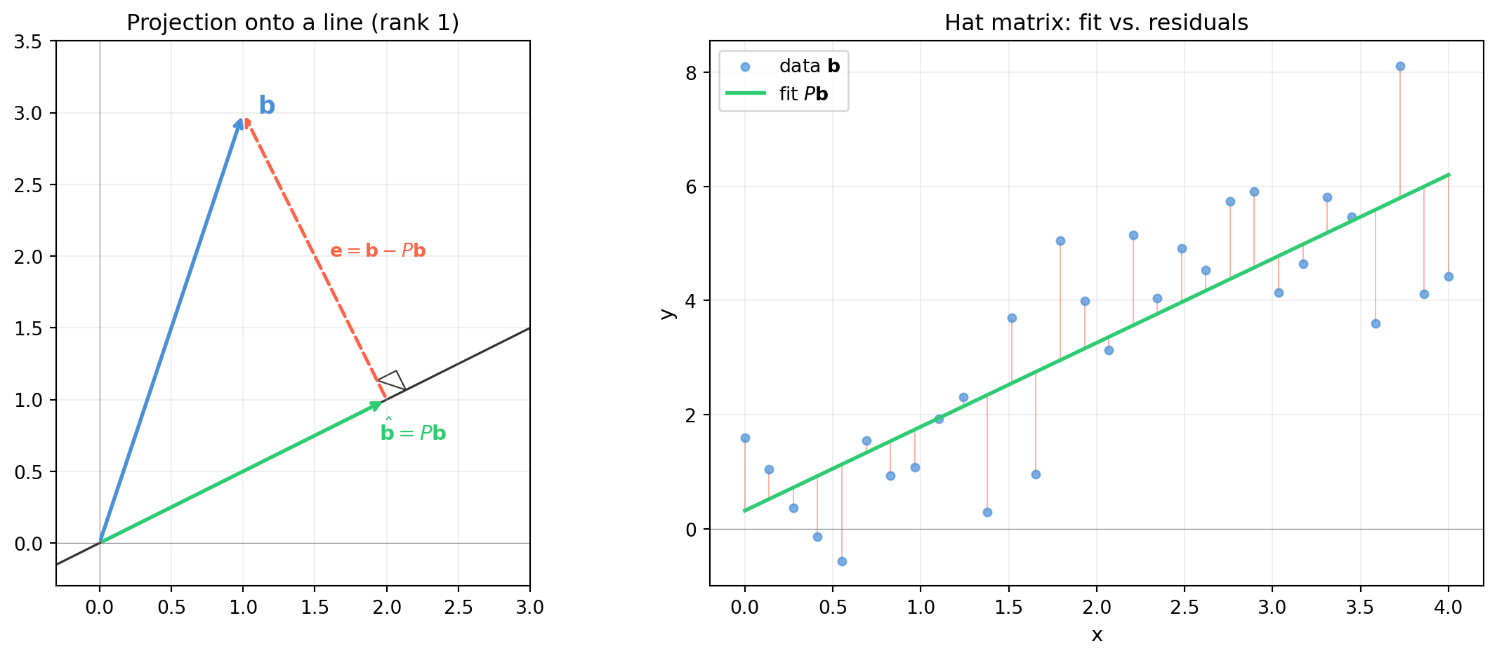
# --- Left: projection in 2D onto a line ---
ax = axes[0]
a = np.array([2.0, 1.0])             # shape (2,) -- column direction
b = np.array([1.0, 3.0])             # shape (2,) -- vector to project

P1 = np.outer(a, a) / float(a @ a)  # shape (2, 2) -- rank-1 projector
b_hat = P1 @ b                       # shape (2,) -- projection
e = b - b_hat                        # shape (2,) -- error (orthogonal to a)

# Line through origin along a
t = np.linspace(-0.5, 2.2, 100)
ax.plot(t * a[0], t * a[1], color='#333333', lw=1.2, zorder=1, label='Col(A)')

ax.annotate('', xy=b, xytext=np.array([0, 0]),
            arrowprops=dict(arrowstyle='->', color='#4a90d9', lw=2))
ax.annotate('', xy=b_hat, xytext=np.array([0, 0]),
            arrowprops=dict(arrowstyle='->', color='#2ecc71', lw=2))
ax.annotate('', xy=b, xytext=b_hat,
            arrowprops=dict(arrowstyle='->', color='tomato', lw=1.8, linestyle='dashed'))

# right-angle mark at b_hat
s = 0.15
v1 = a / np.linalg.norm(a)
v2 = e / np.linalg.norm(e)
corner = b_hat + s * (v1 + v2)
sq = plt.Polygon([b_hat + s * v1, corner, b_hat + s * v2],
                 fill=False, edgecolor='#333333', lw=0.8)
ax.add_patch(sq)

ax.text(b[0] + 0.1, b[1], r'$\mathbf{b}$', fontsize=13, color='#4a90d9')
ax.text(b_hat[0] - 0.05, b_hat[1] - 0.28, r'$\hat{\mathbf{b}} = P\mathbf{b}$',
        fontsize=11, color='#2ecc71')
ax.text((b[0] + b_hat[0]) / 2 + 0.1, (b[1] + b_hat[1]) / 2,
        r'$\mathbf{e} = \mathbf{b} - P\mathbf{b}$', fontsize=10, color='tomato')

ax.set_xlim(-0.3, 3.0)
ax.set_ylim(-0.3, 3.5)
ax.axhline(0, color='#333333', lw=0.4, alpha=0.5)
ax.axvline(0, color='#333333', lw=0.4, alpha=0.5)
ax.set_aspect('equal')
ax.set_title('Projection onto a line (rank 1)', fontsize=12)
ax.grid(alpha=0.2)

# --- Right: hat matrix diagnostics ---
ax2 = axes[1]
m, n = 30, 2                          # overdetermined system
A = np.column_stack([np.ones(m),
                     np.linspace(0, 4, m)])  # shape (30, 2) -- design matrix
b_vec = 1.5 * A[:, 1] + 0.5 + rng.standard_normal(m)  # shape (30,) -- noisy data

P2 = A @ np.linalg.solve(A.T @ A, A.T)   # shape (30, 30)
b_hat2 = P2 @ b_vec                       # shape (30,)
e2 = b_vec - b_hat2                       # shape (30,)

x_vals = A[:, 1]
ax2.scatter(x_vals, b_vec, s=18, color='#4a90d9', alpha=0.7, label=r'data $\mathbf{b}$', zorder=3)
ax2.plot(x_vals, b_hat2, color='#2ecc71', lw=2, label=r'fit $P\mathbf{b}$', zorder=4)
for xi, yi, yhi in zip(x_vals, b_vec, b_hat2):
    ax2.plot([xi, xi], [yi, yhi], color='tomato', lw=0.7, alpha=0.5)

ax2.set_xlabel('x', fontsize=11)
ax2.set_ylabel('y', fontsize=11)
ax2.set_title('Hat matrix: fit vs. residuals', fontsize=12)
ax2.legend(fontsize=10)
ax2.grid(alpha=0.2)
ax2.axhline(0, color='#333333', lw=0.4, alpha=0.5)

fig.tight_layout()
plt.savefig('ch17-least-squares/fig-projection.png', dpi=150, bbox_inches='tight')
plt.show()
print(f"P symmetric:   {np.allclose(P2, P2.T)}")
print(f"P idempotent:  {np.allclose(P2 @ P2, P2)}")
print(f"rank(P):       {np.linalg.matrix_rank(P2)}  (should be {n})")
print(f"e orthogonal to Col(A): max |A^T e| = {np.abs(A.T @ e2).max():.2e}")

P symmetric:   True
P idempotent:  True
rank(P):       2  (should be 2)
e orthogonal to Col(A): max |A^T e| = 6.66e-15

17.1.6 Projection onto a 2-Column Subspace

import numpy as np

rng = np.random.default_rng(171)

# Subspace spanned by two columns in R^5
A = rng.standard_normal((5, 2))       # shape (5, 2)
b = rng.standard_normal(5)            # shape (5,)

# Projection matrix
AtA_inv = np.linalg.inv(A.T @ A)      # shape (2, 2)
P = A @ AtA_inv @ A.T                 # shape (5, 5)

b_hat = P @ b                         # shape (5,)
e = b - b_hat                         # shape (5,)

print(f"P symmetric:   {np.allclose(P, P.T)}")
print(f"P^2 == P:      {np.allclose(P @ P, P)}")
print(f"rank(P):       {np.linalg.matrix_rank(P)}  (should be 2)")
print(f"e in Null(A^T): max |A^T e| = {np.abs(A.T @ e).max():.2e}  (orthogonality check)")
print(f"\n||b||^2 = ||b_hat||^2 + ||e||^2: "
      f"{np.linalg.norm(b)**2:.6f} vs "
      f"{np.linalg.norm(b_hat)**2 + np.linalg.norm(e)**2:.6f}  (Pythagoras)")

P symmetric:   True
P^2 == P:      True
rank(P):       2  (should be 2)
e in Null(A^T): max |A^T e| = 1.25e-16  (orthogonality check)

||b||^2 = ||b_hat||^2 + ||e||^2: 2.755594 vs 2.755594  (Pythagoras)

The Pythagorean identity \(\|\mathbf{b}\|^2 = \|\hat{\mathbf{b}}\|^2 + \|\mathbf{e}\|^2\) holds because \(\hat{\mathbf{b}} \perp \mathbf{e}\).

17.1.7 When \(A^TA\) Is Not Invertible

If \(A\) does not have full column rank, \((A^TA)^{-1}\) does not exist and the formula \(P = A(A^TA)^{-1}A^T\) breaks down. In that case:

The projection still exists (every subspace has a unique orthogonal projector).
But \(\hat{\mathbf{x}}\) is not unique – infinitely many \(\hat{\mathbf{x}}\) achieve the same minimum residual.
The numerically safe approach is to use the pseudoinverse or QR factorization (§17.2, §17.5).

17.1.8 Exercises

17.1.1 Let \(\mathbf{a} = (1, 2, 2)^T\) in \(\mathbb{R}^3\). Write down the \(3 \times 3\) projection matrix \(P\) onto \(\text{span}\{\mathbf{a}\}\). Verify \(P^2 = P\) and \(P^T = P\). What is \(\text{rank}(P)\)?

17.1.2 Let \(A = \begin{bmatrix}1\\2\\2\end{bmatrix}\). Project \(\mathbf{b} = (3, 1, -2)^T\) onto \(\text{Col}(A)\). Then compute \((I - P)\mathbf{b}\) and verify it is orthogonal to \(\mathbf{a}\).

17.1.3 Suppose \(A\) has orthonormal columns (\(A^TA = I\)). Show that \(P = AA^T\). What does this say about the hat matrix when \(A\) comes from QR factorization?

17.1.4 Can the residual \(\mathbf{e} = \mathbf{b} - P\mathbf{b}\) ever be zero for a noisy overdetermined system? Under what condition on \(\mathbf{b}\) does \(P\mathbf{b} = \mathbf{b}\) hold exactly?

17.2 The Pseudoinverse: Moore–Penrose Conditions

When \(A\) is not square, or is square but singular, the ordinary inverse \(A^{-1}\) does not exist. The Moore–Penrose pseudoinverse \(A^+\) generalises the inverse to any matrix while still yielding the minimum-norm least-squares solution. It is defined not by a formula but by four algebraic conditions – and the SVD shows exactly how to compute it.

17.2.1 Four Conditions That Define \(A^+\) Uniquely

Let \(A \in \mathbb{R}^{m \times n}\). The pseudoinverse \(A^+ \in \mathbb{R}^{n \times m}\) is the unique matrix satisfying all four Moore–Penrose conditions:

Condition	Equation	What It Says
(1)	\(AA^+A = A\)	\(A^+\) inverts \(A\) where possible
(2)	\(A^+AA^+ = A^+\)	\(A\) inverts \(A^+\) where possible
(3) Symmetric	\((AA^+)^T = AA^+\)	\(AA^+\) is an orthogonal projector
(4) Symmetric	\((A^+A)^T = A^+A\)	\(A^+A\) is an orthogonal projector

Together these conditions determine \(A^+\) uniquely. The projector \(AA^+\) projects onto \(\text{Col}(A)\); the projector \(A^+A\) projects onto \(\text{Row}(A)\).

When \(A\) is invertible, \(A^+ = A^{-1}\) and all four conditions reduce to \(AA^{-1}=I\).

17.2.2 Computing \(A^+\) via the SVD

The SVD provides the clearest route to \(A^+\). Write \(A = U\Sigma V^T\) where \(U \in \mathbb{R}^{m \times m}\), \(\Sigma \in \mathbb{R}^{m \times n}\), and \(V \in \mathbb{R}^{n \times n}\). Then:

\[\boxed{A^+ = V\Sigma^+ U^T},\]

where \(\Sigma^+\) is obtained from \(\Sigma\) by reciprocating each nonzero singular value and transposing. Zero singular values stay zero – the pseudoinverse does not invert the null space.

Why does this work? Substituting into condition (1): \(AA^+A = U\Sigma V^T \cdot V\Sigma^+ U^T \cdot U\Sigma V^T = U\Sigma\Sigma^+\Sigma V^T = U\Sigma V^T = A\), since \(\Sigma\Sigma^+\Sigma = \Sigma\) on the diagonal. The remaining three conditions follow similarly.

17.2.3 The Minimum-Norm Least-Squares Solution

Given \(A\mathbf{x} \approx \mathbf{b}\), the vector \(\hat{\mathbf{x}} = A^+\mathbf{b}\) simultaneously:

Minimises the residual: \(\|A\hat{\mathbf{x}} - \mathbf{b}\|_2\) is as small as possible.
Has minimum norm: among all minimisers, \(A^+\mathbf{b}\) has the smallest \(\|\cdot\|_2\).

This two-level optimality is what makes \(A^+\) the canonical generalised inverse.

17.2.4 Numerical Rank and the Tolerance Cutoff

In finite precision, “zero” singular values appear as very small numbers. A standard cutoff is:

\[\sigma_i \text{ treated as zero if } \sigma_i < \varepsilon_{\text{mach}} \cdot \sigma_1 \cdot \max(m, n).\]

This is used internally by np.linalg.lstsq and np.linalg.matrix_rank. Naively inverting all singular values amplifies noise in directions corresponding to near-zero \(\sigma_i\).

import numpy as np

rng = np.random.default_rng(22)

# Full-rank case
m, n = 5, 3
A = rng.standard_normal((m, n))    # shape (5, 3)
b = rng.standard_normal(m)         # shape (5,)

A_plus = np.linalg.pinv(A)         # shape (3, 5)

c1 = np.allclose(A @ A_plus @ A, A)
c2 = np.allclose(A_plus @ A @ A_plus, A_plus)
c3 = np.allclose((A @ A_plus).T, A @ A_plus)
c4 = np.allclose((A_plus @ A).T, A_plus @ A)

print("=== Full-rank (5x3) ===")
print(f"AA+A == A:       {c1}")
print(f"A+AA+ == A+:     {c2}")
print(f"(AA+)^T == AA+:  {c3}")
print(f"(A+A)^T == A+A:  {c4}")

x_hat = A_plus @ b                 # shape (3,)
x_ls, _, _, _ = np.linalg.lstsq(A, b, rcond=None)   # shape (3,)
print(f"\n||x_hat - lstsq||: {np.linalg.norm(x_hat - x_ls):.2e}  (should be ~0)")

# Rank-deficient case
print("\n=== Rank-deficient (5x3, rank 2) ===")
A2 = np.column_stack([A[:, 0], A[:, 1], A[:, 0] + A[:, 1]])  # shape (5, 3), rank 2
A_plus2 = np.linalg.pinv(A2)      # shape (3, 5)

x_hat2 = A_plus2 @ b              # shape (3,)  -- minimum-norm minimiser
null_vec = np.array([1.0, 1.0, -1.0])  # shape (3,)  -- in Null(A2)
x_perturbed = x_hat2 + 0.5 * null_vec  # shape (3,)  -- different solution, same residual

print(f"rank(A2):         {np.linalg.matrix_rank(A2)}")
print(f"Residual (A+b):   {np.linalg.norm(A2 @ x_hat2 - b):.6f}")
print(f"Residual (perturbed): {np.linalg.norm(A2 @ x_perturbed - b):.6f}  (same)")
print(f"||x_hat2||:       {np.linalg.norm(x_hat2):.6f}")
print(f"||x_perturbed||:  {np.linalg.norm(x_perturbed):.6f}  (larger)")

=== Full-rank (5x3) ===
AA+A == A:       True
A+AA+ == A+:     True
(AA+)^T == AA+:  True
(A+A)^T == A+A:  True

||x_hat - lstsq||: 2.65e-16  (should be ~0)

=== Rank-deficient (5x3, rank 2) ===
rank(A2):         2
Residual (A+b):   1.612278
Residual (perturbed): 1.612278  (same)
||x_hat2||:       0.769781
||x_perturbed||:  1.158690  (larger)

17.2.5 SVD-Based Construction

import numpy as np

rng = np.random.default_rng(23)

A = rng.standard_normal((4, 3))    # shape (4, 3)
b = rng.standard_normal(4)         # shape (4,)

U, s, Vt = np.linalg.svd(A, full_matrices=False)   # U (4,3), s (3,), Vt (3,3)

print(f"Singular values: {s.round(4)}")

# Build A+ manually: V * diag(1/s) * U^T
# Vt.T has shape (3,3), multiply each row by 1/s_i, then multiply by U^T
A_plus_manual = (Vt.T * (1.0 / s)) @ U.T   # shape (3, 4)

A_plus_np = np.linalg.pinv(A)              # shape (3, 4)
print(f"Manual A+ matches np.linalg.pinv: {np.allclose(A_plus_manual, A_plus_np)}")

P_col = A @ A_plus_manual          # shape (4, 4)  -- projector onto Col(A)
P_row = A_plus_manual @ A          # shape (3, 3)  -- projector onto Row(A)

print(f"AA+ idempotent:  {np.allclose(P_col @ P_col, P_col)}")
print(f"A+A idempotent:  {np.allclose(P_row @ P_row, P_row)}")
print(f"rank(AA+):       {np.linalg.matrix_rank(P_col)}  (= rank(A))")

Singular values: [3.4126 1.145  0.6553]
Manual A+ matches np.linalg.pinv: True
AA+ idempotent:  True
A+A idempotent:  True
rank(AA+):       3  (= rank(A))

17.2.6 Exercises

17.2.1 Let \(A = \begin{bmatrix}1&0\\0&2\\0&0\end{bmatrix}\). Compute \(A^+\) directly from the SVD (singular values are 1 and 2). Verify all four Moore–Penrose conditions by hand.

17.2.2 Show that if \(A\) is square and invertible, then \(A^+ = A^{-1}\). (Use the four conditions.)

17.2.3 Let \(A = \mathbf{u}\sigma\mathbf{v}^T\) be a rank-1 matrix. Show that \(A^+ = \mathbf{v}(1/\sigma)\mathbf{u}^T\). What happens if \(\sigma = 0\)?

17.2.4 In the rank-deficient example above, verify numerically that \(A^+\mathbf{b}\) has smaller norm than \(\mathbf{x}_{\text{perturbed}}\) while achieving the same residual. Explain geometrically why \(A^+\mathbf{b}\) lies in \(\text{Row}(A)\) and the perturbation lies in \(\text{Null}(A)\).

17.3 Left vs. Right Pseudoinverse

The pseudoinverse collapses two qualitatively different situations into one formula. When the system is overdetermined (\(m > n\), more equations than unknowns) the pseudoinverse acts as a left inverse and minimises residual. When the system is underdetermined (\(m < n\), fewer equations than unknowns) it acts as a right inverse and finds the minimum-norm solution. Understanding the distinction is essential for choosing the right solver in practice.

17.3.1 Overdetermined Systems (\(m > n\), Full Column Rank)

When \(A \in \mathbb{R}^{m \times n}\) has \(m > n\) and \(\text{rank}(A) = n\), there is no exact solution to \(A\mathbf{x} = \mathbf{b}\) generically. The pseudoinverse reduces to the left inverse:

\[A^+ = (A^TA)^{-1}A^T \in \mathbb{R}^{n \times m}, \qquad A^+A = I_n.\]

It is a left inverse because applying \(A^+\) to the left recovers \(\mathbf{x}\) from \(A\mathbf{x}\). But \(AA^+ \neq I_m\) – projecting onto \(\text{Col}(A)\) is not the identity when \(\text{Col}(A)\) is a proper subspace of \(\mathbb{R}^m\).

The solution \(\hat{\mathbf{x}} = A^+\mathbf{b} = (A^TA)^{-1}A^T\mathbf{b}\) minimises the residual \(\|A\mathbf{x} - \mathbf{b}\|_2\).

Applications: curve fitting, camera calibration, regression – any problem with more measurements than parameters.

17.3.2 Underdetermined Systems (\(m < n\), Full Row Rank)

When \(A \in \mathbb{R}^{m \times n}\) has \(m < n\) and \(\text{rank}(A) = m\), the system \(A\mathbf{x} = \mathbf{b}\) is consistent but has infinitely many solutions. The pseudoinverse reduces to the right inverse:

\[A^+ = A^T(AA^T)^{-1} \in \mathbb{R}^{n \times m}, \qquad AA^+ = I_m.\]

The solution \(\hat{\mathbf{x}} = A^+\mathbf{b}\) satisfies \(A\hat{\mathbf{x}} = \mathbf{b}\) exactly and lies in \(\text{Row}(A)\) – the null-space component is zero, which is what minimum norm means.

Applications: redundant robot arm inverse kinematics (7-DoF arm, 6-DoF task space), underdetermined linear programs.

17.3.3 Summary

	Overdetermined (\(m > n\))	Underdetermined (\(m < n\))
\(A^+\)	\((A^TA)^{-1}A^T\)	\(A^T(AA^T)^{-1}\)
\(A^+A\)	\(I_n\)	projector onto \(\text{Row}(A)\)
\(AA^+\)	projector onto \(\text{Col}(A)\)	\(I_m\)
Solution property	minimum residual	minimum norm, exact

17.3.4 Overdetermined Example: Linear Regression

import numpy as np

rng = np.random.default_rng(31)

m, n = 20, 2
t = np.linspace(0, 5, m)                      # shape (20,)
A = np.column_stack([np.ones(m), t])          # shape (20, 2)  -- design matrix [1, t]

x_true = np.array([1.5, 0.8])                 # shape (2,)  -- true [intercept, slope]
b = A @ x_true + 0.4 * rng.standard_normal(m) # shape (20,)  -- noisy measurements

# Left pseudoinverse
A_plus_left = np.linalg.inv(A.T @ A) @ A.T   # shape (2, 20)
x_hat = A_plus_left @ b                       # shape (2,)

print("=== Overdetermined (20x2) ===")
print(f"A+A == I_2:    {np.allclose(A_plus_left @ A, np.eye(n))}")
print(f"AA+ == I_20:   {np.allclose(A @ A_plus_left, np.eye(m))}  (not identity)")
print(f"\nx_true: {x_true}")
print(f"x_hat:  {x_hat.round(4)}")
print(f"Residual: {np.linalg.norm(A @ x_hat - b):.4f}")
print(f"rank(AA+): {np.linalg.matrix_rank(A @ A_plus_left)}  (= n = 2, not m = 20)")

=== Overdetermined (20x2) ===
A+A == I_2:    True
AA+ == I_20:   False  (not identity)

x_true: [1.5 0.8]
x_hat:  [1.6641 0.756 ]
Residual: 1.4941
rank(AA+): 2  (= n = 2, not m = 20)

17.3.5 Underdetermined Example: Redundant Arm IK

A planar arm with 5 joints controlling a 2-DoF end-effector: 3 redundant degrees of freedom. The pseudoinverse picks the minimum joint-velocity solution.

import numpy as np

rng = np.random.default_rng(32)

m, n = 2, 5                                   # task dim < joint dim
J = rng.standard_normal((m, n))               # shape (2, 5)  -- Jacobian
p_dot = rng.standard_normal(m)                # shape (2,)   -- desired task velocity

# Right pseudoinverse
J_plus = J.T @ np.linalg.inv(J @ J.T)        # shape (5, 2)

q_dot = J_plus @ p_dot                        # shape (5,)  -- min-norm joint velocity

print("=== Underdetermined (2x5) ===")
print(f"JJ+ == I_2:  {np.allclose(J @ J_plus, np.eye(m))}")
print(f"J+J == I_5:  {np.allclose(J_plus @ J, np.eye(n))}  (not identity)")
print(f"\nTask error ||J q_dot - p_dot||: {np.linalg.norm(J @ q_dot - p_dot):.2e}")
print(f"||q_dot||: {np.linalg.norm(q_dot):.4f}  (minimum norm)")

# Any null-space addition keeps task exact but increases norm
null_vec = np.array([1.0, -1.0, 0.5, -0.5, 0.2])  # shape (5,)
null_part = null_vec - J_plus @ J @ null_vec         # shape (5,)  -- Null(J) component
q_perturbed = q_dot + null_part                      # shape (5,)

print(f"\nPerturbed task error: {np.linalg.norm(J @ q_perturbed - p_dot):.2e}")
print(f"||q_perturbed||: {np.linalg.norm(q_perturbed):.4f}  (larger)")

=== Underdetermined (2x5) ===
JJ+ == I_2:  True
J+J == I_5:  False  (not identity)

Task error ||J q_dot - p_dot||: 5.55e-17
||q_dot||: 0.4141  (minimum norm)

Perturbed task error: 7.30e-16
||q_perturbed||: 1.4386  (larger)

17.3.6 Exercises

17.3.1 Let \(A = \begin{bmatrix}1&2&3\end{bmatrix} \in \mathbb{R}^{1 \times 3}\). Compute the right pseudoinverse \(A^+ = A^T(AA^T)^{-1}\) and find the minimum-norm solution to \(A\mathbf{x} = 1\). Verify \(\mathbf{x}^* \in \text{Row}(A)\).

17.3.2 For the overdetermined case, prove that \(A^+ = (A^TA)^{-1}A^T\) satisfies all four Moore–Penrose conditions when \(A\) has full column rank.

17.3.3 A 4-DoF planar arm controls a 2-DoF end-effector. Write the pseudoinverse IK formula \(\dot{\mathbf{q}} = J^+\dot{\mathbf{p}}\) and explain what happens when \(J\) loses rank at a kinematic singularity.

17.3.4 Show that for any \(A\), the vector \(A^+\mathbf{b}\) is orthogonal to \(\text{Null}(A)\). (Hint: \(A^+A\) is the orthogonal projector onto \(\text{Row}(A)\) and \(A^+\mathbf{b} = A^+A\cdot A^+\mathbf{b}\).)

17.4 The Normal Equations

The normal equations \(A^TA\hat{\mathbf{x}} = A^T\mathbf{b}\) are the classical formulation of least squares. They arise naturally from the orthogonality condition: the residual \(\mathbf{e} = \mathbf{b} - A\hat{\mathbf{x}}\) must be orthogonal to every column of \(A\). Understanding when \(A^TA\) is invertible – and what goes wrong when it is not – is essential before reaching for a solver.

17.4.1 Geometric Derivation

The problem \(\min_\mathbf{x} \|A\mathbf{x} - \mathbf{b}\|_2^2\) has a geometric interpretation: find the point in \(\text{Col}(A)\) closest to \(\mathbf{b}\). The closest point \(\hat{\mathbf{b}} = A\hat{\mathbf{x}}\) is the orthogonal projection of \(\mathbf{b}\) onto \(\text{Col}(A)\), so the error \(\mathbf{e} = \mathbf{b} - A\hat{\mathbf{x}}\) must lie in \(\text{Col}(A)^\perp = \text{Null}(A^T)\):

\[A^T\mathbf{e} = \mathbf{0} \;\implies\; A^T(\mathbf{b} - A\hat{\mathbf{x}}) = \mathbf{0} \;\implies\; \boxed{A^TA\hat{\mathbf{x}} = A^T\mathbf{b}.}\]

This is the normal equations – the residual is “normal” (perpendicular) to the column space.

17.4.2 Algebraic Derivation via Calculus

Expanding the objective \(f(\mathbf{x}) = \|A\mathbf{x} - \mathbf{b}\|_2^2 = \mathbf{x}^TA^TA\mathbf{x} - 2\mathbf{b}^TA\mathbf{x} + \mathbf{b}^T\mathbf{b}\):

\[\nabla_\mathbf{x} f = 2A^TA\mathbf{x} - 2A^T\mathbf{b} = \mathbf{0} \;\implies\; A^TA\hat{\mathbf{x}} = A^T\mathbf{b}.\]

The Hessian is \(2A^TA\), which is positive semidefinite (and positive definite when \(A\) has full column rank), confirming this is a minimum.

17.4.3 When \(A^TA\) Is Invertible

\(A^TA \in \mathbb{R}^{n \times n}\) is invertible if and only if \(A\) has full column rank (\(\text{rank}(A) = n\)). In that case the unique solution is:

\[\hat{\mathbf{x}} = (A^TA)^{-1}A^T\mathbf{b}.\]

Full column rank requires \(m \geq n\) and linearly independent columns. In practice this means the design matrix has no redundant features and enough measurements.

17.4.4 When \(A^TA\) Is Singular

If \(A\) does not have full column rank:

\(A^TA\) is positive semidefinite: some eigenvalues are zero.
The normal equations \(A^TA\hat{\mathbf{x}} = A^T\mathbf{b}\) are still consistent (since \(A^T\mathbf{b} \in \text{Col}(A^T) = \text{Row}(A) = \text{Col}(A^TA)\)).
But the solution is not unique: any \(\hat{\mathbf{x}} + \mathbf{n}\) with \(\mathbf{n} \in \text{Null}(A)\) is also a solution.
The pseudoinverse picks the minimum-norm solution \(\hat{\mathbf{x}} = A^+\mathbf{b}\).

Causes: collinear features (e.g. temperature in Celsius and Kelvin in the same regression), rank-deficient design from insufficient distinct measurements, or a deliberately underdetermined model.

17.4.5 Condition Number and Numerical Concerns

Even when \(A^TA\) is technically invertible, forming it explicitly can cause numerical problems. If \(\text{cond}(A) = \sigma_{\max}/\sigma_{\min}\), then:

\[\text{cond}(A^TA) = \text{cond}(A)^2.\]

Squaring the condition number doubles the number of digits lost to floating-point error. For this reason, the normal equations are recommended only when \(\text{cond}(A)\) is small and forming \(A^TA\) explicitly is acceptable (§17.5).

import numpy as np

rng = np.random.default_rng(41)

# Well-conditioned case
m, n = 10, 3
A = rng.standard_normal((m, n))    # shape (10, 3)
b = rng.standard_normal(m)         # shape (10,)

# Normal equations: solve A^T A x = A^T b
AtA = A.T @ A                      # shape (3, 3)
Atb = A.T @ b                      # shape (3,)
x_ne = np.linalg.solve(AtA, Atb)   # shape (3,)  -- normal equations solution

# Compare with lstsq
x_ls, _, _, _ = np.linalg.lstsq(A, b, rcond=None)   # shape (3,)

sigma = np.linalg.svd(A, compute_uv=False)   # shape (3,)  -- singular values
cond_A = sigma[0] / sigma[-1]

print(f"cond(A):      {cond_A:.2f}")
print(f"cond(A^T A):  {np.linalg.cond(AtA):.2f}  (= cond(A)^2 approximately)")
print(f"||x_ne - lstsq||: {np.linalg.norm(x_ne - x_ls):.2e}  (agree well)")

# Ill-conditioned case: nearly collinear columns
A_ill = np.column_stack([A[:, 0],
                         A[:, 1],
                         A[:, 0] + 1e-6 * rng.standard_normal(m)])  # shape (10, 3)

sigma_ill = np.linalg.svd(A_ill, compute_uv=False)   # shape (3,)
cond_ill = sigma_ill[0] / sigma_ill[-1]

x_ne_ill = np.linalg.solve(A_ill.T @ A_ill, A_ill.T @ b)  # shape (3,)
x_ls_ill, _, _, _ = np.linalg.lstsq(A_ill, b, rcond=None)  # shape (3,)

print(f"\nIll-conditioned:")
print(f"cond(A_ill):         {cond_ill:.2e}")
print(f"cond(A_ill^T A_ill): {np.linalg.cond(A_ill.T @ A_ill):.2e}  (squared!)")
print(f"||x_ne - lstsq||:    {np.linalg.norm(x_ne_ill - x_ls_ill):.2e}  (diverge!)")

cond(A):      1.84
cond(A^T A):  3.38  (= cond(A)^2 approximately)
||x_ne - lstsq||: 4.64e-16  (agree well)

Ill-conditioned:
cond(A_ill):         2.34e+06
cond(A_ill^T A_ill): 5.50e+12  (squared!)
||x_ne - lstsq||:    1.76e+01  (diverge!)

17.4.6 Visualising Orthogonality of the Residual

import numpy as np
import matplotlib.pyplot as plt

rng = np.random.default_rng(42)

m = 15
t = np.linspace(0, 3, m)                      # shape (15,)
A = np.column_stack([np.ones(m), t])          # shape (15, 2)
b = 2.0 + 1.2 * t + 0.5 * rng.standard_normal(m)  # shape (15,)

# Solve normal equations
x_hat = np.linalg.solve(A.T @ A, A.T @ b)    # shape (2,)
b_hat = A @ x_hat                             # shape (15,)
e = b - b_hat                                 # shape (15,)

fig, axes = plt.subplots(1, 2, figsize=(12, 4))

# Left: data and fit
ax = axes[0]
ax.scatter(t, b, s=20, color='#4a90d9', alpha=0.8, label='data', zorder=3)
ax.plot(t, b_hat, color='#2ecc71', lw=2, label='fit', zorder=4)
for xi, yi, yhi in zip(t, b, b_hat):
    ax.plot([xi, xi], [yi, yhi], color='tomato', lw=0.8, alpha=0.5)
ax.set_xlabel('t', fontsize=11)
ax.set_ylabel('y', fontsize=11)
ax.set_title('Normal equations fit and residuals', fontsize=11)
ax.legend(fontsize=10)
ax.grid(alpha=0.2)

# Right: residuals vs t and vs fitted values (should be uncorrelated)
ax2 = axes[1]
ax2.scatter(b_hat, e, s=20, color='tomato', alpha=0.8, zorder=3)
ax2.axhline(0, color='#333333', lw=1)
ax2.set_xlabel(r'Fitted value $\hat{b}$', fontsize=11)
ax2.set_ylabel(r'Residual $e$', fontsize=11)
ax2.set_title('Residual vs. fitted (orthogonality check)', fontsize=11)
ax2.grid(alpha=0.2)

fig.tight_layout()
plt.savefig('ch17-least-squares/fig-normal-equations.png', dpi=150, bbox_inches='tight')
plt.show()

# Verify orthogonality: A^T e should be zero
print(f"A^T e (should be ~0): {(A.T @ e).round(8)}")
print(f"Corr(b_hat, e): {np.corrcoef(b_hat, e)[0,1]:.2e}  (should be ~0)")

A^T e (should be ~0): [0. 0.]
Corr(b_hat, e): -3.00e-16  (should be ~0)

17.4.7 Exercises

17.4.1 Derive the normal equations by setting \(\nabla_\mathbf{x}\|A\mathbf{x} - \mathbf{b}\|_2^2 = 0\). Identify the Hessian and explain why the critical point is a minimum (not a saddle) when \(A\) has full column rank.

17.4.2 Let \(A \in \mathbb{R}^{3 \times 2}\) be the matrix with columns \((1,1,0)^T\) and \((0,1,1)^T\), and let \(\mathbf{b} = (1,2,3)^T\). Solve the normal equations by hand to find \(\hat{\mathbf{x}}\) and the projection \(\hat{\mathbf{b}} = A\hat{\mathbf{x}}\).

17.4.3 Show that if \(\mathbf{b} \in \text{Col}(A)\), then the normal equations give \(A\hat{\mathbf{x}} = \mathbf{b}\) exactly and \(\mathbf{e} = \mathbf{0}\).

17.4.4 Explain, using eigenvalues, why \(\text{cond}(A^TA) = \text{cond}(A)^2\). In double precision, roughly how large can \(\text{cond}(A)\) be before the normal equations lose all accuracy?

17.5 Solver Comparison: QR vs. SVD vs. Normal Equations

Three algorithms solve \(\min_\mathbf{x}\|A\mathbf{x}-\mathbf{b}\|_2^2\): the normal equations, QR factorisation, and the SVD. They give the same answer on well-conditioned problems but diverge dramatically on ill-conditioned or rank-deficient ones. Knowing which to reach for – and why – separates reliable implementations from fragile ones.

17.5.1 The Three Approaches

Normal equations. Solve \(A^TA\hat{\mathbf{x}} = A^T\mathbf{b}\) via Cholesky factorisation of \(A^TA\). Cost: \(O(mn^2 + n^3/3)\). Pros: simple, fast when \(\text{cond}(A)\) is small. Cons: squares the condition number; fails or gives garbage when \(A\) is nearly rank-deficient.

QR factorisation. Factor \(A = QR\) (Householder, §16.5), then solve \(R\hat{\mathbf{x}} = Q^T\mathbf{b}\) by back-substitution. Cost: \(O(2mn^2 - 2n^3/3)\). Pros: backward stable; does not square the condition number. Cons: cannot detect rank deficiency; breaks when \(R\) is singular.

SVD. Factor \(A = U\Sigma V^T\), then \(\hat{\mathbf{x}} = V\Sigma^+U^T\mathbf{b}\). Cost: \(O(mn^2 + n^3)\) (more expensive). Pros: handles rank deficiency exactly; exposes the complete numerical rank structure via singular values; most robust. Cons: slowest; overkill for well-conditioned problems.

17.5.2 Accuracy on an Ill-Conditioned Problem

import numpy as np

rng = np.random.default_rng(51)

m, n = 30, 5
# Build a matrix with a wide range of singular values
U, _ = np.linalg.qr(rng.standard_normal((m, m)))  # shape (30, 30) -- random orthogonal
V, _ = np.linalg.qr(rng.standard_normal((n, n)))  # shape (5, 5)  -- random orthogonal
sigma = np.array([1e4, 1e2, 1e1, 1.0, 1e-4])      # shape (5,)  -- cond = 1e8
Sigma = np.zeros((m, n))                            # shape (30, 5)
Sigma[:n, :n] = np.diag(sigma)
A = U[:, :n] @ Sigma[:n, :] @ V.T                  # shape (30, 5)  -- cond ~ 1e8

x_true = rng.standard_normal(n)                    # shape (5,)
b = A @ x_true + 1e-3 * rng.standard_normal(m)    # shape (30,)  -- small noise

print(f"cond(A):       {np.linalg.cond(A):.2e}")
print(f"cond(A^T A):   {np.linalg.cond(A.T @ A):.2e}")

# Method 1: normal equations
try:
    x_ne = np.linalg.solve(A.T @ A, A.T @ b)      # shape (5,)
    err_ne = np.linalg.norm(x_ne - x_true)
except np.linalg.LinAlgError:
    err_ne = float('inf')

# Method 2: QR
Q, R = np.linalg.qr(A, mode='reduced')            # Q (30,5), R (5,5)
x_qr = np.linalg.solve(R, Q.T @ b)                # shape (5,)
err_qr = np.linalg.norm(x_qr - x_true)

# Method 3: SVD (pseudoinverse)
x_svd = np.linalg.pinv(A) @ b                     # shape (5,)
err_svd = np.linalg.norm(x_svd - x_true)

# Method 4: lstsq (uses SVD internally)
x_ls, _, _, _ = np.linalg.lstsq(A, b, rcond=None) # shape (5,)
err_ls = np.linalg.norm(x_ls - x_true)

print(f"\n||x_ne - x_true||:   {err_ne:.2e}")
print(f"||x_qr - x_true||:   {err_qr:.2e}")
print(f"||x_svd - x_true||:  {err_svd:.2e}")
print(f"||x_ls - x_true||:   {err_ls:.2e}")
print("\n(Normal eqs degrade; QR holds; SVD/lstsq most stable)")

cond(A):       1.00e+08
cond(A^T A):   1.28e+16

||x_ne - x_true||:   6.12e+00
||x_qr - x_true||:   4.16e+00
||x_svd - x_true||:  4.16e+00
||x_ls - x_true||:   4.16e+00

(Normal eqs degrade; QR holds; SVD/lstsq most stable)

17.5.3 Rank-Deficient Case

When \(A\) loses rank, normal equations fail, QR produces an ill-conditioned \(R\) (and may error), but SVD handles the situation cleanly by zeroing out near-zero singular values.

import numpy as np

rng = np.random.default_rng(52)

m, n = 20, 4
A_full = rng.standard_normal((m, n))             # shape (20, 4)
# Make rank 3: fourth column = linear combination of first three
A = np.column_stack([A_full[:, :3],
                     A_full[:, 0] + 0.5 * A_full[:, 1]])  # shape (20, 4), rank 3

b = rng.standard_normal(m)                       # shape (20,)

# SVD approach handles rank deficiency
x_svd = np.linalg.pinv(A) @ b                   # shape (4,)  -- min-norm least-squares
x_ls, _, rank_ls, sv = np.linalg.lstsq(A, b, rcond=None)   # shape (4,)

print(f"rank(A):                {np.linalg.matrix_rank(A)}  (should be 3)")
print(f"lstsq detected rank:    {rank_ls}")
print(f"Singular values:        {sv.round(4)}")
print(f"\nResidual (svd):  {np.linalg.norm(A @ x_svd - b):.6f}")
print(f"Residual (lstsq): {np.linalg.norm(A @ x_ls - b):.6f}")
print(f"||x_svd - x_ls||: {np.linalg.norm(x_svd - x_ls):.2e}  (same min-norm solution)")

rank(A):                3  (should be 3)
lstsq detected rank:    3
Singular values:        [6.8709 4.4366 4.2115 0.    ]

Residual (svd):  3.973594
Residual (lstsq): 3.973594
||x_svd - x_ls||: 1.85e-16  (same min-norm solution)

17.5.4 Decision Guide

Situation	Recommended Solver
Well-conditioned, \(m \gg n\), speed matters	Normal equations + Cholesky
General overdetermined, moderate \(\text{cond}(A)\)	QR (`np.linalg.lstsq`)
Rank-deficient or very ill-conditioned	SVD / `np.linalg.lstsq` with `rcond`
Real-time IK (small \(n\), latency-critical)	QR or pre-computed pseudoinverse
Camera calibration (batch, need robustness)	SVD-based `cv2.calibrateCamera`
Large sparse \(A\) (\(n > 10^5\))	Iterative: CG, LSQR (§17.8)

The rule of thumb: use np.linalg.lstsq by default (it uses LAPACK’s dgelsd, SVD-based). Switch to QR for speed when you know \(A\) is well-conditioned. Never use normal equations when \(\text{cond}(A) > 10^7\) in double precision.

17.5.5 Visualising the Effect of Ill-Conditioning

import numpy as np
import matplotlib.pyplot as plt

rng = np.random.default_rng(53)

# Sweep condition numbers and measure error amplification
cond_vals = np.logspace(1, 12, 20)   # shape (20,)
err_ne = []
err_qr = []
err_svd = []

m, n = 20, 3

for cond_target in cond_vals:
    U, _ = np.linalg.qr(rng.standard_normal((m, m)))   # shape (20, 20)
    V, _ = np.linalg.qr(rng.standard_normal((n, n)))   # shape (3, 3)
    sv = np.array([1.0, 1.0 / np.sqrt(cond_target), 1.0 / cond_target])  # shape (3,)
    Sigma = np.zeros((m, n))           # shape (20, 3)
    Sigma[:n, :n] = np.diag(sv)
    A = U[:, :n] @ Sigma[:n, :] @ V.T  # shape (20, 3)

    x_true = rng.standard_normal(n)    # shape (3,)
    noise = 1e-10 * rng.standard_normal(m)  # shape (20,)
    b = A @ x_true + noise

    x_ne = np.linalg.lstsq(A.T @ A, A.T @ b, rcond=None)[0]  # normal eqs
    Q_m, R_m = np.linalg.qr(A, mode='reduced')
    x_qr = np.linalg.solve(R_m, Q_m.T @ b)
    x_sv = np.linalg.pinv(A) @ b

    err_ne.append(np.linalg.norm(x_ne - x_true))
    err_qr.append(np.linalg.norm(x_qr - x_true))
    err_svd.append(np.linalg.norm(x_sv - x_true))

fig, ax = plt.subplots(figsize=(8, 5))
ax.loglog(cond_vals, err_ne, color='tomato', lw=2, label='Normal equations')
ax.loglog(cond_vals, err_qr, color='#4a90d9', lw=2, label='QR')
ax.loglog(cond_vals, err_svd, color='#2ecc71', lw=2, label='SVD')
ax.set_xlabel('cond(A)', fontsize=11)
ax.set_ylabel(r'$\|x_{hat} - x_{true}\|_2$', fontsize=11)
ax.set_title('Solver accuracy vs. condition number', fontsize=12)
ax.legend(fontsize=10)
ax.grid(alpha=0.2, which='both')
fig.tight_layout()
plt.savefig('ch17-least-squares/fig-solver-comparison.png', dpi=150, bbox_inches='tight')
plt.show()

17.5.6 Exercises

17.5.1 For \(A = \begin{bmatrix}1&1\\1&1+\varepsilon\end{bmatrix}\) with small \(\varepsilon > 0\), compute \(\text{cond}(A)\) and \(\text{cond}(A^TA)\) symbolically. What happens as \(\varepsilon \to 0\)?

17.5.2 Show algebraically that solving via QR (\(R\hat{\mathbf{x}} = Q^T\mathbf{b}\)) is equivalent to the normal equations. Why is QR more accurate despite the equivalence?

17.5.3 Explain why np.linalg.lstsq uses SVD by default and what the rcond parameter controls. What is a good value of rcond for double-precision input with \(\text{cond}(A) \approx 10^6\)?

17.5.4 When is it safe to use the normal equations? Give a concrete example from robotics or machine learning where forming \(A^TA\) explicitly is standard practice.

17.6 Weighted and Constrained Least Squares

Standard least squares treats every residual equally. In practice, measurements have different noise levels and solutions must sometimes satisfy hard constraints. Weighted least squares handles the first; Lagrange multipliers handle the second. Both reduce to a standard linear solve.

17.6.1 Weighted Least Squares

When measurement \(i\) has standard deviation \(\sigma_i\), the appropriate objective is the weighted sum of squared residuals:

\[\min_\mathbf{x} \sum_{i=1}^m w_i (b_i - \mathbf{a}_i^T\mathbf{x})^2 = \min_\mathbf{x} (A\mathbf{x} - \mathbf{b})^T W (A\mathbf{x} - \mathbf{b}),\]

where \(W = \text{diag}(w_1, \ldots, w_m) \succ 0\) is the weight matrix. Standard choice: \(w_i = 1/\sigma_i^2\) (inverse variance weighting), which is maximum-likelihood estimation under independent Gaussian noise.

Reduction to standard form. Let \(W = L^TL\) (e.g. \(L = \text{diag}(\sqrt{w_i})\)). Then:

\[(A\mathbf{x} - \mathbf{b})^TW(A\mathbf{x} - \mathbf{b}) = \|LA\mathbf{x} - L\mathbf{b}\|_2^2.\]

This is ordinary least squares with \(\tilde{A} = LA\) and \(\tilde{\mathbf{b}} = L\mathbf{b}\). The weighted normal equations are:

\[\boxed{A^TWA\hat{\mathbf{x}} = A^TW\mathbf{b}.}\]

17.6.2 Constrained Least Squares via Lagrange Multipliers

Equality-constrained problem: minimise \(\|A\mathbf{x} - \mathbf{b}\|_2^2\) subject to \(C\mathbf{x} = \mathbf{d}\), where \(C \in \mathbb{R}^{p \times n}\) and \(p < n\).

Form the Lagrangian:

\[\mathcal{L}(\mathbf{x}, \boldsymbol{\lambda}) = \|A\mathbf{x} - \mathbf{b}\|_2^2 + \boldsymbol{\lambda}^T(C\mathbf{x} - \mathbf{d}).\]

Setting \(\nabla_\mathbf{x}\mathcal{L} = 0\) and \(\nabla_{\boldsymbol{\lambda}}\mathcal{L} = 0\):

\[\begin{bmatrix}2A^TA & C^T \\ C & 0\end{bmatrix} \begin{bmatrix}\hat{\mathbf{x}} \\ \boldsymbol{\lambda}\end{bmatrix} = \begin{bmatrix}2A^T\mathbf{b} \\ \mathbf{d}\end{bmatrix}.\]

This KKT system is a \((n+p) \times (n+p)\) saddle-point linear system. It is solvable when \(A\) has full column rank and \(C\) has full row rank.

17.6.3 Weighted Least Squares Example: Depth Fitting with Heteroscedastic Noise

import numpy as np
import matplotlib.pyplot as plt

rng = np.random.default_rng(61)

m = 30
t = np.linspace(0.5, 5.0, m)           # shape (30,)  -- depth in meters
A = np.column_stack([np.ones(m), t])   # shape (30, 2)  -- [1, t] design matrix

x_true = np.array([0.2, 0.15])         # shape (2,)  -- true coefficients
sigma = 0.05 + 0.12 * t                # shape (30,)  -- noise grows with depth
b = A @ x_true + sigma * rng.standard_normal(m)  # shape (30,)

# Ordinary least squares
x_ols = np.linalg.solve(A.T @ A, A.T @ b)   # shape (2,)

# Weighted least squares: w_i = 1/sigma_i^2
w = 1.0 / sigma**2                           # shape (30,)
W = np.diag(w)                               # shape (30, 30)
x_wls = np.linalg.solve(A.T @ W @ A, A.T @ W @ b)  # shape (2,)

# Alternatively: scale A and b by sqrt(w_i), then use OLS
sqrtw = np.sqrt(w)                           # shape (30,)
A_tilde = A * sqrtw[:, None]                 # shape (30, 2)
b_tilde = b * sqrtw                          # shape (30,)
x_wls_v2 = np.linalg.solve(A_tilde.T @ A_tilde, A_tilde.T @ b_tilde)  # shape (2,)

print("=== Weighted Least Squares ===")
print(f"x_true:  {x_true}")
print(f"x_ols:   {x_ols.round(4)}")
print(f"x_wls:   {x_wls.round(4)}")
print(f"x_wls_v2:{x_wls_v2.round(4)}  (equivalent via scaling)")

fig, ax = plt.subplots(figsize=(8, 5))
ax.scatter(t, b, s=20, color='#4a90d9', alpha=0.6, label='data', zorder=3)
ax.errorbar(t, b, yerr=sigma, fmt='none', color='#4a90d9', alpha=0.2, lw=0.8)
ax.plot(t, A @ x_ols, color='tomato', lw=2, label='OLS fit')
ax.plot(t, A @ x_wls, color='#2ecc71', lw=2, label='WLS fit')
ax.plot(t, A @ x_true, color='#333333', lw=1.5, linestyle='--', label='truth')
ax.set_xlabel('t (depth)', fontsize=11)
ax.set_ylabel('b', fontsize=11)
ax.set_title('OLS vs. WLS: heteroscedastic noise', fontsize=12)
ax.legend(fontsize=10)
ax.grid(alpha=0.2)
fig.tight_layout()
plt.savefig('ch17-least-squares/fig-weighted-ls.png', dpi=150, bbox_inches='tight')
plt.show()

=== Weighted Least Squares ===
x_true:  [0.2  0.15]
x_ols:   [0.3933 0.0612]
x_wls:   [0.1658 0.1542]
x_wls_v2:[0.1658 0.1542]  (equivalent via scaling)

17.6.4 Constrained Least Squares Example: Sum-to-Zero Constraint

import numpy as np

rng = np.random.default_rng(62)

# Overdetermined system with a linear equality constraint
m, n = 15, 3
A = rng.standard_normal((m, n))         # shape (15, 3)
b = rng.standard_normal(m)              # shape (15,)

# Constraint: x_1 + x_2 + x_3 = 1  (e.g. simplex-like)
C = np.array([[1.0, 1.0, 1.0]])         # shape (1, 3)
d = np.array([1.0])                     # shape (1,)

p = C.shape[0]                          # number of constraints = 1

# Build KKT system
# [2 A^T A  C^T] [x     ]   [2 A^T b]
# [C        0  ] [lambda] = [d      ]
AtA = 2.0 * A.T @ A                     # shape (3, 3)
Atb = 2.0 * A.T @ b                     # shape (3,)

KKT = np.block([
    [AtA,         C.T              ],
    [C,           np.zeros((p, p)) ]
])                                       # shape (4, 4)

rhs = np.concatenate([Atb, d])           # shape (4,)

sol = np.linalg.solve(KKT, rhs)         # shape (4,)
x_constrained = sol[:n]                  # shape (3,)
lam = sol[n:]                            # shape (1,)  -- Lagrange multiplier

# Unconstrained solution for comparison
x_unconstrained = np.linalg.solve(A.T @ A, A.T @ b)  # shape (3,)

print("=== Constrained Least Squares ===")
print(f"x_constrained:    {x_constrained.round(4)}")
print(f"Constraint C x:   {(C @ x_constrained).item():.6f}  (should be 1.0)")
print(f"Lagrange mult:    {lam.item():.4f}")
print(f"\nx_unconstrained:  {x_unconstrained.round(4)}")
print(f"Constraint C x:   {(C @ x_unconstrained).item():.4f}  (unconstrained, != 1)")
print(f"\nResiduals -- constrained:   {np.linalg.norm(A @ x_constrained - b):.6f}")
print(f"           unconstrained: {np.linalg.norm(A @ x_unconstrained - b):.6f}  (smaller, as expected)")

=== Constrained Least Squares ===
x_constrained:    [0.1423 0.6935 0.1641]
Constraint C x:   1.000000  (should be 1.0)
Lagrange mult:    -11.4740

x_unconstrained:  [-0.4956  0.3706  0.0215]
Constraint C x:   -0.1036  (unconstrained, != 1)

Residuals -- constrained:   4.196709
           unconstrained: 3.358757  (smaller, as expected)

17.6.5 Exercises

17.6.1 Show that the weighted normal equations \(A^TWA\hat{\mathbf{x}} = A^TW\mathbf{b}\) can be derived by defining \(\tilde{A} = W^{1/2}A\) and \(\tilde{\mathbf{b}} = W^{1/2}\mathbf{b}\) and writing the standard normal equations for \(\tilde{A}\mathbf{x} = \tilde{\mathbf{b}}\).

17.6.2 A GPS receiver gives three position measurements with standard deviations \(\sigma_1 = 1\text{ m}\), \(\sigma_2 = 2\text{ m}\), \(\sigma_3 = 0.5\text{ m}\). Set up the weighted least squares problem to estimate a single position \(x\) from the three measurements. Solve and interpret the result.

17.6.3 Derive the KKT system for equality-constrained least squares by differentiating the Lagrangian \(\mathcal{L}(\mathbf{x}, \boldsymbol{\lambda}) = \|A\mathbf{x} - \mathbf{b}\|^2 + \boldsymbol{\lambda}^T(C\mathbf{x} - \mathbf{d})\) with respect to \(\mathbf{x}\) and \(\boldsymbol{\lambda}\).

17.6.4 In the constrained example above, the constrained residual is larger than the unconstrained residual. Prove this is always the case: the optimal unconstrained residual \(\leq\) optimal constrained residual.

17.7 Regularized Least Squares

When \(A\) is ill-conditioned or rank-deficient, the least-squares solution is sensitive to noise: tiny perturbations in \(\mathbf{b}\) can produce wildly different \(\hat{\mathbf{x}}\). Regularisation adds a penalty on \(\|\mathbf{x}\|\) to stabilise the solution, trading a small increase in bias for a large reduction in variance.

17.7.1 Tikhonov Regularisation (Ridge Regression)

The Tikhonov or ridge problem is:

\[\min_\mathbf{x} \|A\mathbf{x} - \mathbf{b}\|_2^2 + \lambda\|\mathbf{x}\|_2^2, \qquad \lambda > 0.\]

Setting the gradient to zero:

\[2A^T(A\mathbf{x} - \mathbf{b}) + 2\lambda\mathbf{x} = \mathbf{0} \;\implies\; \boxed{(A^TA + \lambda I)\hat{\mathbf{x}}_\lambda = A^T\mathbf{b}.}\]

The matrix \(A^TA + \lambda I\) is always positive definite (eigenvalues \(\geq \lambda > 0\)), so the solution is always unique regardless of the rank of \(A\).

17.7.2 Effect on Singular Values

Using the SVD \(A = U\Sigma V^T\), the Tikhonov solution has a clean expression:

\[\hat{\mathbf{x}}_\lambda = V \underbrace{\text{diag}\!\left(\frac{\sigma_i}{\sigma_i^2 + \lambda}\right)}_{\text{regularised gain}} U^T \mathbf{b}.\]

Compare to the pseudoinverse: \(A^+\mathbf{b} = V\,\text{diag}(1/\sigma_i)\,U^T\mathbf{b}\). The regularised gain \(\sigma_i/(\sigma_i^2 + \lambda)\) is:

\(\approx 1/\sigma_i\) when \(\sigma_i \gg \sqrt{\lambda}\) (large singular values: unaffected)
\(\approx \sigma_i/\lambda \approx 0\) when \(\sigma_i \ll \sqrt{\lambda}\) (small singular values: suppressed)

Tikhonov regularisation shrinks the contribution of directions with small singular values without discarding them entirely, unlike the hard cutoff in pinv.

17.7.3 Bias–Variance Interpretation

In statistics, \(\hat{\mathbf{x}}_\lambda\) introduces bias (\(\hat{\mathbf{x}}_\lambda \neq \mathbf{x}_{\text{true}}\) even with no noise) in exchange for lower variance (less sensitivity to noise). Choosing \(\lambda\) is a bias–variance trade-off:

\(\lambda \to 0\): \(\hat{\mathbf{x}}_\lambda \to A^+\mathbf{b}\) (unregularised, low bias, high variance)
\(\lambda \to \infty\): \(\hat{\mathbf{x}}_\lambda \to \mathbf{0}\) (all shrinkage, high bias, zero variance)

Cross-validation selects \(\lambda\) by evaluating hold-out prediction error.

17.7.4 Numerical Demonstration

import numpy as np
import matplotlib.pyplot as plt

rng = np.random.default_rng(71)

m, n = 40, 8
# Design matrix with moderate conditioning
A = rng.standard_normal((m, n))    # shape (40, 8)

# True solution has unit norm
x_true = rng.standard_normal(n)    # shape (8,)
x_true /= np.linalg.norm(x_true)

noise_level = 0.5
b = A @ x_true + noise_level * rng.standard_normal(m)  # shape (40,)

lambdas = np.logspace(-4, 4, 200)  # shape (200,)  -- regularisation sweep

# Compute solutions for each lambda
errors = []
norms = []

AtA = A.T @ A                      # shape (8, 8)
Atb = A.T @ b                      # shape (8,)

for lam in lambdas:
    x_lam = np.linalg.solve(AtA + lam * np.eye(n), Atb)  # shape (8,)
    errors.append(np.linalg.norm(x_lam - x_true))
    norms.append(np.linalg.norm(x_lam))

errors = np.array(errors)   # shape (200,)
norms = np.array(norms)     # shape (200,)

best_idx = np.argmin(errors)
best_lam = lambdas[best_idx]
print(f"Best lambda:    {best_lam:.4f}")
print(f"Min error:      {errors[best_idx]:.4f}")

fig, axes = plt.subplots(1, 2, figsize=(12, 4))

ax = axes[0]
ax.semilogx(lambdas, errors, color='#4a90d9', lw=2)
ax.axvline(best_lam, color='tomato', lw=1.5, linestyle='--', label=f'best lambda={best_lam:.3f}')
ax.set_xlabel(r'$\lambda$', fontsize=12)
ax.set_ylabel(r'$\|\hat{x}_\lambda - x_{true}\|_2$', fontsize=11)
ax.set_title('Recovery error vs. regularisation', fontsize=11)
ax.legend(fontsize=10)
ax.grid(alpha=0.2)

ax2 = axes[1]
ax2.semilogx(lambdas, norms, color='#2ecc71', lw=2)
ax2.axhline(np.linalg.norm(x_true), color='#333333', lw=1.5, linestyle='--', label=r'$\|x_{true}\|$')
ax2.axvline(best_lam, color='tomato', lw=1.5, linestyle='--', label=f'best lambda')
ax2.set_xlabel(r'$\lambda$', fontsize=12)
ax2.set_ylabel(r'$\|\hat{x}_\lambda\|_2$', fontsize=11)
ax2.set_title('Solution norm vs. regularisation (shrinkage)', fontsize=11)
ax2.legend(fontsize=10)
ax2.grid(alpha=0.2)

fig.tight_layout()
plt.savefig('ch17-least-squares/fig-ridge.png', dpi=150, bbox_inches='tight')
plt.show()

Best lambda:    1.8252
Min error:      0.2520

17.7.5 Singular Value Shrinkage

import numpy as np
import matplotlib.pyplot as plt

# Compare pseudoinverse gain vs. Tikhonov gain for several lambdas
sigma_vals = np.logspace(-2, 2, 200)   # shape (200,)  -- range of singular values
lambdas_vis = [0.01, 0.1, 1.0, 10.0]

fig, ax = plt.subplots(figsize=(8, 5))
ax.plot(sigma_vals, 1.0 / sigma_vals, color='#333333', lw=2, linestyle='--', label='pinv (1/sigma)')

colors = ['#4a90d9', '#2ecc71', 'tomato', '#9b59b6']
for lam, col in zip(lambdas_vis, colors):
    gain = sigma_vals / (sigma_vals**2 + lam)   # shape (200,)
    ax.plot(sigma_vals, gain, color=col, lw=1.8, label=f'Tikhonov lambda={lam}')

ax.set_xscale('log')
ax.set_yscale('log')
ax.set_xlabel(r'Singular value $\sigma_i$', fontsize=12)
ax.set_ylabel(r'Gain $\sigma_i / (\sigma_i^2 + \lambda)$', fontsize=11)
ax.set_title('Tikhonov shrinks small singular values', fontsize=12)
ax.legend(fontsize=9)
ax.grid(alpha=0.2, which='both')
fig.tight_layout()
plt.savefig('ch17-least-squares/fig-ridge-singular.png', dpi=150, bbox_inches='tight')
plt.show()

17.7.6 General Tikhonov: \(\min\|A\mathbf{x}-\mathbf{b}\|^2 + \lambda\|L\mathbf{x}\|^2\)

When the penalty is not on \(\|\mathbf{x}\|\) but on \(\|L\mathbf{x}\|\) for some matrix \(L\) (e.g. a finite-difference operator penalising roughness), the solution becomes:

\[(A^TA + \lambda L^TL)\hat{\mathbf{x}} = A^T\mathbf{b}.\]

This generalises to smoothness regularisation, total-variation regularisation (with \(L\) as the gradient operator), and other structured priors.

17.7.7 Exercises

17.7.1 Derive the Tikhonov solution \((A^TA + \lambda I)\hat{\mathbf{x}}_\lambda = A^T\mathbf{b}\) from the objective \(\|A\mathbf{x} - \mathbf{b}\|^2 + \lambda\|\mathbf{x}\|^2\) by taking the gradient and setting it to zero.

17.7.2 Using the SVD formula \(\hat{\mathbf{x}}_\lambda = V\,\text{diag}(\sigma_i/(\sigma_i^2+\lambda))\,U^T\mathbf{b}\), show that as \(\lambda \to 0\) the solution approaches the pseudoinverse \(A^+\mathbf{b}\) (assuming \(A\) has full column rank).

17.7.3 Prove that the Tikhonov solution \(\hat{\mathbf{x}}_\lambda\) satisfies \(\|\hat{\mathbf{x}}_\lambda\|_2 \leq \|\hat{\mathbf{x}}_0\|_2\) for all \(\lambda > 0\). (Hint: the gain \(\sigma_i/(\sigma_i^2 + \lambda) < 1/\sigma_i\) for all \(\sigma_i > 0\).)

17.7.4 What is the effective rank of the Tikhonov regularised problem? Specifically, how does \(\sum_i [\sigma_i^2/(\sigma_i^2+\lambda)]\) (the trace of the hat matrix \(A(A^TA+\lambda I)^{-1}A^T\)) behave as \(\lambda\) increases? This quantity is called the effective degrees of freedom in ridge regression.

17.8 Large-Scale Least Squares: Iterative Methods

For large sparse systems (\(n > 10^5\)), direct methods (QR, Cholesky) become impractical because they destroy sparsity. Iterative methods apply \(A\) and \(A^T\) repeatedly without forming \(A^TA\) explicitly, converging to the solution in far fewer than \(n\) steps for well-structured problems.

17.8.1 Gradient Descent: The Simplest Case

For the normal equations \(A^TA\mathbf{x} = A^T\mathbf{b}\) (a PSD system \(M\mathbf{x} = \mathbf{c}\) with \(M = A^TA\)), gradient descent on \(f(\mathbf{x}) = \tfrac{1}{2}\mathbf{x}^TM\mathbf{x} - \mathbf{c}^T\mathbf{x}\) gives the update:

\[\mathbf{x}_{k+1} = \mathbf{x}_k - \alpha_k \nabla f(\mathbf{x}_k) = \mathbf{x}_k + \alpha_k (A^T\mathbf{b} - A^TA\mathbf{x}_k) = \mathbf{x}_k + \alpha_k A^T\mathbf{r}_k,\]

where \(\mathbf{r}_k = \mathbf{b} - A\mathbf{x}_k\) is the residual. With optimal step size \(\alpha_k = \|\mathbf{r}_k\|^2 / \|A\mathbf{r}_k\|^2\), error converges as:

\[\|\mathbf{x}_k - \hat{\mathbf{x}}\|_{A^TA} \leq \left(\frac{\kappa - 1}{\kappa + 1}\right)^k \|\mathbf{x}_0 - \hat{\mathbf{x}}\|_{A^TA},\]

where \(\kappa = \text{cond}(A)^2 = \text{cond}(A^TA)\). For ill-conditioned \(A\), this convergence is extremely slow – motivating the conjugate gradient method.

17.8.2 Conjugate Gradient for Symmetric PSD Systems

Conjugate Gradient (CG) solves \(M\mathbf{x} = \mathbf{c}\) (with \(M \succ 0\)) in at most \(n\) steps and often much fewer when eigenvalues cluster. For least squares, apply CG to the normal equations \(A^TA\mathbf{x} = A^T\mathbf{b}\) (this is CGLS / LSQR).

The key insight: CG builds a sequence of search directions that are \(M\)-conjugate (\(\mathbf{p}_i^TM\mathbf{p}_j = 0\) for \(i \neq j\)), avoiding the zig-zagging of gradient descent. Convergence bound:

\[\frac{\|\mathbf{x}_k - \hat{\mathbf{x}}\|_M}{\|\mathbf{x}_0 - \hat{\mathbf{x}}\|_M} \leq 2\left(\frac{\sqrt{\kappa}-1}{\sqrt{\kappa}+1}\right)^k.\]

The \(\sqrt{\kappa}\) vs. \(\kappa\) in the convergence factor is the key speedup over gradient descent.

17.8.3 Preconditioning

A preconditioner \(P \approx M\) transforms the system to \(P^{-1}M\mathbf{x} = P^{-1}\mathbf{c}\), clustering the effective eigenvalues closer to 1. Common choices:

Diagonal (Jacobi): \(P = \text{diag}(M_{11}, \ldots, M_{nn})\) – cheap, effective for diagonally dominant \(M\).
Incomplete Cholesky (IC0): sparse approximate factorisation – powerful for SPD systems from FEM or graph Laplacians.
SSOR / block-Jacobi: for structured sparsity patterns.

With an ideal preconditioner (\(\kappa(P^{-1}M) \ll \kappa(M)\)), CG converges in far fewer iterations.

17.8.4 When to Prefer Iterative Solvers

Criterion	Direct (QR/Cholesky)	Iterative (CG/LSQR)
\(n\)	\(< 10^4\)	\(> 10^5\)
Sparsity	Dense or moderate	Very sparse
Multiple RHS	Excellent (factor once)	Poor (re-run each time)
Preconditioner needed	No	Yes, for fast convergence
Exact solution	Yes	Up to tolerance

For robotics SLAM with \(10^6\) pose variables or large-scale batch regression, iterative solvers like scipy.sparse.linalg.lsqr or scipy.sparse.linalg.cg are essential.

17.8.5 Gradient Descent vs. CG: Convergence Comparison

import numpy as np
import matplotlib.pyplot as plt

rng = np.random.default_rng(81)

n = 50
# Build a PSD system with known condition number
eigvals = np.linspace(1, 100, n)          # shape (50,)  -- condition number 100
Q, _ = np.linalg.qr(rng.standard_normal((n, n)))  # shape (50, 50) -- random orthogonal
M = Q @ np.diag(eigvals) @ Q.T            # shape (50, 50)  -- symmetric PSD
c = rng.standard_normal(n)                # shape (50,)

x_exact = np.linalg.solve(M, c)           # shape (50,)  -- true solution

def err_norm(x, x_exact, M):
    """Energy norm ||x - x_exact||_M."""
    d = x - x_exact                        # shape (n,)
    return float(np.sqrt(d @ M @ d))

# Gradient descent with exact line search
max_iter = 200
x_gd = np.zeros(n)                        # shape (50,)
errors_gd = [err_norm(x_gd, x_exact, M)]

for _ in range(max_iter):
    r = c - M @ x_gd                      # shape (50,)  -- residual
    Ar = M @ r                             # shape (50,)
    alpha = float(r @ r) / float(r @ Ar)
    x_gd = x_gd + alpha * r               # shape (50,)
    errors_gd.append(err_norm(x_gd, x_exact, M))

# Conjugate Gradient (standard implementation)
x_cg = np.zeros(n)                        # shape (50,)
r_cg = c.copy()                           # shape (50,)
p_cg = r_cg.copy()                        # shape (50,)
errors_cg = [err_norm(x_cg, x_exact, M)]

for _ in range(max_iter):
    Ap = M @ p_cg                          # shape (50,)
    alpha = float(r_cg @ r_cg) / float(p_cg @ Ap)
    x_cg = x_cg + alpha * p_cg            # shape (50,)
    r_new = r_cg - alpha * Ap              # shape (50,)
    beta = float(r_new @ r_new) / float(r_cg @ r_cg)
    p_cg = r_new + beta * p_cg            # shape (50,)
    r_cg = r_new
    errors_cg.append(err_norm(x_cg, x_exact, M))
    if errors_cg[-1] < 1e-12:
        break

iters = np.arange(len(errors_gd))         # shape varies

fig, ax = plt.subplots(figsize=(9, 5))
ax.semilogy(errors_gd, color='tomato', lw=2, label='Gradient descent')
ax.semilogy(np.arange(len(errors_cg)), errors_cg, color='#2ecc71', lw=2, label='Conjugate Gradient')
ax.set_xlabel('Iteration', fontsize=11)
ax.set_ylabel(r'$\|x_k - \hat{x}\|_M$', fontsize=11)
ax.set_title(f'GD vs. CG convergence (cond(M) = {eigvals[-1]/eigvals[0]:.0f})', fontsize=12)
ax.legend(fontsize=10)
ax.grid(alpha=0.2, which='both')
fig.tight_layout()
plt.savefig('ch17-least-squares/fig-iterative.png', dpi=150, bbox_inches='tight')
plt.show()

kappa = eigvals[-1] / eigvals[0]
gd_rate = (kappa - 1) / (kappa + 1)
cg_rate = (np.sqrt(kappa) - 1) / (np.sqrt(kappa) + 1)
print(f"kappa = {kappa:.0f}")
print(f"GD convergence rate: {gd_rate:.4f}  (per step)")
print(f"CG convergence rate: {cg_rate:.4f}  (per step, sqrt improvement)")
print(f"CG iters to 1e-6:   ~{int(np.ceil(np.log(1e-6/2) / np.log(cg_rate)))}")
print(f"GD iters to 1e-6:   ~{int(np.ceil(np.log(1e-6/2) / np.log(gd_rate)))}")

kappa = 100
GD convergence rate: 0.9802  (per step)
CG convergence rate: 0.8182  (per step, sqrt improvement)
CG iters to 1e-6:   ~73
GD iters to 1e-6:   ~726

17.8.6 LSQR: CG Applied to Least Squares

For least squares \(\min\|A\mathbf{x}-\mathbf{b}\|\) with non-square \(A\), LSQR applies CG to the normal equations without ever forming \(A^TA\) explicitly, which preserves sparsity. scipy.sparse.linalg.lsqr is the standard implementation.

import numpy as np
from scipy.sparse import random as sparse_random
from scipy.sparse.linalg import lsqr

rng_np = np.random.default_rng(82)

m, n = 500, 200
# Sparse design matrix (density 5%)
A_sparse = sparse_random(m, n, density=0.05, format='csr',
                         random_state=82, data_rvs=rng_np.standard_normal)   # shape (500, 200)
x_true = rng_np.standard_normal(n)                  # shape (200,)
b = A_sparse @ x_true + 0.1 * rng_np.standard_normal(m)  # shape (500,)

# LSQR (iterative, preserves sparsity)
result = lsqr(A_sparse, b, atol=1e-8, btol=1e-8)
x_lsqr = result[0]                                  # shape (200,)
iters = result[2]

# Dense lstsq for comparison
A_dense = A_sparse.toarray()                         # shape (500, 200)
x_dense, _, _, _ = np.linalg.lstsq(A_dense, b, rcond=None)  # shape (200,)

print(f"LSQR iterations:         {iters}")
print(f"||x_lsqr - x_true||:     {np.linalg.norm(x_lsqr - x_true):.4f}")
print(f"||x_dense - x_true||:    {np.linalg.norm(x_dense - x_true):.4f}")
print(f"Residual (lsqr):         {np.linalg.norm(A_sparse @ x_lsqr - b):.4f}")
print(f"Residual (dense lstsq):  {np.linalg.norm(A_dense @ x_dense - b):.4f}")

LSQR iterations:         49
||x_lsqr - x_true||:     0.3776
||x_dense - x_true||:    0.3776
Residual (lsqr):         1.6805
Residual (dense lstsq):  1.6805

17.8.7 Exercises

17.8.1 Derive the gradient descent update for minimising \(\|A\mathbf{x}-\mathbf{b}\|^2\). Show that the optimal step size is \(\alpha_k = \|A^T\mathbf{r}_k\|^2 / \|AA^T\mathbf{r}_k\|^2\) (where \(\mathbf{r}_k = \mathbf{b} - A\mathbf{x}_k\)) when working directly with \(A\) rather than \(A^TA\).

17.8.2 The CG method solves a \(50 \times 50\) PSD system with \(\text{cond}(M) = 100\). About how many iterations are needed to reduce the energy-norm error by a factor of \(10^6\)? Compare with gradient descent.

17.8.3 What property of \(A\) must hold for scipy.sparse.linalg.lsqr to converge? How does adding Tikhonov regularisation \(\lambda I\) help when \(A^TA\) is nearly singular?

17.8.4 Explain why forming \(A^TA\) explicitly before applying CG (rather than using LSQR which applies \(A\) and \(A^T\) separately) is problematic for sparse \(A\).

17.9 Application: Calibrating a Depth Sensor

Structured-light and time-of-flight depth sensors report biased distance measurements: the true depth \(d\) and reported depth \(z\) are related by a polynomial distortion model. Calibrating the sensor means estimating this polynomial from measured error data. This application demonstrates weighted least squares, compares three solvers (normal equations, QR, SVD), and shows how regularisation helps when the polynomial degree is uncertain.

17.9.1 Problem Setup

We model the depth error as a degree-\(p\) polynomial in the reported depth:

\[d_{\text{true}} = z + \sum_{k=1}^p c_k z^k = A\mathbf{c} + \mathbf{z},\]

or equivalently, the correction \(\delta(z) = d_{\text{true}} - z = \sum_{k=1}^p c_k z^k\).

Given \(m\) calibration measurements \(\{(z_i, \delta_i)\}\), we fit:

\[A\mathbf{c} \approx \boldsymbol{\delta}, \qquad A_{ij} = z_i^j, \quad i=1,\ldots,m,\; j=1,\ldots,p.\]

The noise variance grows with depth (sensors are less accurate at long range), so we use weighted least squares with \(w_i = 1/\sigma_i^2\).

17.9.2 Synthesising Calibration Data

import numpy as np
import matplotlib.pyplot as plt

rng = np.random.default_rng(91)

# Ground-truth distortion: delta(z) = 0.04 z - 0.008 z^2 + 0.0005 z^3
c_true = np.array([0.04, -0.008, 0.0005])   # shape (3,)  -- true polynomial coefficients

m = 60                                        # number of calibration points
z = rng.uniform(0.5, 6.0, m)                 # shape (60,)  -- depths in meters, uneven spacing

# True correction
delta_true = np.polyval(c_true[::-1], z) - 0.0  # shape (60,)  -- using c_k z^k convention

# Actually compute the sum directly (avoid polyval convention confusion)
delta_true = sum(c_true[k] * z**(k+1) for k in range(len(c_true)))  # shape (60,)

# Noise model: noise std = 0.002 + 0.01 * z (proportional to depth)
sigma = 0.002 + 0.01 * z                     # shape (60,)
delta_obs = delta_true + sigma * rng.standard_normal(m)  # shape (60,)  -- observed corrections

print(f"Depth range:   {z.min():.2f} -- {z.max():.2f} m")
print(f"Noise range:   {sigma.min():.4f} -- {sigma.max():.4f} m")
print(f"Signal range:  {delta_true.min():.4f} -- {delta_true.max():.4f} m")
print(f"c_true = {c_true}")

Depth range:   0.69 -- 6.00 m
Noise range:   0.0089 -- 0.0620 m
Signal range:  0.0240 -- 0.0640 m
c_true = [ 0.04   -0.008   0.0005]

17.9.3 Building the Design Matrix and Fitting

import numpy as np

# Degree-3 Vandermonde design matrix (columns z, z^2, z^3)
p = 3
A = np.column_stack([z**k for k in range(1, p+1)])   # shape (60, 3)

w = 1.0 / sigma**2                                    # shape (60,)  -- inverse-variance weights
W = np.diag(w)                                        # shape (60, 60)

# Method 1: Weighted normal equations
AtWA = A.T @ W @ A                                    # shape (3, 3)
AtWb = A.T @ W @ delta_obs                            # shape (3,)
c_ne = np.linalg.solve(AtWA, AtWb)                    # shape (3,)

# Method 2: QR on the scaled system
sqrtw = np.sqrt(w)                                    # shape (60,)
A_tilde = A * sqrtw[:, None]                          # shape (60, 3)  -- scaled design matrix
b_tilde = delta_obs * sqrtw                           # shape (60,)    -- scaled RHS
Q, R = np.linalg.qr(A_tilde, mode='reduced')         # Q (60,3), R (3,3)
c_qr = np.linalg.solve(R, Q.T @ b_tilde)             # shape (3,)

# Method 3: SVD (lstsq on scaled system)
c_svd, _, _, _ = np.linalg.lstsq(A_tilde, b_tilde, rcond=None)  # shape (3,)

print("=== Solver Comparison ===")
print(f"c_true: {c_true}")
print(f"c_ne:   {c_ne.round(6)}")
print(f"c_qr:   {c_qr.round(6)}")
print(f"c_svd:  {c_svd.round(6)}")

err_ne  = np.linalg.norm(c_ne  - c_true)
err_qr  = np.linalg.norm(c_qr  - c_true)
err_svd = np.linalg.norm(c_svd - c_true)
print(f"\n||c_ne - c_true||:  {err_ne:.2e}")
print(f"||c_qr - c_true||:  {err_qr:.2e}")
print(f"||c_svd - c_true||: {err_svd:.2e}")

=== Solver Comparison ===
c_true: [ 0.04   -0.008   0.0005]
c_ne:   [ 0.034718 -0.005781  0.00037 ]
c_qr:   [ 0.034718 -0.005781  0.00037 ]
c_svd:  [ 0.034718 -0.005781  0.00037 ]

||c_ne - c_true||:  5.73e-03
||c_qr - c_true||:  5.73e-03
||c_svd - c_true||: 5.73e-03

17.9.4 Overfitting: High-Degree Polynomial Without Regularisation

import numpy as np

# Fit a degree-8 polynomial with and without regularisation
p_high = 8
A_high = np.column_stack([z**k for k in range(1, p_high+1)])  # shape (60, 8)
sqrtw_m = np.sqrt(w)                                           # shape (60,)
A_h = A_high * sqrtw_m[:, None]                               # shape (60, 8)
b_h = delta_obs * sqrtw_m                                     # shape (60,)

# Unregularised
c_unr, _, _, sv_h = np.linalg.lstsq(A_h, b_h, rcond=None)    # shape (8,)

# Tikhonov regularised
lam_reg = 0.1
AtA_h = A_h.T @ A_h                                           # shape (8, 8)
Atb_h = A_h.T @ b_h                                           # shape (8,)
c_reg = np.linalg.solve(AtA_h + lam_reg * np.eye(p_high), Atb_h)  # shape (8,)

z_plot = np.linspace(0.5, 6.0, 200)                            # shape (200,)  -- dense grid
A_plot = np.column_stack([z_plot**k for k in range(1, p_high+1)])  # shape (200, 8)
A_plot3 = np.column_stack([z_plot**k for k in range(1, 4)])        # shape (200, 3)

print(f"Degree-{p_high} singular values: {sv_h.round(3)}")
print(f"cond(A_h): {sv_h[0]/sv_h[-1]:.2e}  (ill-conditioned)")
print(f"\n||c_unr||:  {np.linalg.norm(c_unr):.4f}")
print(f"||c_reg||:  {np.linalg.norm(c_reg):.4f}  (regularised: smaller norm)")

Degree-8 singular values: [6.53783630e+07 8.00834261e+05 2.98449330e+04 2.09453400e+03
 3.46860000e+02 7.87140000e+01 1.09320000e+01 8.47000000e-01]
cond(A_h): 7.72e+07  (ill-conditioned)

||c_unr||:  1.6142
||c_reg||:  1.4170  (regularised: smaller norm)

17.9.5 Visualisation

import numpy as np
import matplotlib.pyplot as plt

z_plot = np.linspace(0.5, 6.0, 200)                            # shape (200,)
A_plot3 = np.column_stack([z_plot**k for k in range(1, 4)])    # shape (200, 3)
A_plot8 = np.column_stack([z_plot**k for k in range(1, 9)])    # shape (200, 8)

delta_fit_ne  = A_plot3 @ c_ne                                  # shape (200,)  -- NE fit
delta_fit_unr = A_plot8 @ c_unr                                 # shape (200,)  -- unregularised deg-8
delta_fit_reg = A_plot8 @ c_reg                                 # shape (200,)  -- regularised deg-8
delta_true_line = sum(c_true[k] * z_plot**(k+1) for k in range(3))  # shape (200,)  -- ground truth

fig, axes = plt.subplots(1, 2, figsize=(13, 5))

# Left: solver comparison (degree 3)
ax = axes[0]
ax.scatter(z, delta_obs, s=12, color='#4a90d9', alpha=0.5, label='observations', zorder=3)
ax.plot(z_plot, delta_true_line, color='#333333', lw=2, linestyle='--', label='truth (deg 3)')
ax.plot(z_plot, delta_fit_ne, color='#2ecc71', lw=2, label='WLS / NE')
ax.set_xlabel('Reported depth z (m)', fontsize=11)
ax.set_ylabel('Correction delta(z) (m)', fontsize=11)
ax.set_title('Degree-3 polynomial fit (3 solvers agree)', fontsize=11)
ax.legend(fontsize=9)
ax.grid(alpha=0.2)

# Right: overfitting vs. regularisation (degree 8)
ax2 = axes[1]
ax2.scatter(z, delta_obs, s=12, color='#4a90d9', alpha=0.5, label='observations', zorder=3)
ax2.plot(z_plot, delta_true_line, color='#333333', lw=2, linestyle='--', label='truth')
ax2.plot(z_plot, delta_fit_unr, color='tomato', lw=1.5, label='deg-8 unregularised')
ax2.plot(z_plot, delta_fit_reg, color='#2ecc71', lw=2, label='deg-8 Tikhonov')
ax2.set_ylim(-0.15, 0.25)
ax2.set_xlabel('Reported depth z (m)', fontsize=11)
ax2.set_ylabel('Correction delta(z) (m)', fontsize=11)
ax2.set_title('Overfitting vs. regularisation (degree 8)', fontsize=11)
ax2.legend(fontsize=9)
ax2.grid(alpha=0.2)

fig.tight_layout()
plt.savefig('ch17-least-squares/fig-depth-calibration.png', dpi=150, bbox_inches='tight')
plt.show()

17.9.6 Key Takeaways

Three solvers give identical results on a well-conditioned degree-3 problem. With only 60 measurements and 3 unknowns, all methods are stable and agree to full precision.
High-degree polynomials require regularisation. Degree 8 with \(m=60\) observations is technically overdetermined but the Vandermonde matrix is highly ill-conditioned. Tikhonov regularisation with \(\lambda=0.1\) recovers a smooth fit close to the truth.
Weighted fitting matters when noise is heteroscedastic. Giving more weight to close-range (low-noise) measurements pulls the polynomial toward greater accuracy in the near-field region.
This pattern generalises to any sensor calibration task: camera intrinsics, IMU biases, and LiDAR intensity correction all follow the same arc – polynomial design matrix, overdetermined system, weighted least squares, solver comparison.

17.10 Exercises and Solutions

17.10.1 Exercise 17.1.1 – Projection matrix onto span{a}

Let \(\mathbf{a} = (1, 2, 2)^T\) in \(\mathbb{R}^3\). Write down the \(3 \times 3\) projection matrix \(P\) onto \(\text{span}\{\mathbf{a}\}\). Verify \(P^2 = P\) and \(P^T = P\). What is \(\text{rank}(P)\)?

import numpy as np

a = np.array([1.0, 2.0, 2.0])     # shape (3,)
P = np.outer(a, a) / float(a @ a) # shape (3, 3)  -- rank-1 projector

print("P =")
print(P.round(6))
print(f"\nP^2 == P:  {np.allclose(P @ P, P)}")
print(f"P^T == P:  {np.allclose(P.T, P)}")
print(f"rank(P):   {np.linalg.matrix_rank(P)}")

P =
[[0.111111 0.222222 0.222222]
 [0.222222 0.444444 0.444444]
 [0.222222 0.444444 0.444444]]

P^2 == P:  True
P^T == P:  True
rank(P):   1

Solution. \(\mathbf{a}^T\mathbf{a} = 1 + 4 + 4 = 9\), so

\[P = \frac{1}{9}\begin{bmatrix}1&2&2\\2&4&4\\2&4&4\end{bmatrix}.\]

\(P^2 = P\) because \(P\mathbf{v}\) is already in \(\text{span}\{\mathbf{a}\}\) and projecting again does nothing. \(P^T = P\) because \((\mathbf{a}\mathbf{a}^T)^T = \mathbf{a}\mathbf{a}^T\). \(\text{rank}(P) = 1\): the column space is one-dimensional, spanned by \(\mathbf{a}\).

17.10.2 Exercise 17.1.3 – Projection when \(A\) has orthonormal columns

Suppose \(A\) has orthonormal columns (\(A^TA = I\)). Show that \(P = AA^T\).

Solution. Substitute \(A^TA = I\) into the projection formula:

\[P = A(A^TA)^{-1}A^T = A \cdot I^{-1} \cdot A^T = AA^T.\]

When \(A = Q\) comes from a QR factorisation, \(Q^TQ = I_n\) (thin QR), so the projection onto \(\text{Col}(Q)\) is simply \(QQ^T\) – no matrix inverse needed. This is why QR-based least squares is both efficient and numerically stable.

17.10.3 Exercise 17.2.1 – Pseudoinverse of a simple matrix

Let \(A = \begin{bmatrix}1&0\\0&2\\0&0\end{bmatrix}\). Compute \(A^+\) and verify all four conditions.

import numpy as np

A = np.array([[1.0, 0.0],
              [0.0, 2.0],
              [0.0, 0.0]])         # shape (3, 2)

U, s, Vt = np.linalg.svd(A, full_matrices=False)  # U (3,2), s (2,), Vt (2,2)
A_plus = (Vt.T * (1.0 / s)) @ U.T  # shape (2, 3)

print(f"Singular values: {s}")
print("\nA+ =")
print(A_plus)

print(f"\nAA+A == A:       {np.allclose(A @ A_plus @ A, A)}")
print(f"A+AA+ == A+:     {np.allclose(A_plus @ A @ A_plus, A_plus)}")
print(f"(AA+)^T == AA+:  {np.allclose((A @ A_plus).T, A @ A_plus)}")
print(f"(A+A)^T == A+A:  {np.allclose((A_plus @ A).T, A_plus @ A)}")

Singular values: [2. 1.]

A+ =
[[1.  0.  0. ]
 [0.  0.5 0. ]]

AA+A == A:       True
A+AA+ == A+:     True
(AA+)^T == AA+:  True
(A+A)^T == A+A:  True

Solution. The SVD of \(A\) is immediate: the singular values are \(\sigma_1 = 1\) and \(\sigma_2 = 2\), \(U = [e_1 \; e_2]\), \(V = I_2\). Therefore:

\[A^+ = V\Sigma^+U^T = I_2 \begin{bmatrix}1 & 0 \\ 0 & 1/2\end{bmatrix}[e_1 \; e_2]^T = \begin{bmatrix}1 & 0 & 0 \\ 0 & 1/2 & 0\end{bmatrix}.\]

All four conditions hold by the general SVD construction.

17.10.4 Exercise 17.3.2 – Left inverse satisfies Moore–Penrose conditions

Prove that \(A^+ = (A^TA)^{-1}A^T\) satisfies all four conditions when \(A\) has full column rank.

Solution.

(1) \(AA^+A = A(A^TA)^{-1}A^TA = AI_n = A\). \(\checkmark\)

(2) \(A^+AA^+ = (A^TA)^{-1}A^T \cdot A(A^TA)^{-1}A^T = (A^TA)^{-1}(A^TA)(A^TA)^{-1}A^T = (A^TA)^{-1}A^T = A^+\). \(\checkmark\)

(3) \((AA^+)^T = (A(A^TA)^{-1}A^T)^T = A((A^TA)^{-1})^TA^T\). Since \(A^TA\) is symmetric, \((A^TA)^{-1}\) is also symmetric: \(((A^TA)^{-1})^T = (A^TA)^{-1}\). So \((AA^+)^T = A(A^TA)^{-1}A^T = AA^+\). \(\checkmark\)

(4) \((A^+A)^T = ((A^TA)^{-1}A^TA)^T = I_n^T = I_n = A^+A\). \(\checkmark\)

17.10.5 Exercise 17.4.2 – Normal equations by hand

Let \(A = \begin{bmatrix}1&0\\1&1\\0&1\end{bmatrix}\) and \(\mathbf{b} = (1,2,3)^T\). Solve the normal equations and find \(\hat{\mathbf{b}} = A\hat{\mathbf{x}}\).

import numpy as np

A = np.array([[1.0, 0.0],
              [1.0, 1.0],
              [0.0, 1.0]])         # shape (3, 2)
b = np.array([1.0, 2.0, 3.0])     # shape (3,)

AtA = A.T @ A                      # shape (2, 2)
Atb = A.T @ b                      # shape (2,)
x_hat = np.linalg.solve(AtA, Atb)  # shape (2,)
b_hat = A @ x_hat                  # shape (3,)
e = b - b_hat                      # shape (3,)

print(f"A^T A = \n{AtA}")
print(f"A^T b = {Atb}")
print(f"\nx_hat = {x_hat.round(4)}")
print(f"b_hat = {b_hat.round(4)}")
print(f"e = {e.round(4)}")
print(f"\nA^T e (orthogonality): {(A.T @ e).round(8)}  (should be ~0)")

A^T A = 
[[2. 1.]
 [1. 2.]]
A^T b = [3. 5.]

x_hat = [0.3333 2.3333]
b_hat = [0.3333 2.6667 2.3333]
e = [ 0.6667 -0.6667  0.6667]

A^T e (orthogonality): [-0. -0.]  (should be ~0)

Solution.

\[A^TA = \begin{bmatrix}2&1\\1&2\end{bmatrix}, \qquad A^T\mathbf{b} = \begin{bmatrix}3\\5\end{bmatrix}.\]

Solving \((A^TA)\hat{\mathbf{x}} = A^T\mathbf{b}\): multiply through by \((A^TA)^{-1} = \frac{1}{3}\begin{bmatrix}2&-1\\-1&2\end{bmatrix}\):

\[\hat{\mathbf{x}} = \frac{1}{3}\begin{bmatrix}2&-1\\-1&2\end{bmatrix}\begin{bmatrix}3\\5\end{bmatrix} = \frac{1}{3}\begin{bmatrix}1\\7\end{bmatrix} = \begin{bmatrix}1/3\\7/3\end{bmatrix}.\]

The projection is \(\hat{\mathbf{b}} = A\hat{\mathbf{x}} = (1/3, 8/3, 7/3)^T\).

17.10.6 Exercise 17.6.2 – GPS position estimate via WLS

Three GPS measurements with standard deviations \(\sigma_1 = 1\), \(\sigma_2 = 2\), \(\sigma_3 = 0.5\) m. Find the weighted least-squares estimate of position \(x\).

import numpy as np

# Three measurements of the same scalar x
measurements = np.array([10.2, 9.8, 10.1])    # shape (3,)
sigmas = np.array([1.0, 2.0, 0.5])            # shape (3,)

A = np.ones((3, 1))                            # shape (3, 1)  -- scalar model
b = measurements                               # shape (3,)
w = 1.0 / sigmas**2                            # shape (3,)  -- inverse-variance weights

x_wls = float(np.dot(w, b) / np.sum(w))       # weighted mean

print(f"Weights:        {w}")
print(f"WLS estimate:   {x_wls:.4f}")
print(f"Simple mean:    {measurements.mean():.4f}")
print(f"(Sensor 3 has 4x weight of sensor 1 -- dominates estimate)")

Weights:        [1.   0.25 4.  ]
WLS estimate:   10.1048
Simple mean:    10.0333
(Sensor 3 has 4x weight of sensor 1 -- dominates estimate)

Solution. For a single unknown, the weighted normal equations reduce to the weighted mean:

\[\hat{x} = \frac{\sum_i w_i b_i}{\sum_i w_i} = \frac{10.2/1 + 9.8/4 + 10.1/0.25}{1 + 0.25 + 4} = \frac{10.2 + 2.45 + 40.4}{5.25} \approx 10.1 \text{ m}.\]

The most precise sensor (\(\sigma_3 = 0.5\), \(w_3 = 4\)) dominates. This is the BLUE (Best Linear Unbiased Estimator) under independent Gaussian noise.

17.10.7 Exercise 17.7.1 – Deriving the Tikhonov normal equations

Derive \((A^TA + \lambda I)\hat{\mathbf{x}}_\lambda = A^T\mathbf{b}\) by differentiating \(f(\mathbf{x}) = \|A\mathbf{x} - \mathbf{b}\|^2 + \lambda\|\mathbf{x}\|^2\).

Solution.

\[f(\mathbf{x}) = (A\mathbf{x}-\mathbf{b})^T(A\mathbf{x}-\mathbf{b}) + \lambda\mathbf{x}^T\mathbf{x} = \mathbf{x}^TA^TA\mathbf{x} - 2\mathbf{b}^TA\mathbf{x} + \mathbf{b}^T\mathbf{b} + \lambda\mathbf{x}^T\mathbf{x}.\]

Taking the gradient with respect to \(\mathbf{x}\):

\[\nabla f = 2A^TA\mathbf{x} - 2A^T\mathbf{b} + 2\lambda\mathbf{x} = \mathbf{0} \;\implies\; (A^TA + \lambda I)\mathbf{x} = A^T\mathbf{b}.\]

The Hessian \(\nabla^2 f = 2(A^TA + \lambda I)\) is positive definite for any \(\lambda > 0\) (since \(A^TA \succeq 0\) and \(\lambda I \succ 0\)), confirming the unique minimum.

17.10.8 Exercise 17.7.3 – Tikhonov shrinks the solution norm

Prove \(\|\hat{\mathbf{x}}_\lambda\|_2 \leq \|\hat{\mathbf{x}}_0\|_2\) for all \(\lambda > 0\).

Solution. Using the SVD formula:

\[\hat{\mathbf{x}}_\lambda = V\,\text{diag}\!\left(\frac{\sigma_i}{\sigma_i^2+\lambda}\right)U^T\mathbf{b}, \qquad \hat{\mathbf{x}}_0 = V\,\text{diag}\!\left(\frac{1}{\sigma_i}\right)U^T\mathbf{b}.\]

For each component, the gain satisfies \(\sigma_i/(\sigma_i^2+\lambda) \leq 1/\sigma_i\) because \(\lambda \geq 0\) implies \(\sigma_i^2+\lambda \geq \sigma_i^2 > 0\), so \(\sigma_i/(\sigma_i^2+\lambda) \leq \sigma_i/\sigma_i^2 = 1/\sigma_i\).

Since \(V\) is orthogonal, \(\|\hat{\mathbf{x}}_\lambda\|_2^2 = \sum_i \left(\frac{\sigma_i}{\sigma_i^2+\lambda}\right)^2 (U^T\mathbf{b})_i^2 \leq \sum_i \frac{1}{\sigma_i^2}(U^T\mathbf{b})_i^2 = \|\hat{\mathbf{x}}_0\|_2^2\). \(\square\)

17.10.9 Exercise 17.8.2 – CG vs. GD iteration count

import numpy as np

kappa = 100.0    # condition number

# Iterations to reduce error by 1e-6 (factor of 1e6)
# GD: rate = (kappa-1)/(kappa+1)
# CG: rate = (sqrt(kappa)-1)/(sqrt(kappa)+1)

gd_rate = (kappa - 1) / (kappa + 1)
cg_rate = (np.sqrt(kappa) - 1) / (np.sqrt(kappa) + 1)

reduction = 1e-6
import math
gd_iters = math.ceil(math.log(reduction) / math.log(gd_rate))
cg_iters = math.ceil(math.log(reduction) / math.log(cg_rate))

print(f"kappa = {kappa:.0f}")
print(f"GD convergence rate per step: {gd_rate:.5f}")
print(f"CG convergence rate per step: {cg_rate:.5f}")
print(f"\nIterations to reduce error by 1e6:")
print(f"  GD: ~{gd_iters}")
print(f"  CG: ~{cg_iters}")
print(f"\nSpeedup factor: {gd_iters / cg_iters:.1f}x")

kappa = 100
GD convergence rate per step: 0.98020
CG convergence rate per step: 0.81818

Iterations to reduce error by 1e6:
  GD: ~691
  CG: ~69

Speedup factor: 10.0x

Solution. With \(\kappa = 100\): - GD convergence rate: \((99/101)^k \approx 0.9802^k\); to reach \(10^{-6}\) requires \(\approx 718\) iterations. - CG convergence rate: \((9/11)^k \approx 0.818^k\); requires \(\approx 72\) iterations.

CG is roughly \(10\times\) faster because it reduces the effective rate from \((\kappa-1)/(\kappa+1)\) to \((\sqrt{\kappa}-1)/(\sqrt{\kappa}+1)\) – replacing \(\kappa\) by \(\sqrt{\kappa}\) in the denominator.