import numpy as np
from scipy.ndimage import affine_transform
import matplotlib.pyplot as plt
rng = np.random.default_rng(42)
H, W = 200, 200
# Re-create both images
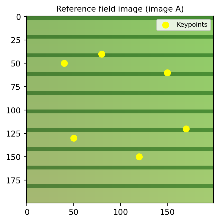
xx, yy = np.meshgrid(np.linspace(0, 1, W), np.linspace(0, 1, H))
base_r = (0.55 + 0.10 * yy).clip(0, 1)
base_g = (0.72 + 0.08 * xx).clip(0, 1)
base_b = (0.40 + 0.05 * yy).clip(0, 1)
row_mask = ((np.arange(H) % 20) < 4)[:, None]
row_mask = np.broadcast_to(row_mask, (H, W))
field_r = np.where(row_mask, base_r * 0.5, base_r)
field_g = np.where(row_mask, base_g * 0.7, base_g)
field_b = np.where(row_mask, base_b * 0.5, base_b)
img_A = np.stack([field_r, field_g, field_b], axis=2) # shape (H, W, 3)
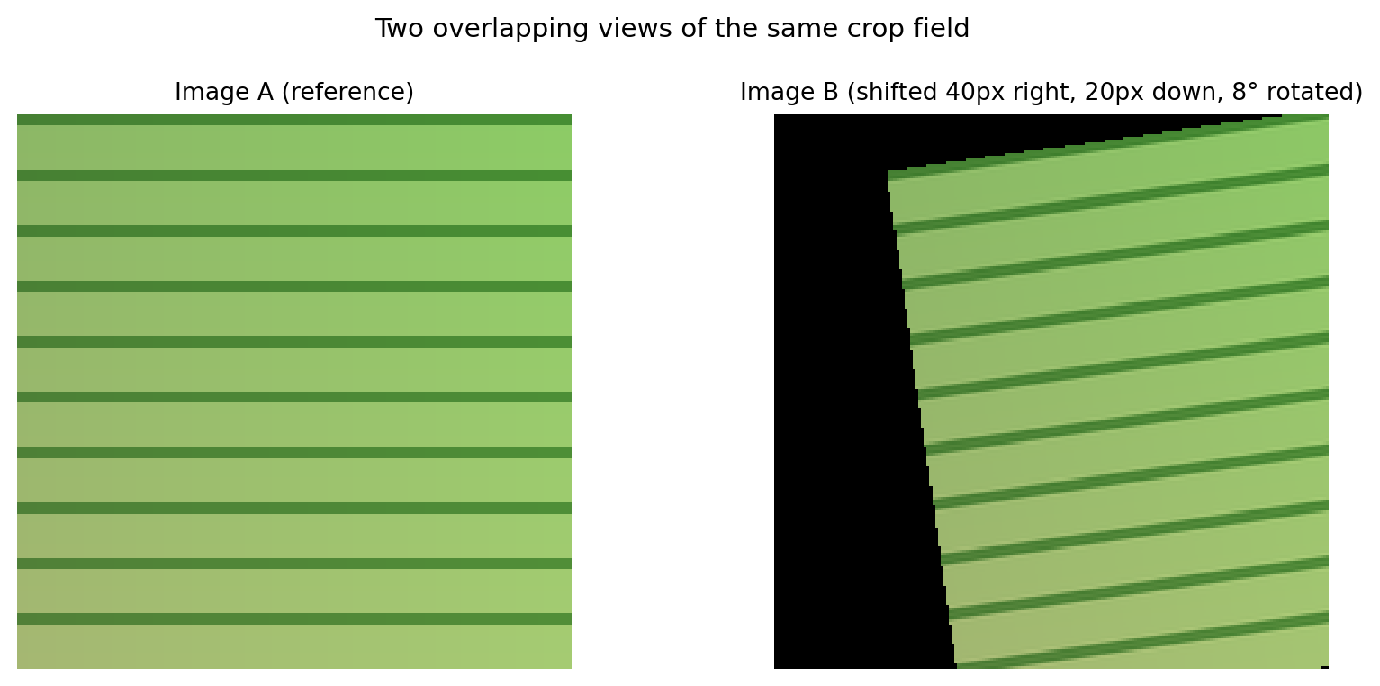
theta = np.deg2rad(8.)
c, s = np.cos(theta), np.sin(theta)
R_nd = np.array([[c, s], [-s, c]]) # shape (2, 2)
t_nd = np.array([-20.*c - 40.*s, 20.*s - 40.*c]) # shape (2,)
warped_channels = []
for ch in range(3):
w = affine_transform(img_A[:, :, ch], R_nd, offset=t_nd,
output_shape=(H, W), mode='constant', cval=0.)
warped_channels.append(w)
img_B = np.stack(warped_channels, axis=2) # shape (H, W, 3)
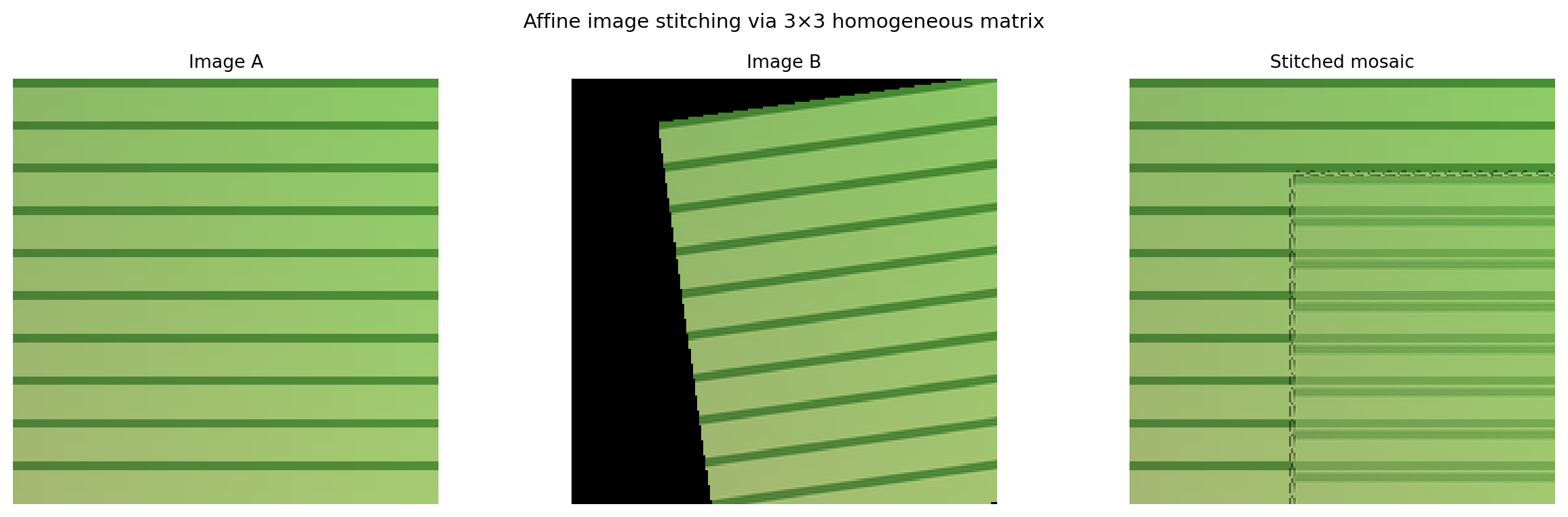
# Inverse warp: bring img_B back into img_A's frame
# M_est (A->B), so M_est_inv warps B->A
# scipy uses (row, col) — M_est is in (x=col, y=row), swap axes
# For the inverse warp of img_B onto img_A frame:
# output_pixel (r,c) in A-frame <- M_est_inv applied to (r,c)
R_inv_nd = np.array([[c, -s], [s, c]]) # shape (2, 2) — R_true (forward)
# offset: for inverse warp, offset = -R_inv * t_true (in row/col order)
t_true_rc = np.array([20., 40.]) # (row offset, col offset)
t_inv_nd = -R_inv_nd @ t_true_rc # shape (2,)
warped_B_to_A = []
for ch in range(3):
w = affine_transform(img_B[:, :, ch], R_inv_nd, offset=t_inv_nd,
output_shape=(H, W), mode='constant', cval=0.)
warped_B_to_A.append(w)
img_B_warped = np.stack(warped_B_to_A, axis=2) # shape (H, W, 3)
# Blend: where both images have signal, average; else take whichever is present
mask_A = (img_A.max(axis=2) > 0.01).astype(float) # shape (H, W)
mask_B = (img_B_warped.max(axis=2) > 0.01).astype(float) # shape (H, W)
w_A = mask_A / (mask_A + mask_B + 1e-8) # shape (H, W)
w_B = mask_B / (mask_A + mask_B + 1e-8) # shape (H, W)
mosaic = (w_A[:, :, None] * img_A
+ w_B[:, :, None] * img_B_warped).clip(0, 1) # shape (H, W, 3)
fig, axes = plt.subplots(1, 3, figsize=(13, 4))
axes[0].imshow(img_A, origin='upper'); axes[0].set_title('Image A', fontsize=10)
axes[1].imshow(img_B, origin='upper'); axes[1].set_title('Image B', fontsize=10)
axes[2].imshow(mosaic, origin='upper'); axes[2].set_title('Stitched mosaic', fontsize=10)
for ax in axes:
ax.axis('off')
fig.suptitle('Affine image stitching via 3×3 homogeneous matrix', fontsize=11)
plt.tight_layout()
plt.show()