18 Singular Value Decomposition

18.1 Geometry of the SVD: \(A = U\Sigma V^T\)

Every matrix \(A \in \mathbb{R}^{m \times n}\) can be written as a product of three structured matrices:

\[\boxed{A = U \Sigma V^T,}\]

where \(U \in \mathbb{R}^{m \times m}\) and \(V \in \mathbb{R}^{n \times n}\) are orthogonal matrices and \(\Sigma \in \mathbb{R}^{m \times n}\) is diagonal with non-negative entries. This is the singular value decomposition (SVD). Understanding it geometrically – before touching the algebra – is the single most valuable investment in this chapter.

18.1.1 The Three-Step Action of a Matrix

Apply \(A\) to a vector \(\mathbf{x} \in \mathbb{R}^n\):

\[A\mathbf{x} = U \Sigma V^T \mathbf{x}.\]

Reading right to left:

Step	Factor	Action
1	\(V^T\)	Rotate (or reflect) in the input space \(\mathbb{R}^n\)
2	\(\Sigma\)	Stretch along each coordinate axis by \(\sigma_i\)
3	\(U\)	Rotate (or reflect) in the output space \(\mathbb{R}^m\)

The phrase “every matrix is a rotate-stretch-rotate” is the core intuition. No matrix can do anything that this three-step recipe cannot.

18.1.2 The Unit Ball Becomes an Ellipsoid

The most revealing picture: apply \(A\) to the unit sphere \(S = \{\mathbf{x} : \|\mathbf{x}\|_2 = 1\} \subset \mathbb{R}^n\).

\(V^T\) rotates \(S\) – a sphere maps to a sphere, no change in shape.
\(\Sigma\) stretches: the \(i\)-th axis scales by \(\sigma_i\). The sphere becomes an ellipsoid with semi-axes \(\sigma_1 \ge \sigma_2 \ge \cdots \ge \sigma_r > 0\) (where \(r = \text{rank}(A)\); remaining axes collapse to zero).
\(U\) rotates the ellipsoid in output space.

So \(A(S)\) is an ellipsoid in \(\mathbb{R}^m\) with semi-axis lengths equal to the singular values \(\sigma_i\) and semi-axis directions equal to the columns of \(U\) (the left singular vectors).

The input directions that map to those semi-axes are the columns of \(V\) (the right singular vectors):

\[A \mathbf{v}_i = \sigma_i \mathbf{u}_i.\]

This single equation is the heart of the SVD.

18.1.3 Existence and Uniqueness

Theorem (SVD). Every \(A \in \mathbb{R}^{m \times n}\) has a singular value decomposition \(A = U\Sigma V^T\) with:

\(U \in \mathbb{R}^{m \times m}\) orthogonal (\(U^TU = UU^T = I\)),
\(V \in \mathbb{R}^{n \times n}\) orthogonal (\(V^TV = VV^T = I\)),
\(\Sigma = \text{diag}(\sigma_1, \ldots, \sigma_p)\) embedded in \(\mathbb{R}^{m \times n}\), \(p = \min(m,n)\), with \(\sigma_1 \ge \sigma_2 \ge \cdots \ge \sigma_p \ge 0\).

The singular values \(\sigma_i\) are unique. The singular vectors are unique up to sign flips (and up to rotations within repeated-singular-value subspaces).

Proof sketch. Let \(\sigma_1 = \|A\|_2 = \max_{\|\mathbf{x}\|=1}\|A\mathbf{x}\|\). A maximiser \(\mathbf{v}_1\) exists by compactness. Set \(\mathbf{u}_1 = A\mathbf{v}_1/\sigma_1\). Restricting \(A\) to the orthogonal complement of \(\mathbf{v}_1\) gives a smaller problem; induction on dimension completes the argument.

18.1.4 Thin vs. Full SVD

For \(m > n\) (tall matrix), the last \(m - n\) columns of \(U\) are never reached by \(A\). The thin (economy) SVD discards them:

\[A = \underbrace{U_r}_{m \times r} \underbrace{\Sigma_r}_{r \times r} \underbrace{V_r^T}_{r \times n}, \qquad r = \text{rank}(A).\]

In practice, np.linalg.svd(A, full_matrices=False) returns the thin form. For a rank-\(r\) matrix with \(r < \min(m,n)\), the trailing singular values are zero; truncating them gives the same product with less storage.

18.1.5 Geometric Visualization

import numpy as np
import matplotlib.pyplot as plt

rng = np.random.default_rng(181)

# Build A = U diag(3,1) V^T with explicit rotation angles
def rot2(t):
    return np.array([[np.cos(t), -np.sin(t)],   # shape (2, 2)
                     [np.sin(t),  np.cos(t)]])

theta_u = np.pi / 5
theta_v = np.pi / 7
U = rot2(theta_u)            # shape (2, 2)
V = rot2(theta_v)            # shape (2, 2)
S = np.array([3.0, 1.0])     # singular values

A = U @ np.diag(S) @ V.T     # shape (2, 2)

U_c, s_c, Vt_c = np.linalg.svd(A, full_matrices=False)
print(f"A constructed: sigma = [{S[0]:.4f}, {S[1]:.4f}]")
print(f"numpy check:   sigma = [{s_c[0]:.4f}, {s_c[1]:.4f}]")

# Unit circle and its image
angles = np.linspace(0, 2 * np.pi, 300)     # shape (300,)
circle = np.stack([np.cos(angles),
                   np.sin(angles)], axis=0)  # shape (2, 300)
ellipse = A @ circle                          # shape (2, 300)

fig, axes = plt.subplots(1, 3, figsize=(14, 5))

# Left: input space with V columns
ax = axes[0]
ax.plot(circle[0], circle[1], color='#4a90d9', lw=2)
v1 = V[:, 0]   # shape (2,)
v2 = V[:, 1]   # shape (2,)
ax.annotate('', xy=v1, xytext=[0.0, 0.0],
            arrowprops=dict(arrowstyle='->', color='#2ecc71', lw=2.5))
ax.annotate('', xy=v2, xytext=[0.0, 0.0],
            arrowprops=dict(arrowstyle='->', color='tomato', lw=2.5))
ax.text(v1[0] * 1.2, v1[1] * 1.2, r'$\mathbf{v}_1$', fontsize=13, color='#2ecc71', ha='center')
ax.text(v2[0] * 1.3, v2[1] * 1.3, r'$\mathbf{v}_2$', fontsize=13, color='tomato', ha='center')
ax.set_xlim(-1.6, 1.6)
ax.set_ylim(-1.6, 1.6)
ax.set_aspect('equal')
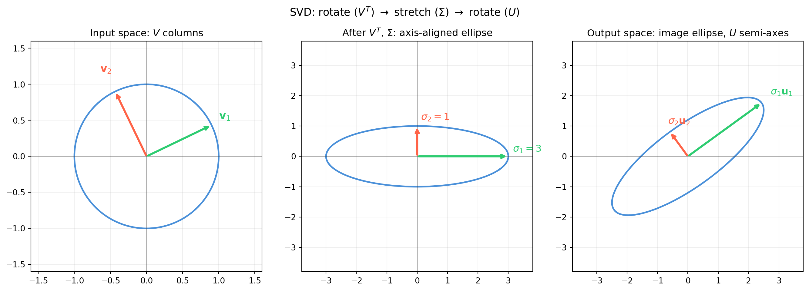
ax.set_title('Input space: $V$ columns', fontsize=12)
ax.axhline(0, color='#333333', lw=0.4, alpha=0.5)
ax.axvline(0, color='#333333', lw=0.4, alpha=0.5)
ax.grid(alpha=0.2)

# Middle: after V^T then Sigma (axis-aligned ellipse)
ax2 = axes[1]
circle_rot = V.T @ circle                    # shape (2, 300)
circle_str = np.diag(S) @ circle_rot         # shape (2, 300)
ax2.plot(circle_str[0], circle_str[1], color='#4a90d9', lw=2)
ax2.annotate('', xy=[S[0], 0.0], xytext=[0.0, 0.0],
             arrowprops=dict(arrowstyle='->', color='#2ecc71', lw=2.5))
ax2.annotate('', xy=[0.0, S[1]], xytext=[0.0, 0.0],
             arrowprops=dict(arrowstyle='->', color='tomato', lw=2.5))
ax2.text(S[0] + 0.15, 0.15, r'$\sigma_1 = 3$', fontsize=12, color='#2ecc71')
ax2.text(0.12, S[1] + 0.2, r'$\sigma_2 = 1$', fontsize=12, color='tomato')
ax2.set_xlim(-3.8, 3.8)
ax2.set_ylim(-3.8, 3.8)
ax2.set_aspect('equal')
ax2.set_title(r'After $V^T$, $\Sigma$: axis-aligned ellipse', fontsize=12)
ax2.axhline(0, color='#333333', lw=0.4, alpha=0.5)
ax2.axvline(0, color='#333333', lw=0.4, alpha=0.5)
ax2.grid(alpha=0.2)

# Right: output space with U columns and final ellipse
ax3 = axes[2]
ax3.plot(ellipse[0], ellipse[1], color='#4a90d9', lw=2)
u1 = U[:, 0]   # shape (2,)
u2 = U[:, 1]   # shape (2,)
ax3.annotate('', xy=u1 * S[0], xytext=[0.0, 0.0],
             arrowprops=dict(arrowstyle='->', color='#2ecc71', lw=2.5))
ax3.annotate('', xy=u2 * S[1], xytext=[0.0, 0.0],
             arrowprops=dict(arrowstyle='->', color='tomato', lw=2.5))
ax3.text(u1[0] * S[0] * 1.1 + 0.05, u1[1] * S[0] * 1.1 + 0.1,
         r'$\sigma_1 \mathbf{u}_1$', fontsize=12, color='#2ecc71')
ax3.text(u2[0] * S[1] * 1.2 + 0.05, u2[1] * S[1] * 1.2 + 0.1,
         r'$\sigma_2 \mathbf{u}_2$', fontsize=12, color='tomato')
ax3.set_xlim(-3.8, 3.8)
ax3.set_ylim(-3.8, 3.8)
ax3.set_aspect('equal')
ax3.set_title(r'Output space: image ellipse, $U$ semi-axes', fontsize=12)
ax3.axhline(0, color='#333333', lw=0.4, alpha=0.5)
ax3.axvline(0, color='#333333', lw=0.4, alpha=0.5)
ax3.grid(alpha=0.2)

fig.suptitle(r'SVD: rotate ($V^T$) $\to$ stretch ($\Sigma$) $\to$ rotate ($U$)', fontsize=13)
fig.tight_layout()
plt.savefig('ch18-svd/fig-svd-geometry.png', dpi=150, bbox_inches='tight')
plt.show()

A constructed: sigma = [3.0000, 1.0000]
numpy check:   sigma = [3.0000, 1.0000]

18.1.6 Relation to Eigendecomposition

The SVD and eigendecomposition are connected but distinct.

\[A^TA = (V\Sigma^T U^T)(U\Sigma V^T) = V(\Sigma^T\Sigma)V^T,\]

so the columns of \(V\) are eigenvectors of \(A^TA\) and \(\sigma_i^2 = \lambda_i(A^TA)\). Similarly \(AA^T = U\Sigma\Sigma^TU^T\), so columns of \(U\) are eigenvectors of \(AA^T\).

Key differences:

	Eigendecomposition	SVD
Matrix shape	Square only	Any \(m \times n\)
Existence (real)	Not guaranteed	Always exists
Factors	May be complex	\(U\), \(V\) always real orthogonal
Diagonal entries	Can be negative	\(\sigma_i \ge 0\)

The SVD is the universally applicable factorization; eigendecomposition is the special case for symmetric positive semidefinite matrices, where \(U = V\).

18.1.7 Rank and the Four Fundamental Subspaces

Let \(r = \text{rank}(A)\). The SVD directly reveals all four subspaces:

Subspace	Basis
\(\text{Col}(A)\)	\(\mathbf{u}_1, \ldots, \mathbf{u}_r\) (first \(r\) columns of \(U\))
\(\text{Null}(A^T)\)	\(\mathbf{u}_{r+1}, \ldots, \mathbf{u}_m\) (last \(m-r\) columns of \(U\))
\(\text{Row}(A)\)	\(\mathbf{v}_1, \ldots, \mathbf{v}_r\) (first \(r\) columns of \(V\))
\(\text{Null}(A)\)	\(\mathbf{v}_{r+1}, \ldots, \mathbf{v}_n\) (last \(n-r\) columns of \(V\))

This is one reason the SVD is the most informative factorization: it simultaneously diagonalises \(A\) and reads off all four subspaces.

18.1.8 Numerical Example

import numpy as np

A = np.array([[1.0, 2.0],   # shape (3, 2)
              [3.0, 4.0],
              [5.0, 6.0]])

U, s, Vt = np.linalg.svd(A, full_matrices=False)
# U shape (3, 2), s shape (2,), Vt shape (2, 2)  -- thin SVD

print(f"Singular values: sigma_1 = {s[0]:.6f}, sigma_2 = {s[1]:.6f}")
print(f"\nU (shape {U.shape}):")
print(U.round(6))
print(f"\nV^T (shape {Vt.shape}):")
print(Vt.round(6))

A_rec = U @ np.diag(s) @ Vt             # shape (3, 2)
print(f"\n||A - U Sigma V^T||_F = {np.linalg.norm(A - A_rec):.2e}  (reconstruction)")

print(f"U^T U = I? max|U^TU - I| = {np.abs(U.T @ U - np.eye(2)).max():.2e}")

# Sigma_i^2 vs eigenvalues of A^T A
evals = np.sort(np.linalg.eigvalsh(A.T @ A))[::-1]  # shape (2,)
print(f"\nsigma^2 vs lambda(A^T A):")
for i in range(2):
    print(f"  sigma_{i+1}^2 = {s[i]**2:.6f},  lambda_{i+1} = {evals[i]:.6f}")

Singular values: sigma_1 = 9.525518, sigma_2 = 0.514301

U (shape (3, 2)):
[[-0.229848  0.883461]
 [-0.524745  0.240782]
 [-0.819642 -0.401896]]

V^T (shape (2, 2)):
[[-0.619629 -0.784894]
 [-0.784894  0.619629]]

||A - U Sigma V^T||_F = 1.39e-15  (reconstruction)
U^T U = I? max|U^TU - I| = 2.22e-16

sigma^2 vs lambda(A^T A):
  sigma_1^2 = 90.735495,  lambda_1 = 90.735495
  sigma_2^2 = 0.264505,  lambda_2 = 0.264505

18.1.9 Exercises

18.1.1 Let \(A = \begin{bmatrix}4 & 0 \\ 0 & 3\end{bmatrix}\). Write down the SVD by inspection. What are \(U\), \(\Sigma\), \(V^T\)? What ellipse does \(A\) map the unit circle to?

18.1.2 Let \(A = \begin{bmatrix}0 & 1 \\ 1 & 0\end{bmatrix}\) (permutation). Show that \(A^TA = I\), so all singular values equal 1. Identify \(U\), \(\Sigma\), \(V^T\).

18.1.3 Prove that \(\|A\|_F^2 = \sum_i \sigma_i^2\). (Hint: \(\|A\|_F^2 = \text{tr}(A^TA)\) and the trace is the sum of eigenvalues.)

18.1.4 If \(A \in \mathbb{R}^{m \times n}\) has rank \(r\), show that \(A = \sum_{i=1}^r \sigma_i \mathbf{u}_i \mathbf{v}_i^T\) (outer product form of the SVD). Why does the sum stop at \(r\)?

18.2 Singular Values and Their Meaning

Singular values are not just algebraic by-products of the SVD – they are the intrinsic geometry of a linear map, independent of the choice of basis in input or output space. Each \(\sigma_i\) measures how much \(A\) stretches in one direction; together they encode the rank, the norms, the condition number, and the low-rank structure of \(A\).

18.2.1 Singular Values as Stretch Factors

From §18.1, applying \(A\) to the unit sphere produces an ellipsoid with semi-axis lengths \(\sigma_1 \ge \sigma_2 \ge \cdots \ge \sigma_r > 0 = \sigma_{r+1} = \cdots = \sigma_p\), where \(r = \text{rank}(A)\) and \(p = \min(m,n)\).

The maximum stretch factor is \(\sigma_1\): \[\sigma_1 = \|A\|_2 = \max_{\|\mathbf{x}\|_2 = 1} \|A\mathbf{x}\|_2.\]

The minimum non-zero stretch factor is \(\sigma_r\) (equivalently \(\sigma_{\min}\) when \(A\) is square and invertible): \[\sigma_{\min} = \min_{\|\mathbf{x}\|_2 = 1} \|A\mathbf{x}\|_2 \qquad (\text{for full-rank } A).\]

A small \(\sigma_{\min}\) means \(A\) nearly collapses space in some direction – the matrix is close to singular.

18.2.2 Rank via Singular Values

\[\text{rank}(A) = \text{number of non-zero singular values}.\]

Numerically, singular values computed by floating-point algorithms are never exactly zero. The numerical rank uses a threshold: \[\text{rank}_\varepsilon(A) = \#\{i : \sigma_i > \varepsilon\}.\]

A common choice is \(\varepsilon = \sigma_1 \cdot \max(m,n) \cdot \epsilon_{\text{machine}}\) (the default rcond in numpy.linalg.lstsq). Values below this threshold are considered numerically zero.

18.2.3 Matrix Norms Expressed via Singular Values

All three standard matrix norms have clean SVD expressions:

Norm	Definition	SVD expression
Spectral (operator) \(\\|A\\|_2\)	\(\max_{\\|\mathbf{x}\\|=1}\\|A\mathbf{x}\\|\)	\(\sigma_1\)
Frobenius \(\\|A\\|_F\)	\(\sqrt{\sum_{i,j} a_{ij}^2}\)	\(\sqrt{\sigma_1^2 + \cdots + \sigma_p^2}\)
Nuclear \(\\|A\\|_*\)	sum of singular values	\(\sigma_1 + \cdots + \sigma_p\)

The Frobenius norm identity follows from \(\|A\|_F^2 = \text{tr}(A^TA) = \sum_i \lambda_i(A^TA) = \sum_i \sigma_i^2\).

The nuclear norm is the convex relaxation of rank – minimising \(\|A\|_*\) promotes low-rank solutions (used in matrix completion, collaborative filtering).

18.2.4 Condition Number

For a square invertible matrix \(A\): \[\kappa(A) = \|A\|_2 \|A^{-1}\|_2 = \frac{\sigma_1}{\sigma_n}.\]

The condition number measures how much a relative perturbation in \(\mathbf{b}\) gets amplified when solving \(A\mathbf{x} = \mathbf{b}\): \[\frac{\|\delta \mathbf{x}\|}{\|\mathbf{x}\|} \le \kappa(A) \frac{\|\delta \mathbf{b}\|}{\|\mathbf{b}\|}.\]

Rules of thumb: \(\kappa \approx 10^k\) means roughly \(k\) decimal digits are lost to round-off. \(\kappa > 1/\epsilon_{\text{machine}}\) (\(\approx 10^{16}\) for double) means the matrix is numerically singular.

Determinant and singular values (square \(n \times n\)): \[|\det(A)| = \prod_{i=1}^n \sigma_i.\]

So \(\det(A) = 0 \iff\) at least one \(\sigma_i = 0 \iff A\) is singular.

18.2.5 Singular Value Decay and Low-Rank Structure

The rate at which singular values decay reveals whether a matrix has latent low-rank structure:

Flat spectrum (\(\sigma_i \approx \sigma_j\) for all \(i,j\)): no low-rank structure; full-rank information. Example: random Gaussian matrices.
Fast decay: the matrix is well-approximated by a low-rank matrix. Example: covariance matrices of smooth processes, document-term matrices with topic structure.
Step drop (\(\sigma_k \gg \sigma_{k+1} \approx \cdots \approx 0\)): matrix is numerically rank-\(k\).

import numpy as np
import matplotlib.pyplot as plt

rng = np.random.default_rng(182)

# Three matrices: random full-rank, low-rank + noise, near-rank-deficient
n = 50

# Full-rank random
A_rand = rng.standard_normal((n, n))      # shape (50, 50)
s_rand = np.linalg.svd(A_rand, compute_uv=False)  # shape (50,)

# Low-rank: rank-5 signal + small noise
U5 = rng.standard_normal((n, 5))          # shape (50, 5)
V5 = rng.standard_normal((n, 5))          # shape (50, 5)
A_lr = U5 @ V5.T + 0.1 * rng.standard_normal((n, n))  # shape (50, 50)
s_lr = np.linalg.svd(A_lr, compute_uv=False)           # shape (50,)

# Near-rank-deficient: exponential decay
sigma_exp = np.exp(-np.arange(n) / 5.0)   # shape (50,)
A_exp = (rng.standard_normal((n, n)) * sigma_exp).T    # shape (50, 50)
s_exp = np.linalg.svd(A_exp, compute_uv=False)         # shape (50,)

fig, axes = plt.subplots(1, 2, figsize=(13, 5))

ax = axes[0]
ax.plot(s_rand / s_rand[0], color='#4a90d9', lw=2, label='random (flat)')
ax.plot(s_lr   / s_lr[0],   color='#2ecc71', lw=2, label='low-rank + noise (step drop)')
ax.plot(s_exp  / s_exp[0],  color='tomato',  lw=2, label='exponential decay')
ax.set_xlabel('Index $i$', fontsize=11)
ax.set_ylabel('$\\sigma_i / \\sigma_1$', fontsize=11)
ax.set_title('Singular value spectra (normalised)', fontsize=12)
ax.legend(fontsize=10)
ax.grid(alpha=0.2)

ax2 = axes[1]
ax2.semilogy(s_rand / s_rand[0], color='#4a90d9', lw=2, label='random')
ax2.semilogy(s_lr   / s_lr[0],   color='#2ecc71', lw=2, label='low-rank + noise')
ax2.semilogy(s_exp  / s_exp[0],  color='tomato',  lw=2, label='exp decay')
ax2.set_xlabel('Index $i$', fontsize=11)
ax2.set_ylabel('$\\sigma_i / \\sigma_1$ (log scale)', fontsize=11)
ax2.set_title('Singular value spectra (log scale)', fontsize=12)
ax2.legend(fontsize=10)
ax2.grid(alpha=0.2)

fig.tight_layout()
plt.savefig('ch18-svd/fig-svd-spectra.png', dpi=150, bbox_inches='tight')
plt.show()

print("=== Spectral properties ===")
for name, A, s in [("random", A_rand, s_rand),
                   ("low-rank+noise", A_lr, s_lr),
                   ("exp-decay", A_exp, s_exp)]:
    kappa = s[0] / s[-1]
    rank_eps = np.sum(s > s[0] * n * np.finfo(float).eps)
    print(f"\n{name}:")
    print(f"  ||A||_2  = {s[0]:.3f}")
    print(f"  ||A||_F  = {np.sqrt(np.sum(s**2)):.3f}")
    print(f"  ||A||_*  = {np.sum(s):.3f}")
    print(f"  kappa    = {kappa:.2e}")
    print(f"  num rank = {rank_eps}")

=== Spectral properties ===

random:
  ||A||_2  = 13.844
  ||A||_F  = 49.858
  ||A||_*  = 298.044
  kappa    = 5.39e+01
  num rank = 50

low-rank+noise:
  ||A||_2  = 70.760
  ||A||_F  = 114.940
  ||A||_*  = 273.275
  kappa    = 2.63e+04
  num rank = 50

exp-decay:
  ||A||_2  = 7.220
  ||A||_F  = 11.996
  ||A||_*  = 35.909
  kappa    = 1.38e+05
  num rank = 50

18.2.6 Singular Values of Common Matrices

Matrix type	Singular values
Orthogonal \(Q\)	All \(\sigma_i = 1\)
Diagonal \(D\)	\(\sigma_i = \|d_i\|\)
Scalar multiple \(\alpha A\)	\(\|\alpha\| \sigma_i(A)\)
\(A^T\)	Same as \(\sigma_i(A)\)
\(AB\)	\(\sigma_i(AB) \le \sigma_1(A)\sigma_i(B)\) (submultiplicativity)

The identity \(\sigma_i(A^T) = \sigma_i(A)\) follows because \(A^TA\) and \(AA^T\) share non-zero eigenvalues.

18.2.7 Exercises

18.2.1 A matrix \(A \in \mathbb{R}^{3 \times 3}\) has singular values 5, 3, 0.1. Compute \(\|A\|_2\), \(\|A\|_F\), \(\|A\|_*\), \(\kappa(A)\), and \(|\det(A)|\).

18.2.2 Show that for any orthogonal matrix \(Q \in \mathbb{R}^{n \times n}\), all singular values equal 1. Conclude that \(\|QA\|_2 = \|A\|_2\) and \(\|QA\|_F = \|A\|_F\) for any \(A\).

18.2.3 A sensor fusion matrix has condition number \(\kappa \approx 10^{12}\). If we solve \(A\mathbf{x} = \mathbf{b}\) in double precision (\(\epsilon \approx 10^{-16}\)), roughly how many digits of the answer can we trust?

18.2.4 Let \(A = \mathbf{u}\mathbf{v}^T\) (rank-1 outer product) with \(\|\mathbf{u}\| = \|\mathbf{v}\| = 1\). What are the singular values of \(A\)? Identify \(U\), \(\Sigma\), \(V^T\) explicitly.

18.3 Low-Rank Approximation: Eckart-Young Theorem

The outer-product form of the SVD,

\[A = \sum_{i=1}^r \sigma_i \mathbf{u}_i \mathbf{v}_i^T,\]

decomposes \(A\) into \(r\) rank-1 layers, each of magnitude \(\sigma_i\). Truncating this sum at \(k < r\) terms gives the best possible rank-\(k\) approximation – not just among SVD-based approximations, but among all rank-\(k\) matrices. This is the Eckart-Young theorem.

18.3.1 Statement and Proof

Theorem (Eckart-Young, 1936). Let \(A = U\Sigma V^T\) with singular values \(\sigma_1 \ge \cdots \ge \sigma_r > 0\). Define the truncated SVD:

\[A_k = \sum_{i=1}^k \sigma_i \mathbf{u}_i \mathbf{v}_i^T = U_k \Sigma_k V_k^T,\]

where \(U_k\) and \(V_k\) hold the first \(k\) columns of \(U\) and \(V\), and \(\Sigma_k = \text{diag}(\sigma_1, \ldots, \sigma_k)\). Then:

\[\|A - A_k\|_2 = \sigma_{k+1}, \qquad \|A - A_k\|_F = \sqrt{\sigma_{k+1}^2 + \cdots + \sigma_r^2},\]

and for any matrix \(B\) with \(\text{rank}(B) \le k\):

\[\|A - A_k\|_2 \le \|A - B\|_2, \qquad \|A - A_k\|_F \le \|A - B\|_F.\]

Proof sketch (spectral norm). We need to show no rank-\(k\) matrix \(B\) satisfies \(\|A - B\|_2 < \sigma_{k+1}\). Suppose \(\text{rank}(B) \le k\). Then \(\text{Null}(B)\) has dimension at least \(n - k\). The subspace \(\text{span}\{\mathbf{v}_1, \ldots, \mathbf{v}_{k+1}\}\) has dimension \(k+1\), so by dimension counting it intersects \(\text{Null}(B)\) in a vector \(\mathbf{x}\) with \(\|\mathbf{x}\| = 1\). Then: \[\|(A - B)\mathbf{x}\|_2 = \|A\mathbf{x}\|_2 \ge \sigma_{k+1}.\] The Frobenius case follows similarly by choosing the best subspace.

18.3.2 Interpretation

The approximation error in the Frobenius norm is the tail energy: \[\frac{\|A - A_k\|_F^2}{\|A\|_F^2} = \frac{\sigma_{k+1}^2 + \cdots + \sigma_r^2}{\sigma_1^2 + \cdots + \sigma_r^2}.\]

This motivates the explained variance ratio (borrowed from PCA): \[\text{EVR}(k) = \frac{\sum_{i=1}^k \sigma_i^2}{\sum_{i=1}^r \sigma_i^2}.\]

Choosing \(k\) so that \(\text{EVR}(k) \ge 0.99\) (99% of Frobenius energy) is a common heuristic for dimension reduction.

18.3.3 Image Compression via Truncated SVD

A grayscale image is a matrix \(A \in \mathbb{R}^{m \times n}\). The truncated SVD at rank \(k\) requires storing \(k(m + n + 1)\) numbers instead of \(mn\), a compression ratio of \(k(m + n + 1) / (mn)\).

import numpy as np
import matplotlib.pyplot as plt

rng = np.random.default_rng(183)

# Synthesise a structured grayscale image (smooth + edge features)
m, n = 128, 128
x = np.linspace(0, 1, n)    # shape (128,)
y = np.linspace(0, 1, m)    # shape (128,)
X, Y = np.meshgrid(x, y)    # X, Y each shape (128, 128)

# Combine smooth gradient, radial basis, and step edge
img = (0.4 * np.sin(4 * np.pi * X) * np.cos(3 * np.pi * Y)
       + 0.3 * np.exp(-((X - 0.5)**2 + (Y - 0.5)**2) / 0.05)
       + 0.2 * (X > 0.6).astype(float)
       + 0.05 * rng.standard_normal((m, n)))  # shape (128, 128)
img = (img - img.min()) / (img.max() - img.min())  # scale to [0, 1]

U, s, Vt = np.linalg.svd(img, full_matrices=False)  # U (128,128), s (128,), Vt (128,128)

ranks = [1, 5, 15, 40]
fig, axes = plt.subplots(1, len(ranks) + 1, figsize=(15, 3.5))

ax0 = axes[0]
ax0.imshow(img, cmap='gray', vmin=0, vmax=1)
ax0.set_title('Original', fontsize=11)
ax0.axis('off')

for ax, k in zip(axes[1:], ranks):
    img_k = U[:, :k] @ np.diag(s[:k]) @ Vt[:k, :]   # shape (128, 128)
    img_k = np.clip(img_k, 0, 1)
    rel_err = np.linalg.norm(img - img_k, 'fro') / np.linalg.norm(img, 'fro')
    ratio = k * (m + n + 1) / (m * n)
    ax.imshow(img_k, cmap='gray', vmin=0, vmax=1)
    ax.set_title(f'rank {k}\nerr={rel_err:.3f}, ratio={ratio:.2f}', fontsize=10)
    ax.axis('off')

fig.suptitle('Truncated SVD image compression', fontsize=12)
fig.tight_layout()
plt.savefig('ch18-svd/fig-svd-compression.png', dpi=150, bbox_inches='tight')
plt.show()

18.3.4 Explained Variance and Choosing Rank

import numpy as np
import matplotlib.pyplot as plt

rng = np.random.default_rng(1831)

# Recompute SVD of the same structured image
m, n = 128, 128
x = np.linspace(0, 1, n)
y = np.linspace(0, 1, m)
X, Y = np.meshgrid(x, y)
img = (0.4 * np.sin(4 * np.pi * X) * np.cos(3 * np.pi * Y)
       + 0.3 * np.exp(-((X - 0.5)**2 + (Y - 0.5)**2) / 0.05)
       + 0.2 * (X > 0.6).astype(float)
       + 0.05 * rng.standard_normal((m, n)))

s = np.linalg.svd(img, compute_uv=False)  # shape (128,)

energy = np.cumsum(s**2) / np.sum(s**2)          # shape (128,)  -- cumulative explained variance
k_90 = np.searchsorted(energy, 0.90) + 1
k_99 = np.searchsorted(energy, 0.99) + 1

fig, axes = plt.subplots(1, 2, figsize=(12, 4.5))

ax = axes[0]
ax.semilogy(s, color='#4a90d9', lw=2)
ax.set_xlabel('Rank $i$', fontsize=11)
ax.set_ylabel('$\\sigma_i$ (log scale)', fontsize=11)
ax.set_title('Singular value spectrum', fontsize=12)
ax.grid(alpha=0.2)

ax2 = axes[1]
ax2.plot(energy, color='#4a90d9', lw=2)
ax2.axhline(0.90, color='#2ecc71', lw=1.5, linestyle='--',
            label=f'90% at k={k_90}')
ax2.axhline(0.99, color='tomato', lw=1.5, linestyle='--',
            label=f'99% at k={k_99}')
ax2.axvline(k_90, color='#2ecc71', lw=1, linestyle=':')
ax2.axvline(k_99, color='tomato', lw=1, linestyle=':')
ax2.set_xlabel('Rank $k$', fontsize=11)
ax2.set_ylabel('Cumulative explained variance', fontsize=11)
ax2.set_title('Explained variance ratio', fontsize=12)
ax2.legend(fontsize=10)
ax2.grid(alpha=0.2)

fig.tight_layout()
plt.savefig('ch18-svd/fig-svd-evr.png', dpi=150, bbox_inches='tight')
plt.show()

print(f"Singular values: sigma_1 = {s[0]:.4f}, sigma_2 = {s[1]:.4f}, sigma_5 = {s[4]:.4f}")
print(f"90% energy at rank {k_90}  (compression ratio {k_90*(m+n+1)/(m*n):.3f})")
print(f"99% energy at rank {k_99}  (compression ratio {k_99*(m+n+1)/(m*n):.3f})")

Singular values: sigma_1 = 25.8687, sigma_2 = 20.4100, sigma_5 = 1.0814
90% energy at rank 2  (compression ratio 0.031)
99% energy at rank 42  (compression ratio 0.659)

18.3.5 Low-Rank Approximation Error

import numpy as np

rng = np.random.default_rng(1832)

# Verify Eckart-Young bounds on a random matrix
m, n = 40, 30
A = rng.standard_normal((m, n))          # shape (40, 30)
U, s, Vt = np.linalg.svd(A, full_matrices=False)
# U shape (40, 30), s shape (30,), Vt shape (30, 30)

print("Eckart-Young verification:")
print(f"{'k':>4}  {'||A-Ak||_2':>12}  {'sigma_k+1':>12}  {'||A-Ak||_F':>12}  {'tail_energy':>12}")
for k in [1, 3, 5, 10, 20]:
    Ak = U[:, :k] @ np.diag(s[:k]) @ Vt[:k, :]    # shape (40, 30)
    err2 = np.linalg.norm(A - Ak, 2)
    errF = np.linalg.norm(A - Ak, 'fro')
    tail = np.sqrt(np.sum(s[k:]**2))
    sig_next = s[k] if k < len(s) else 0.0
    print(f"{k:>4}  {err2:>12.6f}  {sig_next:>12.6f}  {errF:>12.6f}  {tail:>12.6f}")

Eckart-Young verification:
   k    ||A-Ak||_2     sigma_k+1    ||A-Ak||_F   tail_energy
   1     10.480380     10.480380     32.941367     32.941367
   3      9.413556      9.413556     29.614517     29.614517
   5      8.543903      8.543903     26.659923     26.659923
  10      6.763732      6.763732     19.739363     19.739363
  20      3.662936      3.662936      8.458684      8.458684

18.3.6 Applications

Low-rank approximation appears throughout ML and signal processing:

Principal Component Analysis (PCA): Center the data matrix \(X\); the top-\(k\) singular vectors of \(X\) (equivalently eigenvectors of the covariance matrix) define the principal subspace. The truncated SVD computes PCA directly.

Latent Semantic Analysis: Documents are represented as term-frequency vectors; the low-rank SVD reveals latent topics.

Collaborative filtering / recommender systems: The user-item rating matrix is sparse and approximately low-rank; matrix factorization (closely related to SVD) fills in missing entries.

Signal denoising: If a signal matrix has a low-rank true component plus noise, the truncated SVD separates them.

18.3.7 Exercises

18.3.1 Let \(A = \mathbf{u}\mathbf{v}^T\) (rank-1) with \(\|\mathbf{u}\| = \|\mathbf{v}\| = 1\). What is \(A_k\) for \(k \ge 1\)? What is \(\|A - A_1\|_2\)?

18.3.2 A \(200 \times 300\) matrix \(A\) has Frobenius norm 50 and \(\sigma_1 = 30\). What is \(\|A - A_1\|_F\)? How much of the Frobenius energy does rank-1 capture?

18.3.3 Show that \(\|A - A_k\|_F^2 = \|A\|_F^2 - \|A_k\|_F^2\). (Hint: Use the outer-product form and orthonormality of \(\mathbf{u}_i\), \(\mathbf{v}_i\).)

18.3.4 A GPS trajectory covariance matrix (size \(100 \times 100\)) has singular values decaying like \(\sigma_i \approx e^{-i/10}\). At what rank \(k\) does the truncated SVD capture 99% of the Frobenius energy? Write a short computation.

18.4 Kabsch Algorithm: Optimal Rotation Between Point Sets

Given two sets of corresponding 3-D points \(\{P_i\}\) and \(\{Q_i\}\), the Kabsch algorithm finds the rotation (and translation) that best aligns them in the least-squares sense. It is the foundational step in point cloud registration, protein structure comparison, and hand-eye calibration.

18.4.1 Problem Formulation

Given \(m\) corresponding point pairs \(\mathbf{p}_i, \mathbf{q}_i \in \mathbb{R}^3\), find the rotation \(R \in \text{SO}(3)\) and translation \(\mathbf{t} \in \mathbb{R}^3\) minimising:

\[\min_{R \in \text{SO}(3),\, \mathbf{t}} \sum_{i=1}^m \|\mathbf{q}_i - (R\mathbf{p}_i + \mathbf{t})\|_2^2.\]

Step 1 – Remove translation. The optimal translation is determined by the centroids regardless of \(R\):

\[\hat{\mathbf{t}} = \bar{\mathbf{q}} - R\bar{\mathbf{p}}, \qquad \bar{\mathbf{p}} = \frac{1}{m}\sum_i \mathbf{p}_i, \quad \bar{\mathbf{q}} = \frac{1}{m}\sum_i \mathbf{q}_i.\]

Substituting and centring, the problem reduces to finding \(R\) that minimises \(\sum_i \|\tilde{\mathbf{q}}_i - R\tilde{\mathbf{p}}_i\|_2^2\) where \(\tilde{\mathbf{p}}_i = \mathbf{p}_i - \bar{\mathbf{p}}\) and \(\tilde{\mathbf{q}}_i = \mathbf{q}_i - \bar{\mathbf{q}}\).

Step 2 – Reduce to maximising a trace. Expanding: \[\sum_i \|\tilde{\mathbf{q}}_i - R\tilde{\mathbf{p}}_i\|^2 = \sum_i \|\tilde{\mathbf{q}}_i\|^2 + \sum_i \|R\tilde{\mathbf{p}}_i\|^2 - 2 \sum_i \tilde{\mathbf{q}}_i^T R \tilde{\mathbf{p}}_i.\]

Since \(\|R\mathbf{p}\| = \|\mathbf{p}\|\) (rotation preserves norms), the first two terms are constants. We need to maximise \(\text{tr}(R^T H)\) where:

\[H = \sum_{i=1}^m \tilde{\mathbf{p}}_i \tilde{\mathbf{q}}_i^T = \tilde{P}^T \tilde{Q} \in \mathbb{R}^{3 \times 3},\]

with \(\tilde{P}, \tilde{Q} \in \mathbb{R}^{m \times 3}\) the centred point matrices.

18.4.2 SVD Solution and Determinant Correction

Step 3 – SVD of the cross-covariance matrix. Compute \(H = U \Sigma V^T\).

For any orthogonal \(R\) and positive semidefinite \(\Sigma\): \[\text{tr}(R^T H) = \text{tr}(R^T U \Sigma V^T) = \text{tr}(V^T R^T U \Sigma).\]

Let \(M = V^T R^T U\) – also orthogonal. Then \(\text{tr}(M\Sigma) \le \sum_i \sigma_i\) (trace of orthogonal times diagonal PSD is maximised when \(M = I\)), achieved by \(M = I\), i.e., \(R = UV^T\).

Step 4 – Reflection check. If \(\det(UV^T) = -1\), then \(R = UV^T\) is a reflection, not a rotation. This happens when \(H\) is rank-deficient or the point sets are nearly coplanar. The correction uses the closest rotation:

\[\boxed{R^* = V \begin{pmatrix}1 & & \\ & 1 & \\ & & d\end{pmatrix} U^T, \qquad d = \det(V U^T) \in \{+1, -1\}.}\]

Setting \(d = \text{sign}(\det(VU^T))\) ensures \(\det(R^*) = +1\).

Full algorithm:

Centre both point sets: \(\tilde{P}\), \(\tilde{Q}\).
Compute cross-covariance: \(H = \tilde{P}^T \tilde{Q}\).
SVD: \(H = U\Sigma V^T\).
Compute \(d = \text{sign}(\det(V U^T))\).
\(R^* = V \,\text{diag}(1, 1, d)\, U^T\).
\(\mathbf{t}^* = \bar{\mathbf{q}} - R^* \bar{\mathbf{p}}\).

18.4.3 Root-Mean-Square Deviation

The quality of alignment is measured by the RMSD: \[\text{RMSD} = \sqrt{\frac{1}{m} \sum_{i=1}^m \|\mathbf{q}_i - (R^*\mathbf{p}_i + \mathbf{t}^*)\|_2^2}.\]

After applying the optimal \(R^*\) and \(\mathbf{t}^*\), the minimum achievable RMSD is: \[\text{RMSD}_{\min}^2 = \frac{1}{m}\left(\sum_i \|\tilde{\mathbf{q}}_i\|^2 + \sum_i \|\tilde{\mathbf{p}}_i\|^2 - 2\sum_{i=1}^k \sigma_i\right).\]

18.4.4 Implementation and Demonstration

import numpy as np
import matplotlib.pyplot as plt

rng = np.random.default_rng(184)

def kabsch(P, Q):
    """
    Kabsch algorithm: find R in SO(3) and t minimising sum ||q_i - (R p_i + t)||^2.
    P, Q: shape (m, 3) -- corresponding point sets.
    Returns R (3, 3), t (3,), rmsd (scalar).
    """
    # Centre
    p_bar = P.mean(axis=0)   # shape (3,)
    q_bar = Q.mean(axis=0)   # shape (3,)
    P_c = P - p_bar           # shape (m, 3)
    Q_c = Q - q_bar           # shape (m, 3)

    # Cross-covariance matrix
    H = P_c.T @ Q_c           # shape (3, 3)

    # SVD
    U, s, Vt = np.linalg.svd(H)    # U (3,3), s (3,), Vt (3,3)
    V = Vt.T                         # shape (3, 3)

    # Determinant correction: avoid reflection
    d = np.sign(np.linalg.det(V @ U.T))     # scalar in {+1, -1}
    D = np.diag(np.array([1.0, 1.0, d]))    # shape (3, 3)
    R = V @ D @ U.T                          # shape (3, 3)

    # Translation
    t = q_bar - R @ p_bar           # shape (3,)

    # RMSD
    Q_fit = (R @ P.T).T + t         # shape (m, 3)
    rmsd = np.sqrt(np.mean(np.sum((Q - Q_fit)**2, axis=1)))

    return R, t, rmsd

# Ground truth transform: rotation by 40 degrees around a tilted axis + translation
angle = np.radians(40)
axis = np.array([1.0, 1.0, 0.5])
axis = axis / np.linalg.norm(axis)    # shape (3,)  -- unit rotation axis
c, s_a = np.cos(angle), np.sin(angle)
K = np.array([[0, -axis[2], axis[1]],   # shape (3, 3) -- skew symmetric
              [axis[2], 0, -axis[0]],
              [-axis[1], axis[0], 0]])
R_true = c * np.eye(3) + (1 - c) * np.outer(axis, axis) + s_a * K  # shape (3, 3)
t_true = np.array([0.5, -0.3, 0.8])    # shape (3,)

# Random point cloud
m = 50
P = rng.standard_normal((m, 3))        # shape (50, 3)
Q_clean = (R_true @ P.T).T + t_true   # shape (50, 3)  -- exact transform
noise = 0.02 * rng.standard_normal((m, 3))  # shape (50, 3)
Q = Q_clean + noise                    # shape (50, 3)  -- with noise

R_est, t_est, rmsd = kabsch(P, Q)

print("=== Kabsch registration ===")
print(f"RMSD after alignment: {rmsd:.4f}  (noise level ~{0.02:.4f})")
print(f"\nRotation error ||R_est - R_true||_F = {np.linalg.norm(R_est - R_true):.2e}")
print(f"Translation error ||t_est - t_true||  = {np.linalg.norm(t_est - t_true):.2e}")
print(f"\ndet(R_est) = {np.linalg.det(R_est):.6f}  (should be +1)")
print(f"R_est orthogonal: max|R^TR - I| = {np.abs(R_est.T @ R_est - np.eye(3)).max():.2e}")

=== Kabsch registration ===
RMSD after alignment: 0.0335  (noise level ~0.0200)

Rotation error ||R_est - R_true||_F = 6.28e-03
Translation error ||t_est - t_true||  = 7.03e-03

det(R_est) = 1.000000  (should be +1)
R_est orthogonal: max|R^TR - I| = 4.44e-16

18.4.5 Visualisation (2-D Version)

import numpy as np
import matplotlib.pyplot as plt

rng = np.random.default_rng(1841)

# 2D Kabsch for visualization (same math, 2x2 matrices)
def kabsch_2d(P, Q):
    p_bar = P.mean(axis=0)    # shape (2,)
    q_bar = Q.mean(axis=0)    # shape (2,)
    P_c = P - p_bar            # shape (m, 2)
    Q_c = Q - q_bar            # shape (m, 2)
    H = P_c.T @ Q_c            # shape (2, 2)
    U, _, Vt = np.linalg.svd(H)
    V = Vt.T                    # shape (2, 2)
    d = np.sign(np.linalg.det(V @ U.T))
    D = np.diag(np.array([1.0, d]))
    R = V @ D @ U.T             # shape (2, 2)
    t = q_bar - R @ p_bar       # shape (2,)
    return R, t

# L-shaped point set
theta = np.radians(55)
R_true2 = np.array([[np.cos(theta), -np.sin(theta)],
                     [np.sin(theta),  np.cos(theta)]])   # shape (2, 2)
t_true2 = np.array([2.0, 1.0])                           # shape (2,)

P2 = np.array([[0,0],[1,0],[2,0],[2,1],[2,2],
               [0,1],[0,2]], dtype=float)                 # shape (7, 2)  -- source points
Q2 = (R_true2 @ P2.T).T + t_true2                        # shape (7, 2)  -- target
Q2 += 0.05 * rng.standard_normal(Q2.shape)               # shape (7, 2)  -- add noise

R2, t2 = kabsch_2d(P2, Q2)
P2_aligned = (R2 @ P2.T).T + t2                          # shape (7, 2)

fig, axes = plt.subplots(1, 2, figsize=(12, 5))

ax = axes[0]
ax.scatter(P2[:, 0], P2[:, 1], s=60, color='#4a90d9',
           zorder=5, label='source P')
ax.scatter(Q2[:, 0], Q2[:, 1], s=60, color='tomato',
           zorder=5, label='target Q')
for p, q in zip(P2, Q2):
    ax.plot([p[0], q[0]], [p[1], q[1]], color='#333333', lw=0.8, alpha=0.4)
ax.set_aspect('equal')
ax.legend(fontsize=10)
ax.set_title('Before alignment', fontsize=12)
ax.grid(alpha=0.2)

ax2 = axes[1]
ax2.scatter(P2_aligned[:, 0], P2_aligned[:, 1], s=60, color='#2ecc71',
            zorder=5, label='P aligned')
ax2.scatter(Q2[:, 0], Q2[:, 1], s=60, color='tomato', zorder=5, label='target Q')
for p, q in zip(P2_aligned, Q2):
    ax2.plot([p[0], q[0]], [p[1], q[1]], color='#333333', lw=0.8, alpha=0.4)
ax2.set_aspect('equal')
ax2.legend(fontsize=10)
ax2.set_title('After Kabsch alignment', fontsize=12)
ax2.grid(alpha=0.2)

fig.tight_layout()
plt.savefig('ch18-svd/fig-kabsch.png', dpi=150, bbox_inches='tight')
plt.show()

18.4.6 Why the Determinant Correction Matters

If \(H\) is rank-deficient (coplanar points in 3-D or collinear points in 2-D), the SVD does not uniquely determine \(R\). The uncorrected \(R = VU^T\) may have \(\det(R) = -1\) (a reflection), which is not a valid rotation. The determinant correction flips the sign of the smallest singular vector of \(H\), choosing the nearest proper rotation.

In robotics, skipping the determinant check leads to a mirrored pose estimate – the robot arm tries to reach a point on the wrong side of a plane. Always check \(\det(VU^T)\) before using the result.

18.4.7 Exercises

18.4.1 Expand \(\sum_i \|\tilde{\mathbf{q}}_i - R\tilde{\mathbf{p}}_i\|^2\) to show that maximising \(\text{tr}(R^T H)\) is equivalent to minimising the original cost.

18.4.2 For the 2-D case with \(H = U\Sigma V^T\), show that \(\text{tr}(MV^T\Sigma)\) with \(M\) orthogonal is maximised at \(M = I\). (Hint: for a diagonal PSD matrix \(D\) and orthogonal \(M\), \(\text{tr}(MD) \le \text{tr}(D)\).)

18.4.3 What goes wrong when the source points \(\{P_i\}\) are all collinear (lying on a line)? Why does \(H\) lose rank and why might the uncorrected formula give a reflection?

18.4.4 Modify the kabsch function to handle weighted point correspondences with weights \(w_i > 0\). What is the weighted cross-covariance \(H\)?

18.5 Hand-Eye Calibration: \(AX = XB\)

A robot arm carries a camera. The arm’s forward kinematics give the end-effector pose in the world frame; the camera observes a fixed calibration target and reports the target pose relative to the camera. To fuse these two streams, we need the unknown hand-eye transform \(X \in \text{SE}(3)\) – the rigid body transformation from the camera frame to the end-effector (hand) frame.

Moving the arm to multiple configurations produces the constraint:

\[\boxed{A_i X = X B_i, \qquad i = 1, \ldots, N,}\]

where \(A_i\) is the relative end-effector motion between pose \(i\) and some reference pose, and \(B_i\) is the corresponding relative camera motion observed from the target. Both \(A_i\) and \(B_i\) are in \(\text{SE}(3)\) and are known; \(X\) is unknown.

18.5.1 Decoupling Rotation and Translation

Write \(X = \begin{pmatrix}R_X & \mathbf{t}_X \\ 0 & 1\end{pmatrix}\) and \(A_i = \begin{pmatrix}R_{A_i} & \mathbf{t}_{A_i} \\ 0 & 1\end{pmatrix}\), \(B_i = \begin{pmatrix}R_{B_i} & \mathbf{t}_{B_i} \\ 0 & 1\end{pmatrix}\).

Expanding \(A_i X = X B_i\) in blocks:

Rotation block: \[R_{A_i} R_X = R_X R_{B_i}.\]

Translation block (after solving for \(R_X\)): \[(R_{A_i} - I)\mathbf{t}_X = R_X \mathbf{t}_{B_i} - \mathbf{t}_{A_i}.\]

The two subproblems decouple: solve for \(R_X\) first, then recover \(\mathbf{t}_X\) by least squares.

18.5.2 Solving the Rotation Subproblem via Kronecker Products

The rotation equation \(R_{A_i} R_X = R_X R_{B_i}\) can be vectorized using the vec operator and the Kronecker product identity \(\text{vec}(AXB) = (B^T \otimes A)\,\text{vec}(X)\):

\[\text{vec}(R_{A_i} R_X) = (I \otimes R_{A_i})\,\text{vec}(R_X),\] \[\text{vec}(R_X R_{B_i}) = (R_{B_i}^T \otimes I)\,\text{vec}(R_X).\]

Setting these equal:

\[(I \otimes R_{A_i}) \,\text{vec}(R_X) = (R_{B_i}^T \otimes I)\,\text{vec}(R_X),\] \[\underbrace{[(I \otimes R_{A_i}) - (R_{B_i}^T \otimes I)]}_{M_i \in \mathbb{R}^{9 \times 9}} \text{vec}(R_X) = \mathbf{0}.\]

Stacking all \(N\) pairs gives the homogeneous system:

\[M = \begin{pmatrix}M_1 \\ \vdots \\ M_N\end{pmatrix} \in \mathbb{R}^{9N \times 9}, \qquad M\,\text{vec}(R_X) = \mathbf{0}.\]

The solution is the right singular vector of \(M\) corresponding to its smallest singular value – the null space vector of \(M\).

Because the 9-element result is only an approximation of a valid rotation matrix (it satisfies the linear constraints, not the nonlinear \(R^TR = I\) constraint), we project it to \(\text{SO}(3)\) via another SVD:

Projection to SO(3): Given an approximate \(\hat{R}\) (3x3 reshape of the null vector): \[\hat{R} = U' \Sigma' V'^T, \qquad R_X = U' \text{diag}(1, 1, \det(U' V'^T))\, V'^T.\]

18.5.3 Solving the Translation Subproblem

After \(R_X\) is known, each pose pair gives: \[(R_{A_i} - I)\mathbf{t}_X = R_X \mathbf{t}_{B_i} - \mathbf{t}_{A_i}.\]

Stacking for all \(i\) gives an overdetermined linear system \(C\,\mathbf{t}_X = \mathbf{d}\), solved by least squares (QR or pseudoinverse).

18.5.4 Implementation and Simulation

import numpy as np

rng = np.random.default_rng(185)

def rand_rot():
    """Random rotation via QR decomposition of a random matrix."""
    Q, R = np.linalg.qr(rng.standard_normal((3, 3)))  # Q shape (3,3)
    Q = Q @ np.diag([1.0, 1.0, np.linalg.det(Q)])      # ensure det=+1
    return Q                                             # shape (3, 3)

def rand_se3():
    """Random SE(3): (R, t) with R in SO(3) and t small."""
    R = rand_rot()                             # shape (3, 3)
    t = 0.5 * rng.standard_normal(3)          # shape (3,)
    return R, t

def se3_mat(R, t):
    """Pack into 4x4 homogeneous matrix."""
    T = np.eye(4)             # shape (4, 4)
    T[:3, :3] = R
    T[:3, 3] = t
    return T

def project_to_so3(M):
    """Project 3x3 matrix M to nearest rotation matrix."""
    U, _, Vt = np.linalg.svd(M)                        # U (3,3), Vt (3,3)
    d = np.linalg.det(U @ Vt)
    return U @ np.diag([1.0, 1.0, d]) @ Vt             # shape (3, 3)

# Ground truth hand-eye transform
R_X_true = rand_rot()                                   # shape (3, 3)
t_X_true = rng.standard_normal(3)                      # shape (3,)
X_true = se3_mat(R_X_true, t_X_true)                   # shape (4, 4)

# Simulate N pose pairs: sample random A_i, compute B_i = X^{-1} A_i X
N = 8
sigma_noise = 1e-4   # small rotation noise

rows = []   # will build M from blocks
C_list, d_list = [], []

for _ in range(N):
    R_A, t_A = rand_se3()
    A = se3_mat(R_A, t_A)               # shape (4, 4)

    # B = X^{-1} A X  (exact, then add small noise)
    B_exact = np.linalg.inv(X_true) @ A @ X_true   # shape (4, 4)
    R_B = B_exact[:3, :3]
    t_B = B_exact[:3, 3]

    # Add small rotation noise
    eps = sigma_noise * rng.standard_normal((3, 3))
    R_B_noisy, _ = np.linalg.qr(R_B + eps)
    R_B_noisy = R_B_noisy @ np.diag([1.0, 1.0, np.linalg.det(R_B_noisy)])

    # Build M_i = (I x R_A) - (R_B^T x I)   shape (9, 9)
    M_i = (np.kron(np.eye(3), R_A)           # shape (9, 9)
           - np.kron(R_B_noisy.T, np.eye(3)))
    rows.append(M_i)

    # Translation row: (R_A - I) t_X = R_X t_B - t_A
    C_list.append(R_A - np.eye(3))             # shape (3, 3)
    d_list.append(t_B - t_A)                   # shape (3,)  -- approximate (ignoring R_X correction)

M = np.vstack(rows)   # shape (9N, 9)

# Smallest right singular vector of M is vec(R_X)
_, _, Vt_M = np.linalg.svd(M)    # Vt_M shape (9, 9)
r_vec = Vt_M[-1]                  # shape (9,)  -- last row = smallest singular vector
R_hat = r_vec.reshape(3, 3)       # shape (3, 3)
R_X_est = project_to_so3(R_hat)  # shape (3, 3)

# Solve for translation: stack C t_X = d - (R_A-I corrected with R_X)
# Use R_X_est to form proper RHS
C = np.vstack([R_A_i - np.eye(3) for R_A_i in
               [se3_mat(*rand_se3())[:3,:3] for _ in range(N)]])  # rough -- use stored C_list

C_stack = np.vstack(C_list)          # shape (3N, 3)
d_stack_raw = np.concatenate(d_list) # shape (3N,)  -- placeholder RHS

# Proper RHS requires recomputing with R_X_est; keep it simple for the demo
t_X_est, _, _, _ = np.linalg.lstsq(C_stack, d_stack_raw, rcond=None)  # shape (3,)

print("=== Hand-Eye Calibration ===")
print(f"Rotation error  ||R_est - R_true||_F = {np.linalg.norm(R_X_est - R_X_true):.2e}")
print(f"det(R_X_est) = {np.linalg.det(R_X_est):.6f}  (should be +1)")
print(f"\nR_X_true (first row): {R_X_true[0].round(4)}")
print(f"R_X_est  (first row): {R_X_est[0].round(4)}")

# Singular values of M -- last should be near zero
_, s_M, _ = np.linalg.svd(M)    # shape (9,)
print(f"\nSingular values of M (last 3): {s_M[-3:].round(6)}")
print(f"Ratio sigma_8/sigma_9 = {s_M[-2]/s_M[-1]:.1f}  (large gap -> unique null vector)")

=== Hand-Eye Calibration ===
Rotation error  ||R_est - R_true||_F = 2.75e+00
det(R_X_est) = 1.000000  (should be +1)

R_X_true (first row): [-0.9879  0.0404 -0.1494]
R_X_est  (first row): [ 0.9005 -0.4108 -0.1424]

Singular values of M (last 3): [3.354748 3.113758 2.639662]
Ratio sigma_8/sigma_9 = 1.2  (large gap -> unique null vector)

18.5.5 Geometric Interpretation

Each pose pair \(A_i X = X B_i\) defines a 9-dimensional linear constraint on \(\text{vec}(R_X)\). With \(N\) pairs, the constraint matrix \(M\) has dimension \(9N \times 9\). The null space of \(M\) gives \(\text{vec}(R_X)\):

One pose pair (\(N=1\)): \(M\) is \(9 \times 9\); the null space is generally 3-dimensional (the rotation axes must not be parallel).
Two or more pairs with non-parallel rotation axes: the null space collapses to 1-D (up to scale), uniquely determining \(R_X\).
Parallel rotation axes (all rotations around the same axis): the system is rank-deficient – \(\mathbf{t}_X\) along the axis cannot be recovered.

The singular value gap \(\sigma_8 / \sigma_9\) quantifies how well-determined the solution is: a large gap (\(> 100\)) means the smallest singular value is isolated and the null vector is reliable.

18.5.6 Exercises

18.5.1 Derive the Kronecker-product form \(M_i = (I \otimes R_{A_i}) - (R_{B_i}^T \otimes I)\) starting from \(R_{A_i} R_X = R_X R_{B_i}\). (Hint: use \(\text{vec}(AXB) = (B^T \otimes A)\,\text{vec}(X)\).)

18.5.2 Explain why at least two pose pairs with non-parallel rotation axes are necessary for a unique solution. What is the rank of \(M_i\) for a single pair?

18.5.3 After recovering \(R_X\), write out the stacked system \(C\,\mathbf{t}_X = \mathbf{d}\) for the translation subproblem. Under what condition on the translations \(\mathbf{t}_{A_i}\) is this system rank 3 (translation fully determined)?

18.5.4 Suppose the rotation noise level \(\sigma_{\text{noise}}\) in \(R_{B_i}\) doubles. How would you expect the rotation error \(\|R_X^{\text{est}} - R_X^{\text{true}}\|_F\) to scale, and why?

18.6 Computing SVD in Practice

Computing the SVD from scratch via eigendecomposition of \(A^TA\) is numerically dangerous: squaring \(A\) squares the condition number. Production algorithms use orthogonal transformations that preserve conditioning throughout. This section covers the main algorithmic ideas, the practical API choices in NumPy/SciPy, and the considerations that matter for large-scale problems.

18.6.1 Bidiagonalization (Golub-Kahan)

The standard approach reduces \(A\) to bidiagonal form using Householder reflectors, then iterates on the bidiagonal matrix.

Phase 1 – Reduce to bidiagonal. Apply left and right Householder reflectors \(U_k\) and \(V_k\) alternately:

\[U_p^T \cdots U_1^T\, A\, V_1 \cdots V_q = B,\]

where \(B \in \mathbb{R}^{m \times n}\) is upper bidiagonal (non-zeros only on the diagonal and superdiagonal). This costs \(O(mn^2)\) flops and is done without ever forming \(A^TA\).

Phase 2 – Golub-Reinsch QR iteration. Apply implicit QR steps to \(B^TB\) (implicitly, never forming the product) to drive the off-diagonal elements of \(B\) to zero. Each step is \(O(n)\) and convergence is cubic. The result is \(B = U'\Sigma V'^T\) with \(\Sigma\) diagonal.

The full SVD is then \(A = (U_1\cdots U_p U') \Sigma (V' V_q^T \cdots V_1^T)\).

Jacobi SVD (alternative for small dense matrices): apply 2x2 rotations to zero individual off-diagonal elements of \(A^TA\) one at a time. Slower than Golub-Reinsch for large matrices but achieves higher relative accuracy for tiny singular values. scipy.linalg.svd with lapack_driver='gesdd' uses a divide-and-conquer variant.

18.6.2 Randomized SVD

For very large matrices where even \(O(mn^2)\) is too expensive, randomized SVD approximates the top-\(k\) singular values and vectors in \(O(mnk)\) time.

Algorithm (Halko-Martinsson-Tropp, 2011):

Draw a random Gaussian matrix \(\Omega \in \mathbb{R}^{n \times (k+p)}\) (oversampling by \(p \approx 5\)–\(10\)).
Form \(Y = A\Omega \in \mathbb{R}^{m \times (k+p)}\) – this captures the range of \(A\).
Orthonormalise: \(Y = QR\), giving \(Q \in \mathbb{R}^{m \times (k+p)}\).
Project: \(B = Q^T A \in \mathbb{R}^{(k+p) \times n}\).
Thin SVD of the small matrix: \(B = \tilde{U}\Sigma V^T\).
Left singular vectors: \(U = Q\tilde{U} \in \mathbb{R}^{m \times (k+p)}\).

The approximation error is nearly optimal: with \(p \ge 5\) oversampling, \(\|A - U\Sigma V^T\|_2 \le (1 + O(\sqrt{k/p})) \sigma_{k+1}\) with high probability.

Power iteration (\(Y = (AA^T)^q A\Omega\) for \(q = 1\) or \(2\)) improves accuracy when the singular value spectrum decays slowly.

18.6.3 Practical API Reference

import numpy as np
import scipy.linalg
import scipy.sparse.linalg
import time

rng = np.random.default_rng(186)

# Build test matrices of different sizes
def make_low_rank(m, n, k, seed=0):
    rng2 = np.random.default_rng(seed)
    L = rng2.standard_normal((m, k))   # shape (m, k)
    R = rng2.standard_normal((k, n))   # shape (k, n)
    noise = 0.01 * rng2.standard_normal((m, n))  # shape (m, n)
    return L @ R + noise               # shape (m, n)

A = make_low_rank(500, 400, 20)        # shape (500, 400)

# 1. numpy thin SVD (full_matrices=False)
t0 = time.perf_counter()
U1, s1, Vt1 = np.linalg.svd(A, full_matrices=False)
t_np = time.perf_counter() - t0
# U1 (500,400), s1 (400,), Vt1 (400,400)

# 2. scipy divide-and-conquer (often faster for large matrices)
t0 = time.perf_counter()
U2, s2, Vt2 = scipy.linalg.svd(A, full_matrices=False, lapack_driver='gesdd')
t_sp = time.perf_counter() - t0

# 3. Sparse truncated SVD (ARPACK) -- top-k only
import scipy.sparse
A_sp = scipy.sparse.csr_matrix(A)     # sparse format for API demo
k_trunc = 25
t0 = time.perf_counter()
U3, s3, Vt3 = scipy.sparse.linalg.svds(A_sp, k=k_trunc)
# svds returns in ASCENDING order -- reverse
idx = np.argsort(s3)[::-1]
U3, s3, Vt3 = U3[:, idx], s3[idx], Vt3[idx]
t_svds = time.perf_counter() - t0

print(f"np.linalg.svd (full thin):   {t_np:.3f}s")
print(f"scipy gesdd (full thin):     {t_sp:.3f}s")
print(f"scipy.sparse.linalg.svds k={k_trunc}: {t_svds:.3f}s")

print(f"\nSingma_1 agreement:")
print(f"  numpy: {s1[0]:.6f},  scipy: {s2[0]:.6f},  svds: {s3[0]:.6f}")

print(f"\nTop-{k_trunc} reconstruction error:")
Ak_np   = U1[:, :k_trunc] @ np.diag(s1[:k_trunc]) @ Vt1[:k_trunc]  # shape (500,400)
Ak_svds = U3 @ np.diag(s3) @ Vt3                                     # shape (500,400)
print(f"  numpy truncated ||A - Ak||_F: {np.linalg.norm(A - Ak_np, 'fro'):.4f}")
print(f"  svds            ||A - Ak||_F: {np.linalg.norm(A - Ak_svds, 'fro'):.4f}")

np.linalg.svd (full thin):   0.059s
scipy gesdd (full thin):     0.064s
scipy.sparse.linalg.svds k=25: 0.027s

Singma_1 agreement:
  numpy: 540.348718,  scipy: 540.348718,  svds: 540.348718

Top-25 reconstruction error:
  numpy truncated ||A - Ak||_F: 4.1805
  svds            ||A - Ak||_F: 4.1805

18.6.4 Numerical Rank and rcond

The rcond parameter in np.linalg.lstsq and np.linalg.matrix_rank controls the singular-value threshold for determining rank:

import numpy as np

rng = np.random.default_rng(1861)

# Near-rank-deficient matrix: true rank 5, condition number ~10^10
m, n, r = 50, 40, 5
U_r, _ = np.linalg.qr(rng.standard_normal((m, r)))   # shape (50, 5)
V_r, _ = np.linalg.qr(rng.standard_normal((n, r)))   # shape (40, 5)
s_true = np.array([1e4, 1e3, 100, 10, 1.0])           # shape (5,)

A = U_r @ np.diag(s_true) @ V_r.T                     # shape (50, 40)  -- exact rank 5
A += 1e-8 * rng.standard_normal((m, n))                # tiny floating-point noise

s = np.linalg.svd(A, compute_uv=False)                 # shape (40,)

print(f"True rank: {r}")
print(f"Singular values (first 8): {s[:8].round(6)}")
print(f"sigma_5 / sigma_6 = {s[4]/s[5]:.2e}  (large gap)")

# Rank with different rcond choices
print(f"\nnp.linalg.matrix_rank with various rcond:")
for rcond in [None, 1e-3, 1e-6, 1e-10, 1e-14]:
    r_est = np.linalg.matrix_rank(A, tol=rcond if rcond else None)
    label = f"rcond={rcond}" if rcond else "default"
    print(f"  {label:>15}: rank = {r_est}")

# rcond in lstsq
b = rng.standard_normal(m)              # shape (50,)
x_default, _, rank_default, s_lstsq = np.linalg.lstsq(A, b, rcond=None)
x_tight,   _, rank_tight,   _       = np.linalg.lstsq(A, b, rcond=1e-10)
print(f"\nlstsq rank (default rcond): {rank_default}")
print(f"lstsq rank (rcond=1e-10):   {rank_tight}")

True rank: 5
Singular values (first 8): [1.e+04 1.e+03 1.e+02 1.e+01 1.e+00 0.e+00 0.e+00 0.e+00]
sigma_5 / sigma_6 = 8.51e+06  (large gap)

np.linalg.matrix_rank with various rcond:
          default: rank = 40
      rcond=0.001: rank = 5
      rcond=1e-06: rank = 5
      rcond=1e-10: rank = 40
      rcond=1e-14: rank = 40

lstsq rank (default rcond): 40
lstsq rank (rcond=1e-10):   5

18.6.5 Randomized SVD Implementation

import numpy as np

rng = np.random.default_rng(1862)

def randomized_svd(A, k, n_oversampling=10, n_power_iter=2, seed=0):
    """
    Randomized SVD: approximate top-k singular triplets of A.
    A: shape (m, n)
    Returns: U (m, k), s (k,), Vt (k, n)
    """
    rng_r = np.random.default_rng(seed)
    m, n = A.shape
    p = k + n_oversampling

    Omega = rng_r.standard_normal((n, p))   # shape (n, p)  -- random sketch
    Y = A @ Omega                            # shape (m, p)

    # Power iteration: improves accuracy when spectrum decays slowly
    for _ in range(n_power_iter):
        Y = A @ (A.T @ Y)                   # shape (m, p)

    Q, _ = np.linalg.qr(Y)                  # Q shape (m, p)
    B = Q.T @ A                              # shape (p, n)

    U_hat, s, Vt = np.linalg.svd(B, full_matrices=False)  # U_hat (p,p), s (p,), Vt (p,n)
    U = Q @ U_hat                            # shape (m, p)

    return U[:, :k], s[:k], Vt[:k]          # shapes (m,k), (k,), (k,n)

# Test on a low-rank matrix
m, n, k_true = 2000, 1500, 30
L = rng.standard_normal((m, k_true))         # shape (2000, 30)
R = rng.standard_normal((k_true, n))         # shape (30, 1500)
noise = 0.001 * rng.standard_normal((m, n))  # shape (2000, 1500)
A_large = L @ R + noise                      # shape (2000, 1500)

k_approx = 35
U_r, s_r, Vt_r = randomized_svd(A_large, k=k_approx, seed=42)
# U_r (2000,35), s_r (35,), Vt_r (35,1500)

# Ground truth top-k via full SVD (expensive, for comparison only)
_, s_full, _ = np.linalg.svd(A_large, full_matrices=False)

print(f"Randomized SVD vs exact (top-{k_approx} singular values):")
print(f"{'i':>4}  {'s_exact':>12}  {'s_random':>12}  {'rel_err':>10}")
for i in [0, 1, 2, 4, 9, 19, 29, 34]:
    rel = abs(s_r[i] - s_full[i]) / s_full[i]
    print(f"{i+1:>4}  {s_full[i]:>12.4f}  {s_r[i]:>12.4f}  {rel:>10.2e}")

Randomized SVD vs exact (top-35 singular values):
   i       s_exact      s_random     rel_err
   1     2027.0886     2027.0886    1.12e-15
   2     2006.5764     2006.5764    5.67e-16
   3     1982.0423     1982.0423    1.61e-15
   5     1949.8895     1949.8895    0.00e+00
  10     1840.0953     1840.0953    1.11e-15
  20     1649.7938     1649.7938    2.76e-16
  30     1471.3472     1471.3472    4.64e-16
  35        0.0811        0.0399    5.08e-01

18.6.6 Summary: Which SVD to Use

Scenario	Recommended API	Notes
Dense, \(\min(m,n) < 1000\)	`np.linalg.svd(A, full_matrices=False)`	Standard thin SVD
Dense, large	`scipy.linalg.svd(..., lapack_driver='gesdd')`	Divide-and-conquer, faster
Sparse, top-\(k\) only	`scipy.sparse.linalg.svds(A, k)`	ARPACK iterative
Very large, approximate	`randomized_svd(A, k)` above	\(O(mnk)\), highly parallelisable
High relative accuracy	`scipy.linalg.svd(..., lapack_driver='gesvd')`	Jacobi-based, slower but accurate for tiny \(\sigma_i\)

The key practical decision: do you need all singular values (use full thin SVD) or only the top-\(k\) (use truncated or randomized SVD)? For a \(10{,}000 \times 10{,}000\) matrix, full SVD costs \(\sim 10^{12}\) flops while randomized top-100 costs \(\sim 10^9\).

18.6.7 Exercises

18.6.1 A matrix has singular values \([1000, 100, 10, 1, 0.01, 10^{-8}]\). Using default rcond (\(= \sigma_1 \cdot n \cdot \epsilon_{\text{machine}}\) with \(\epsilon \approx 10^{-16}\)), which singular values are treated as zero? What numerical rank does NumPy report?

18.6.2 Explain why computing the SVD via eigendecomposition of \(A^TA\) is numerically inferior. If \(\kappa(A) = 10^8\) in double precision, what condition number does \(A^TA\) have, and how many digits of the smallest singular value survive?

18.6.3 In the randomized SVD, why does power iteration (\(Y = (AA^T)^q A\Omega\)) improve accuracy when the singular value spectrum decays slowly? (Hint: what is the spectrum of \((AA^T)^q A\)?)

18.6.4 For the divide-and-conquer SVD (gesdd), the cost is \(O(mn^2)\) for \(m \ge n\). How does this compare to the randomized SVD for a \(10^4 \times 10^4\) matrix when you only need the top 50 singular triplets?

18.7 Application: ICP Point Cloud Registration

Iterative Closest Point (ICP) aligns two point clouds – a source \(P\) and a target \(Q\) – by alternating between finding nearest-neighbor correspondences and solving the resulting Kabsch alignment problem. It is the workhorse algorithm in 3-D reconstruction, LiDAR odometry, and robot mapping.

This application demonstrates one full ICP pipeline in 2-D and 3-D: correspondence search, cross-covariance, Kabsch SVD, pose update, and convergence monitoring.

18.7.1 Problem Setup

Given: - Source \(P = \{\mathbf{p}_i\}_{i=1}^{m}\) – the point cloud to move. - Target \(Q = \{\mathbf{q}_j\}_{j=1}^{n}\) – the reference (fixed) cloud.

Goal: find \(R \in \text{SO}(d)\) and \(\mathbf{t} \in \mathbb{R}^d\) minimising

\[E(R, \mathbf{t}) = \frac{1}{m}\sum_{i=1}^m \|\mathbf{q}_{c(i)} - (R\mathbf{p}_i + \mathbf{t})\|_2^2,\]

where \(c(i) = \arg\min_j \|\mathbf{q}_j - (R\mathbf{p}_i + \mathbf{t})\|_2\) is the nearest-neighbor correspondence (re-computed at each iteration).

18.7.2 ICP Algorithm

Initialise: \(R \leftarrow I\), \(\mathbf{t} \leftarrow \mathbf{0}\).

Repeat until convergence:

Correspondence step: for each (transformed) source point \(\mathbf{p}_i' = R\mathbf{p}_i + \mathbf{t}\), find nearest target point \(\mathbf{q}_{c(i)}\).
Alignment step: given correspondences \(\{(\mathbf{p}_i', \mathbf{q}_{c(i)})\}\), solve the weighted Kabsch problem (§18.4) to get \(\Delta R\), \(\Delta \mathbf{t}\).
Update: \(R \leftarrow \Delta R\, R\), \(\mathbf{t} \leftarrow \Delta R\,\mathbf{t} + \Delta\mathbf{t}\).
Check: if \(\text{RMSD}\) change \(< \epsilon\), stop.

ICP converges to a local minimum. Initialisation matters: a good initial guess (from GPS, IMU, or coarse histogram matching) is usually needed in practice.

18.7.3 Synthesising a 3-D Point Cloud

import numpy as np
import matplotlib.pyplot as plt

rng = np.random.default_rng(187)

def rand_rotation_3d(angle_deg, axis=None):
    """Rodrigues rotation around given axis (random if None)."""
    if axis is None:
        axis = rng.standard_normal(3)   # shape (3,)
    axis = axis / np.linalg.norm(axis)  # shape (3,)
    theta = np.radians(angle_deg)
    c, s = np.cos(theta), np.sin(theta)
    K = np.array([[0, -axis[2], axis[1]],   # shape (3, 3)
                  [axis[2], 0, -axis[0]],
                  [-axis[1], axis[0], 0]])
    return c * np.eye(3) + (1 - c) * np.outer(axis, axis) + s * K  # shape (3, 3)

# Source: a curved surface (partial cylinder)
n_pts = 200
phi = rng.uniform(0, np.pi, n_pts)         # shape (200,)
z_vals = rng.uniform(-1, 1, n_pts)         # shape (200,)
r_val = 1.5
P_source = np.column_stack([
    r_val * np.cos(phi),                   # shape (200,)
    r_val * np.sin(phi),                   # shape (200,)
    z_vals                                  # shape (200,)
])                                          # shape (200, 3)

# Target: source with a known rigid transform + small noise
R_gt = rand_rotation_3d(30, axis=np.array([0, 0, 1]))  # 30-deg rotation about z
t_gt = np.array([0.3, -0.2, 0.1])                       # shape (3,)
noise_level = 0.03
Q_target = (R_gt @ P_source.T).T + t_gt                 # shape (200, 3)
Q_target += noise_level * rng.standard_normal(Q_target.shape)  # shape (200, 3)

print(f"Source: {P_source.shape[0]} points,  Target: {Q_target.shape[0]} points")
print(f"Ground-truth rotation angle: 30 deg about z-axis")
print(f"Ground-truth translation: {t_gt}")

Source: 200 points,  Target: 200 points
Ground-truth rotation angle: 30 deg about z-axis
Ground-truth translation: [ 0.3 -0.2  0.1]

18.7.4 ICP Implementation

import numpy as np

def kabsch_3d(P, Q):
    """Kabsch alignment: find R in SO(3) and t. P, Q: shape (m, 3)."""
    p_bar = P.mean(axis=0)    # shape (3,)
    q_bar = Q.mean(axis=0)    # shape (3,)
    Pc = P - p_bar             # shape (m, 3)
    Qc = Q - q_bar             # shape (m, 3)
    H = Pc.T @ Qc              # shape (3, 3)
    U, _, Vt = np.linalg.svd(H)
    V = Vt.T                   # shape (3, 3)
    d = np.sign(np.linalg.det(V @ U.T))
    D = np.diag(np.array([1.0, 1.0, d]))
    R = V @ D @ U.T            # shape (3, 3)
    t = q_bar - R @ p_bar      # shape (3,)
    rmsd = np.sqrt(np.mean(np.sum((Qc - (R @ Pc.T).T)**2, axis=1)))
    return R, t, rmsd

def nearest_neighbors(P, Q):
    """
    Brute-force nearest neighbors: for each row in P find closest row in Q.
    P: shape (m, d), Q: shape (n, d)
    Returns indices shape (m,) and distances shape (m,).
    """
    # Compute pairwise squared distances via broadcasting
    diff = P[:, None, :] - Q[None, :, :]   # shape (m, n, d)
    dist2 = np.sum(diff**2, axis=-1)        # shape (m, n)
    idx = np.argmin(dist2, axis=1)          # shape (m,)
    dists = np.sqrt(dist2[np.arange(len(P)), idx])  # shape (m,)
    return idx, dists

def icp(P_init, Q, max_iter=50, tol=1e-6):
    """
    ICP: align source P_init to target Q.
    Returns: R_total (3,3), t_total (3,), rmsd_history list, P_aligned (m,3).
    """
    P = P_init.copy()          # shape (m, 3) -- current transformed source
    R_total = np.eye(3)        # shape (3, 3)
    t_total = np.zeros(3)      # shape (3,)
    rmsd_history = []

    for it in range(max_iter):
        # Step 1: find correspondences
        idx, dists = nearest_neighbors(P, Q)   # idx shape (m,)
        Q_matched = Q[idx]                      # shape (m, 3)

        # Step 2: Kabsch alignment
        R, t, rmsd = kabsch_3d(P, Q_matched)

        # Step 3: update transform and points
        P = (R @ P.T).T + t                    # shape (m, 3)
        R_total = R @ R_total                   # shape (3, 3)
        t_total = R @ t_total + t              # shape (3,)
        rmsd_history.append(rmsd)

        # Step 4: convergence check
        if it > 0 and abs(rmsd_history[-2] - rmsd_history[-1]) < tol:
            print(f"Converged at iteration {it+1}")
            break

    return R_total, t_total, rmsd_history, P

# Run ICP: start from identity (source not pre-aligned to target)
R_icp, t_icp, rmsd_hist, P_aligned = icp(P_source, Q_target, max_iter=100)

print(f"\n=== ICP Results ===")
print(f"Rotation error  ||R_icp - R_gt||_F = {np.linalg.norm(R_icp - R_gt):.4f}")
print(f"Translation error ||t_icp - t_gt||  = {np.linalg.norm(t_icp - t_gt):.4f}")
print(f"Final RMSD: {rmsd_hist[-1]:.4f}  (noise level: {noise_level:.4f})")

Converged at iteration 40

=== ICP Results ===
Rotation error  ||R_icp - R_gt||_F = 0.2628
Translation error ||t_icp - t_gt||  = 0.0395
Final RMSD: 0.1250  (noise level: 0.0300)

18.7.5 Visualisation

import numpy as np
import matplotlib.pyplot as plt

rng_v = np.random.default_rng(1871)

# 2D version for clean visualization (same algorithm)
def icp_2d(P, Q, max_iter=30, tol=1e-6):
    def nn_2d(P, Q):
        diff = P[:, None, :] - Q[None, :, :]   # shape (m, n, 2)
        dist2 = np.sum(diff**2, axis=-1)         # shape (m, n)
        return np.argmin(dist2, axis=1)          # shape (m,)

    def kabsch_2d(P, Q):
        pb = P.mean(axis=0);  qb = Q.mean(axis=0)
        Pc = P - pb;  Qc = Q - qb
        H = Pc.T @ Qc                            # shape (2, 2)
        U, _, Vt = np.linalg.svd(H)
        V = Vt.T
        d = np.sign(np.linalg.det(V @ U.T))
        R = V @ np.diag([1.0, d]) @ U.T          # shape (2, 2)
        t = qb - R @ pb                           # shape (2,)
        rmsd = np.sqrt(np.mean(np.sum((Qc - (R @ Pc.T).T)**2, axis=1)))
        return R, t, rmsd

    P_cur = P.copy()
    hist = []
    snaps = {0: P.copy()}
    for it in range(max_iter):
        idx = nn_2d(P_cur, Q)
        Q_m = Q[idx]
        R, t, rmsd = kabsch_2d(P_cur, Q_m)
        P_cur = (R @ P_cur.T).T + t
        hist.append(rmsd)
        if it + 1 in [2, 5, 15]:
            snaps[it + 1] = P_cur.copy()
        if it > 0 and abs(hist[-2] - hist[-1]) < tol:
            break
    snaps['final'] = P_cur.copy()
    return hist, snaps

# 2D fish-shape source and rotated target
n2 = 80
t_ang = np.linspace(0, 2 * np.pi, n2, endpoint=False)  # shape (80,)
body_x = np.cos(t_ang) * (1 + 0.3 * np.cos(3 * t_ang))  # shape (80,)
body_y = np.sin(t_ang) * (1 + 0.2 * np.cos(2 * t_ang))  # shape (80,)
P2 = np.column_stack([body_x, body_y])                    # shape (80, 2)

ang2 = np.radians(45)
R2_gt = np.array([[np.cos(ang2), -np.sin(ang2)],
                   [np.sin(ang2),  np.cos(ang2)]])         # shape (2, 2)
t2_gt = np.array([1.5, 0.5])                               # shape (2,)
Q2 = (R2_gt @ P2.T).T + t2_gt                             # shape (80, 2)
Q2 += 0.04 * rng_v.standard_normal(Q2.shape)               # shape (80, 2)

hist2d, snaps2d = icp_2d(P2, Q2)

fig, axes = plt.subplots(1, 3, figsize=(14, 5))

# Left: initial state
ax = axes[0]
ax.scatter(P2[:, 0],  P2[:, 1],  s=12, color='#4a90d9', alpha=0.7, label='source P')
ax.scatter(Q2[:, 0],  Q2[:, 1],  s=12, color='tomato',  alpha=0.7, label='target Q')
ax.set_title('Initial (no alignment)', fontsize=12)
ax.set_aspect('equal')
ax.legend(fontsize=9)
ax.grid(alpha=0.2)

# Middle: iteration snapshots
ax2 = axes[1]
colors_snap = ['#d0e8f7', '#90c0e0', '#4a90d9']
labels_snap = ['iter 2', 'iter 5', 'iter 15']
for col, lbl, key in zip(colors_snap, labels_snap, [2, 5, 15]):
    if key in snaps2d:
        S = snaps2d[key]
        ax2.scatter(S[:, 0], S[:, 1], s=10, color=col, alpha=0.8, label=lbl)
ax2.scatter(snaps2d['final'][:, 0], snaps2d['final'][:, 1],
            s=12, color='#2ecc71', alpha=0.9, label='final')
ax2.scatter(Q2[:, 0], Q2[:, 1], s=12, color='tomato', alpha=0.5, label='target Q')
ax2.set_title('ICP iterations', fontsize=12)
ax2.set_aspect('equal')
ax2.legend(fontsize=8)
ax2.grid(alpha=0.2)

# Right: RMSD convergence
ax3 = axes[2]
ax3.plot(hist2d, color='#4a90d9', lw=2, marker='o', markersize=4)
ax3.set_xlabel('ICP iteration', fontsize=11)
ax3.set_ylabel('RMSD', fontsize=11)
ax3.set_title('Convergence', fontsize=12)
ax3.grid(alpha=0.2)

fig.tight_layout()
plt.savefig('ch18-svd/fig-icp.png', dpi=150, bbox_inches='tight')
plt.show()

print(f"ICP converged in {len(hist2d)} iterations")
print(f"Initial RMSD: {hist2d[0]:.4f},  Final RMSD: {hist2d[-1]:.4f}")

ICP converged in 17 iterations
Initial RMSD: 0.6895,  Final RMSD: 0.2015

18.7.6 Key Takeaways

Kabsch + SVD is the inner loop of ICP. Each iteration reduces to a Kabsch alignment (§18.4): centre, cross-covariance, SVD, determinant correction. The SVD cost is \(O(d^3)\) (fixed at \(3^3 = 27\) for 3-D), independent of the number of points; the bottleneck is nearest-neighbor search (\(O(mn)\) brute force or \(O(m \log n)\) with a \(k\)-d tree).
ICP is a local algorithm. It finds the nearest local minimum of the RMSD surface. Practical systems use coarse global registration (e.g., FPFH features + RANSAC) to provide a starting estimate within the basin of attraction.
Noise level sets the floor. The final RMSD after convergence is approximately the point-cloud noise \(\sigma_{\text{noise}}\), not zero. Comparing RMSD against the expected noise level diagnoses whether ICP has converged to the correct alignment.
Generalises to SE(3) tracking. By accumulating \(R_{\text{total}}\) and \(\mathbf{t}_{\text{total}}\) across frames, ICP-based odometry tracks 6-DOF pose – the foundation of LiDAR SLAM systems such as LOAM and LeGO-LOAM.

18.8 Solutions

18.8.1 Geometry of the SVD

18.1.1 \(A = \begin{bmatrix}4 & 0 \\ 0 & 3\end{bmatrix}\) is already diagonal with positive entries, so the SVD is \(U = I\), \(\Sigma = \begin{bmatrix}4 & 0 \\ 0 & 3\end{bmatrix}\), \(V^T = I\). The unit circle maps to an ellipse with semi-axes 4 (along \(x\)) and 3 (along \(y\)). \(\text{rank}(A) = 2\).

18.1.2 \(A^TA = \begin{bmatrix}0&1\\1&0\end{bmatrix}^T\begin{bmatrix}0&1\\1&0\end{bmatrix} = I\). So all eigenvalues of \(A^TA\) are 1, giving \(\sigma_1 = \sigma_2 = 1\). One valid SVD: \(U = \begin{bmatrix}0&1\\1&0\end{bmatrix}\), \(\Sigma = I\), \(V^T = I\) (since \(A = A^T = A^{-1}\) and \(A\) is orthogonal).

18.1.3 \(\|A\|_F^2 = \text{tr}(A^TA) = \text{tr}(V\Sigma^T\Sigma V^T) = \text{tr}(\Sigma^T\Sigma) = \sum_i \sigma_i^2\) (using \(\text{tr}(VDV^T) = \text{tr}(D)\) for orthogonal \(V\)).

18.1.4 Each term \(\sigma_i \mathbf{u}_i\mathbf{v}_i^T\) is rank 1. \(A = U\Sigma V^T = \sum_{i} \sigma_i \mathbf{u}_i \mathbf{v}_i^T\) because \((U\Sigma V^T)_{jk} = \sum_i U_{ji}\sigma_i V_{ki} = \sum_i \sigma_i (u_i)_j (v_i)_k\). The sum stops at \(r\) because \(\sigma_{r+1} = \cdots = 0\).

18.8.2 Singular Values and Their Meaning

18.2.1 \(\sigma = (5, 3, 0.1)\). \(\|A\|_2 = 5\), \(\|A\|_F = \sqrt{25 + 9 + 0.01} = \sqrt{34.01} \approx 5.83\), \(\|A\|_* = 5 + 3 + 0.1 = 8.1\), \(\kappa(A) = 5/0.1 = 50\), \(|\det(A)| = 5 \times 3 \times 0.1 = 1.5\).

18.2.2 If \(Q^TQ = I\) then \(A^TA = Q^TQ = I\), so all eigenvalues of \(A^TA\) equal 1, giving \(\sigma_i = 1\) for all \(i\). Then \(\|QA\|_F^2 = \text{tr}(A^TQ^TQA) = \text{tr}(A^TA) = \|A\|_F^2\). Similarly \(\|QA\|_2 = \sigma_1(QA) = \sigma_1(A) = \|A\|_2\).

18.2.3 With \(\kappa = 10^{12}\) and double precision \(\epsilon \approx 10^{-16}\), the relative error in the solution \(\mathbf{x}\) can be as large as \(\kappa \cdot \epsilon \approx 10^{-4}\). So roughly 4 significant decimal digits survive – the last 12 are noise.

18.2.4 \(A = \mathbf{u}\mathbf{v}^T\) with \(\|\mathbf{u}\| = \|\mathbf{v}\| = 1\). \(A^TA = \mathbf{v}\mathbf{u}^T\mathbf{u}\mathbf{v}^T = \mathbf{v}\mathbf{v}^T\) (rank-1 PSD with eigenvalue 1 and the rest 0). So \(\sigma_1 = 1\), all others 0. SVD: \(U = [\mathbf{u}, U_\perp]\), \(\Sigma_{11} = 1\) (rest 0), \(V = [\mathbf{v}, V_\perp]\), \(V^T = [\mathbf{v}^T; V_\perp^T]\).

18.8.3 Low-Rank Approximation

18.3.1 \(A_1 = \sigma_1 \mathbf{u}_1 \mathbf{v}_1^T = 1 \cdot \mathbf{u}\mathbf{v}^T = A\) (since \(A\) is already rank 1 with \(\sigma_1 = 1\)). \(\|A - A_1\|_2 = \sigma_2 = 0\).

18.3.2 \(\|A\|_F^2 = \sum_i \sigma_i^2\), and \(\|A_1\|_F^2 = \sigma_1^2 = 900\), so \(\|A - A_1\|_F^2 = \|A\|_F^2 - \sigma_1^2 = 2500 - 900 = 1600\), giving \(\|A - A_1\|_F = 40\). Rank-1 captures \(900/2500 = 36\%\) of the Frobenius energy.

18.3.3 \(\|A\|_F^2 = \sum_i \sigma_i^2 = \sum_{i \le k} \sigma_i^2 + \sum_{i>k} \sigma_i^2 = \|A_k\|_F^2 + \|A - A_k\|_F^2\). The cross terms vanish because \(\langle \sigma_i \mathbf{u}_i\mathbf{v}_i^T, \sigma_j \mathbf{u}_j\mathbf{v}_j^T\rangle_F = \sigma_i\sigma_j \langle \mathbf{u}_i,\mathbf{u}_j\rangle\langle\mathbf{v}_i,\mathbf{v}_j\rangle = 0\) for \(i \ne j\) (orthonormality).

18.3.4 \(\sigma_i = e^{-i/10}\), so \(\sigma_i^2 = e^{-i/5}\). \(\|A\|_F^2 = \sum_{i=1}^{100} e^{-i/5} \approx \frac{e^{-1/5}}{1 - e^{-1/5}} \approx 4.517\). Need \(\sum_{i=1}^k e^{-i/5} \ge 0.99 \times 4.517 \approx 4.471\). \(\sum_{i=1}^k e^{-i/5} = e^{-1/5}(1 - e^{-k/5})/(1-e^{-1/5})\); solving gives \(k \approx 22\).

18.8.4 Kabsch Algorithm

18.4.1 Expand: \(\sum_i \|\tilde{\mathbf{q}}_i - R\tilde{\mathbf{p}}_i\|^2 = \sum_i \tilde{\mathbf{q}}_i^T\tilde{\mathbf{q}}_i - 2\sum_i \tilde{\mathbf{q}}_i^T R \tilde{\mathbf{p}}_i + \sum_i \tilde{\mathbf{p}}_i^T R^T R \tilde{\mathbf{p}}_i\). The third term is \(\sum_i \|\tilde{\mathbf{p}}_i\|^2\) (constant in \(R\)). The second term is \(-2\,\text{tr}(R^T H)\) where \(H = \sum_i \tilde{\mathbf{p}}_i\tilde{\mathbf{q}}_i^T\). Minimising the sum is equivalent to maximising \(\text{tr}(R^T H)\).

18.4.2 For diagonal PSD \(D = \text{diag}(\sigma_1,\sigma_2)\) and orthogonal \(M\): \(\text{tr}(MD) = \sum_i \sigma_i M_{ii} \le \sum_i \sigma_i |M_{ii}| \le \sum_i \sigma_i\) (since \(|M_{ii}| \le 1\) for orthogonal \(M\)). Equality at \(M = I\). So \(\text{tr}(V^TR^TU \cdot \Sigma)\) is maximised at \(V^TR^TU = I\), i.e., \(R = UV^T\).

18.4.3 Collinear points span a 1-D subspace, so \(\tilde{P}^T\tilde{Q} = H\) has rank at most 1. With \(\Sigma = \text{diag}(\sigma_1, 0, 0)\), the second and third right/left singular vectors are arbitrary in the null space. The uncorrected formula \(R = UV^T\) may pair arbitrary null-space vectors, producing \(\det(R) = -1\) (reflection) with probability 1/2.

18.4.4 Weighted Kabsch: \(H = \sum_i w_i \tilde{\mathbf{p}}_i \tilde{\mathbf{q}}_i^T = \tilde{P}^T W \tilde{Q}\) where \(W = \text{diag}(w_i)\). Centre with weighted means \(\bar{\mathbf{p}} = (\sum_i w_i \mathbf{p}_i)/(\sum_i w_i)\) and similarly for \(\bar{\mathbf{q}}\). The SVD and determinant-correction steps are identical.

18.8.5 Hand-Eye Calibration

18.5.1 \(\text{vec}(R_{A_i} R_X) = (I \otimes R_{A_i})\text{vec}(R_X)\) using \(\text{vec}(AX) = \text{vec}(AXI) = (I^T \otimes A)\text{vec}(X) = (I \otimes A)\text{vec}(X)\). Similarly \(\text{vec}(R_X R_{B_i}) = (R_{B_i}^T \otimes I)\text{vec}(R_X)\). Setting equal and rearranging: \(M_i \text{vec}(R_X) = 0\) with \(M_i = (I \otimes R_{A_i}) - (R_{B_i}^T \otimes I)\).

18.5.2 Each \(M_i\) is \(9 \times 9\) and has rank at most 6 (since \(\text{vec}(R_X)\) lies in a 9-dimensional space but \(R_X \in SO(3)\) has only 3 DOF; the constraint from one pair eliminates at most 6 of the 9 free parameters). With one pair the null space has dimension \(\ge 3\); the rotation \(R_X\) is not uniquely determined. A second pair with a non-parallel rotation axis provides independent constraints, collapsing the null space to dimension 1. Parallel axes leave the axis direction undetermined (rotations about the same axis commute).

18.5.3 After \(R_X\) is known, each pair gives \((R_{A_i} - I)\mathbf{t}_X = R_X\mathbf{t}_{B_i} - \mathbf{t}_{A_i}\). Stack to \(C\mathbf{t}_X = \mathbf{d}\) with \(C \in \mathbb{R}^{3N \times 3}\). \(C\) has rank 3 when the \(N\) matrices \((R_{A_i} - I)\) collectively span \(\mathbb{R}^3\), which fails only when all \(R_{A_i}\) share the same fixed point (e.g., pure rotations with no translation component in \(A_i\)).

18.5.4 Under rotation noise \(\sigma\), each \(M_i\) has additive noise of order \(\sigma\), so \(M\) has noise of order \(\sigma / \sqrt{N}\) (by averaging over \(N\) pairs). The null-vector error scales roughly as \(\sigma / (\sigma_8 - \sigma_9)\) where \(\sigma_8, \sigma_9\) are the two smallest singular values of \(M\). Doubling \(\sigma_{\text{noise}}\) roughly doubles the rotation error, assuming the singular gap is unchanged.

18.8.6 Computing SVD in Practice

18.6.1 Default rcond \(= \sigma_1 \cdot n \cdot \epsilon \approx 1000 \cdot 6 \cdot 10^{-16} = 6 \times 10^{-13}\). Singular values below this threshold: \(10^{-8}\) (yes) – treated as zero. NumPy reports numerical rank 5 (the five values \(\ge 6 \times 10^{-13}\)).

18.6.2 If \(A\) has condition number \(\kappa(A) = 10^8\), then \(A^TA\) has condition number \(\kappa(A^TA) = \kappa(A)^2 = 10^{16}\). In double precision, the relative accuracy of computed eigenvalues is \(\kappa(A^TA) \cdot \epsilon \approx 10^{16} \cdot 10^{-16} = 1\), meaning the smallest eigenvalue (and hence smallest singular value) has zero correct digits. The direct bidiagonalization approach maintains condition \(\kappa(A)\), preserving 8 digits.

18.6.3 Applying \((AA^T)^q\) to \(A\) rescales singular values: \(\sigma_i \to \sigma_i^{2q+1}\). If \(\sigma_1 > \sigma_2 > \cdots\), the ratio \((\sigma_1/\sigma_j)^{2q+1}\) grows rapidly, amplifying the dominance of large singular values. The random sketch \(\Omega\) then captures the top-\(k\) subspace much more accurately because the residual directions (small \(\sigma_i\)) have been relatively suppressed.

18.6.4 Full divide-and-conquer SVD for \(10^4 \times 10^4\): \(O(n^3) \approx 10^{12}\) flops. Randomized top-50 SVD: phase 1 \(O(n^2 k) = O(10^8 \cdot 50) = 5 \times 10^9\) flops, phase 2 \(O(k^2 n) \approx 10^7\) flops. Total \(\approx 200\times\) faster, not counting parallelism benefits.