20 Principal Component Analysis

20.1 PCA as Maximum Variance Projection

A dataset of \(n\) observations and \(p\) features is arranged into an \(n \times p\) matrix \(X\). After mean-centering (§19.1), we have \(\tilde{X} = X - \mathbf{1}\bar{\mathbf{x}}^T\). Every method in this chapter operates on \(\tilde{X}\).

The fundamental question: is there a single direction in \(\mathbb{R}^p\) that captures as much of the data’s variability as possible?

20.1.1 Variance Along a Direction

Choose a unit vector \(\mathbf{u} \in \mathbb{R}^p\) (\(\|\mathbf{u}\| = 1\)). The scalar projection of observation \(\tilde{\mathbf{x}}_i\) onto \(\mathbf{u}\) is

\[z_i = \mathbf{u}^T \tilde{\mathbf{x}}_i.\]

The sample variance of these projections is

\[\text{Var}(\mathbf{u}) = \frac{1}{n-1}\sum_{i=1}^n z_i^2 = \frac{1}{n-1}\mathbf{u}^T \tilde{X}^T \tilde{X}\, \mathbf{u} = \mathbf{u}^T \Sigma\, \mathbf{u},\]

where \(\Sigma = \frac{1}{n-1}\tilde{X}^T\tilde{X}\) is the sample covariance matrix (§19.2).

PCA goal: find \(\mathbf{u}^*\) that maximizes \(\mathbf{u}^T\Sigma\mathbf{u}\) subject to \(\|\mathbf{u}\|=1\).

20.1.2 Deriving the First Principal Component

Introduce a Lagrange multiplier \(\lambda\) for the constraint \(\mathbf{u}^T\mathbf{u}=1\):

\[\mathcal{L}(\mathbf{u}, \lambda) = \mathbf{u}^T\Sigma\mathbf{u} - \lambda(\mathbf{u}^T\mathbf{u} - 1).\]

Setting \(\partial\mathcal{L}/\partial\mathbf{u} = \mathbf{0}\):

\[\boxed{\Sigma\mathbf{u} = \lambda\mathbf{u}.}\]

The maximum-variance direction must be an eigenvector of the sample covariance matrix, and the variance achieved equals the corresponding eigenvalue \(\lambda\):

\[\text{Var}(\mathbf{u}^*) = (\mathbf{u}^*)^T\Sigma\mathbf{u}^* = (\mathbf{u}^*)^T\lambda\mathbf{u}^* = \lambda.\]

To maximize, we pick \(\mathbf{u}^* = \mathbf{q}_1\), the eigenvector associated with the largest eigenvalue \(\lambda_1\).

20.1.3 The Full PC Decomposition

The same argument, applied to the residual \(\tilde{X} - \tilde{X}\mathbf{q}_1\mathbf{q}_1^T\) (i.e., constrain \(\mathbf{u} \perp \mathbf{q}_1\)), yields the second principal component \(\mathbf{q}_2\) (eigenvector for \(\lambda_2\)), and so on.

The spectral decomposition of \(\Sigma\) (§14.3) delivers all components at once:

\[\Sigma = Q\Lambda Q^T, \qquad Q = [\mathbf{q}_1 \mid \cdots \mid \mathbf{q}_p],\quad \Lambda = \text{diag}(\lambda_1, \ldots, \lambda_p), \quad \lambda_1 \ge \cdots \ge \lambda_p \ge 0.\]

The \(k\)-dimensional PCA subspace is \(\text{span}\{\mathbf{q}_1, \ldots, \mathbf{q}_k\}\), the span of the top \(k\) eigenvectors. It captures the directions of greatest variance and is the best rank-\(k\) linear approximation to the data (§18.3, Eckart–Young).

20.1.4 Numerical Example

import numpy as np

rng = np.random.default_rng(201)

# Simulate n=200 observations, p=3 features
# Covariance: feature 1 has high variance, feature 2 moderate, feature 3 low
Sigma_true = np.array([[9.0, 2.5, 0.5],   # shape (3, 3)
                        [2.5, 4.0, 1.0],
                        [0.5, 1.0, 1.0]])
mu_true = np.array([5.0, 3.0, 8.0])       # shape (3,)

L = np.linalg.cholesky(Sigma_true)        # shape (3, 3)
X = rng.standard_normal((200, 3)) @ L.T + mu_true  # shape (200, 3)

# Mean-center
x_bar = X.mean(axis=0)                    # shape (3,)
X_tilde = X - x_bar                       # shape (200, 3)

# Sample covariance
n = X.shape[0]
Sigma = X_tilde.T @ X_tilde / (n - 1)    # shape (3, 3)

# Eigendecomposition (eigh for symmetric matrices -- returns sorted ascending)
lam, Q = np.linalg.eigh(Sigma)            # lam shape (3,), Q shape (3, 3)
idx = np.argsort(lam)[::-1]               # descending order
lam = lam[idx]
Q   = Q[:, idx]                           # columns = eigenvectors, shape (3, 3)

print("Eigenvalues (variance per PC):")
for i, li in enumerate(lam):
    print(f"  lambda_{i+1} = {li:.4f}  ({100*li/lam.sum():.1f}% of total)")

print("\nFirst principal component (max-variance direction):")
print(f"  q1 = [{Q[0,0]:.4f}, {Q[1,0]:.4f}, {Q[2,0]:.4f}]")

# Project data onto q1 and verify variance matches lambda_1
z1 = X_tilde @ Q[:, 0]                   # shape (200,)
print(f"\nVariance of projections onto q1: {z1.var(ddof=1):.4f}")
print(f"lambda_1:                         {lam[0]:.4f}")

Eigenvalues (variance per PC):
  lambda_1 = 10.4821  (70.9% of total)
  lambda_2 = 3.5780  (24.2% of total)
  lambda_3 = 0.7179  (4.9% of total)

First principal component (max-variance direction):
  q1 = [-0.9208, -0.3807, -0.0854]

Variance of projections onto q1: 10.4821
lambda_1:                         10.4821

20.1.5 Geometric Picture

import numpy as np
import matplotlib.pyplot as plt

rng = np.random.default_rng(2011)

# 2-D dataset with clear principal directions
Sigma2 = np.array([[4.0, 1.8], [1.8, 1.2]])   # shape (2, 2)
L2 = np.linalg.cholesky(Sigma2)
X2 = rng.standard_normal((150, 2)) @ L2.T      # shape (150, 2)  -- already centered

lam2, Q2 = np.linalg.eigh(Sigma2)
idx2 = np.argsort(lam2)[::-1]
lam2 = lam2[idx2];  Q2 = Q2[:, idx2]

fig, ax = plt.subplots(figsize=(7, 6))
ax.scatter(X2[:, 0], X2[:, 1], s=18, color='#4a90d9', alpha=0.45, label='data')

scale = 2.0
for i, (col, lbl) in enumerate(zip(['tomato', '#2ecc71'],
                                    ['$\\mathbf{q}_1$ (PC 1)', '$\\mathbf{q}_2$ (PC 2)'])):
    v = Q2[:, i]
    ax.annotate('', xy=scale * np.sqrt(lam2[i]) * v,
                xytext=-scale * np.sqrt(lam2[i]) * v,
                arrowprops=dict(arrowstyle='->', color=col, lw=2.5))
    ax.text(*(scale * np.sqrt(lam2[i]) * v + np.array([0.12, 0.12])),
            lbl, fontsize=12, color=col)

ax.axhline(0, color='#333333', lw=0.4, alpha=0.5)
ax.axvline(0, color='#333333', lw=0.4, alpha=0.5)
ax.set_xlabel('Feature 1', fontsize=11)
ax.set_ylabel('Feature 2', fontsize=11)
ax.set_title('PCA: principal directions as eigenvectors of the covariance', fontsize=11)
ax.set_aspect('equal')
ax.grid(alpha=0.2)
ax.legend(fontsize=10)
fig.tight_layout()
plt.savefig('ch20-pca/fig-max-variance.png', dpi=150, bbox_inches='tight')
plt.show()

print(f"lambda_1 = {lam2[0]:.4f},  lambda_2 = {lam2[1]:.4f}")
print(f"Arrow lengths proportional to sqrt(lambda_i) = [{np.sqrt(lam2[0]):.4f}, {np.sqrt(lam2[1]):.4f}]")

lambda_1 = 4.8804,  lambda_2 = 0.3196
Arrow lengths proportional to sqrt(lambda_i) = [2.2092, 0.5654]

The arrow lengths are proportional to \(\sqrt{\lambda_i}\), the standard deviation of projections in each direction. PC 1 (red) spans the longest axis of the data ellipse; PC 2 (green) is orthogonal and spans the shorter axis.

20.1.6 Exercises

20.1.1 Let \(\tilde{X}\) be a centered \(n \times p\) data matrix and let \(\mathbf{u} \in \mathbb{R}^p\) be a unit vector. Show step by step that the sample variance of the scalar projections \(z_i = \mathbf{u}^T\tilde{\mathbf{x}}_i\) equals \(\mathbf{u}^T\Sigma\mathbf{u}\), where \(\Sigma = \frac{1}{n-1}\tilde{X}^T\tilde{X}\).

20.1.2 Why must we constrain \(\|\mathbf{u}\|=1\) in the PCA optimization? What goes wrong if you maximize \(\mathbf{u}^T\Sigma\mathbf{u}\) without the constraint?

20.1.3 Carry out the Lagrange-multiplier argument step by step to show that a critical point of \(\mathbf{u}^T\Sigma\mathbf{u} - \lambda(\mathbf{u}^T\mathbf{u}-1)\) satisfies \(\Sigma\mathbf{u} = \lambda\mathbf{u}\), and that the variance at the critical point equals \(\lambda\).

20.1.4 Suppose \(\lambda_1 = \lambda_2 > \lambda_3\) (the two largest eigenvalues are equal). What does this imply about the set of maximum-variance unit vectors? Is the first principal component unique?

20.2 PCA via SVD

Computing PCA through the eigendecomposition of \(\Sigma\) works, but it introduces an unnecessary step: forming \(\Sigma = \frac{1}{n-1}\tilde{X}^T\tilde{X}\) squares the condition number of \(\tilde{X}\). The thin SVD of the data matrix itself is the numerically preferred route.

20.2.1 The Thin SVD of the Centered Data Matrix

Write the economy (thin) SVD of \(\tilde{X} \in \mathbb{R}^{n \times p}\):

\[\tilde{X} = U S V^T,\]

where \(U \in \mathbb{R}^{n \times p}\) has orthonormal columns, \(S = \text{diag}(\sigma_1, \ldots, \sigma_p)\) with \(\sigma_1 \ge \cdots \ge \sigma_p \ge 0\), and \(V \in \mathbb{R}^{p \times p}\) is orthogonal.

Now compute the sample covariance:

\[\Sigma = \frac{1}{n-1}\tilde{X}^T\tilde{X} = \frac{1}{n-1}(USV^T)^T(USV^T) = \frac{1}{n-1} V S^2 V^T.\]

Comparing with the spectral decomposition \(\Sigma = Q\Lambda Q^T\):

\[\boxed{\mathbf{q}_j = \mathbf{v}_j, \qquad \lambda_j = \frac{\sigma_j^2}{n-1}.}\]

The principal directions are the right singular vectors of \(\tilde{X}\); the eigenvalues of \(\Sigma\) are the squared singular values divided by \(n-1\).

20.2.2 PC Scores

The \(k\)-dimensional PC scores are the coordinates of each observation in the principal subspace:

\[Z_k = \tilde{X} V_k = U_k S_k \in \mathbb{R}^{n \times k},\]

where \(V_k\) is the first \(k\) columns of \(V\) and \(U_k, S_k\) are the corresponding blocks of the thin SVD. Row \(i\) of \(Z_k\) is the \(k\)-vector of projections of observation \(\tilde{\mathbf{x}}_i\) onto the top-\(k\) principal directions.

20.2.3 Why SVD Is Numerically Superior

Two reasons:

Condition number. \(\kappa(\tilde{X}) = \sigma_1 / \sigma_p\). Forming \(\Sigma = \frac{1}{n-1}\tilde{X}^T\tilde{X}\) squares the condition number to \(\kappa(\Sigma) = (\sigma_1/\sigma_p)^2\). For ill-conditioned data the eigendecomposition of \(\Sigma\) loses about twice as many digits as the SVD of \(\tilde{X}\).
No matrix formation needed. Randomized SVD (§18.6) can produce the top-\(k\) singular vectors of \(\tilde{X}\) in \(O(nkp)\) time without ever materializing \(\Sigma\). Eigendecomposing \(\Sigma\) always requires forming the \(p \times p\) matrix first.

20.2.4 Numerical Example

import numpy as np

rng = np.random.default_rng(202)

# Simulate n=300 observations, p=4 features
# True covariance has one dominant direction
Sigma_true = np.array([[8.0, 2.0, 1.5, 0.5],
                        [2.0, 3.0, 0.8, 0.3],
                        [1.5, 0.8, 2.0, 0.4],
                        [0.5, 0.3, 0.4, 0.8]])   # shape (4, 4)
mu_true = np.array([2.0, -1.0, 3.0, 0.5])        # shape (4,)

L = np.linalg.cholesky(Sigma_true)               # shape (4, 4)
X = rng.standard_normal((300, 4)) @ L.T + mu_true  # shape (300, 4)

# Mean-center
x_bar = X.mean(axis=0)                           # shape (4,)
X_tilde = X - x_bar                              # shape (300, 4)
n = X_tilde.shape[0]

# --- Route 1: eigendecomposition of Sigma ---
Sigma_hat = X_tilde.T @ X_tilde / (n - 1)        # shape (4, 4)
lam_eig, Q_eig = np.linalg.eigh(Sigma_hat)
idx = np.argsort(lam_eig)[::-1]
lam_eig = lam_eig[idx]
Q_eig   = Q_eig[:, idx]                          # shape (4, 4)

# --- Route 2: thin SVD of X_tilde ---
U, s, Vt = np.linalg.svd(X_tilde, full_matrices=False)
# U: (300, 4), s: (4,), Vt: (4, 4)
lam_svd = s**2 / (n - 1)                         # shape (4,)
V = Vt.T                                          # shape (4, 4)

print("Eigenvalues via eigh vs SVD:")
for j in range(4):
    print(f"  lambda_{j+1}: eigh = {lam_eig[j]:.6f},  SVD = {lam_svd[j]:.6f}")

# PC directions agree up to sign
print("\nMax |diff| between principal directions (accounting for sign):")
for j in range(4):
    d = min(np.max(np.abs(Q_eig[:, j] - V[:, j])),
            np.max(np.abs(Q_eig[:, j] + V[:, j])))
    print(f"  q_{j+1}: {d:.2e}")

# PC scores via SVD
Z2 = X_tilde @ V[:, :2]                          # shape (300, 2) -- top 2 PCs
print(f"\nPC scores Z2: shape {Z2.shape}")
print(f"  Var(PC1) = {Z2[:, 0].var(ddof=1):.4f}  (should match lambda_1 = {lam_svd[0]:.4f})")
print(f"  Var(PC2) = {Z2[:, 1].var(ddof=1):.4f}  (should match lambda_2 = {lam_svd[1]:.4f})")

Eigenvalues via eigh vs SVD:
  lambda_1: eigh = 10.065265,  SVD = 10.065265
  lambda_2: eigh = 2.702712,  SVD = 2.702712
  lambda_3: eigh = 1.644119,  SVD = 1.644119
  lambda_4: eigh = 0.572248,  SVD = 0.572248

Max |diff| between principal directions (accounting for sign):
  q_1: 2.22e-16
  q_2: 5.69e-16
  q_3: 9.83e-15
  q_4: 9.21e-15

PC scores Z2: shape (300, 2)
  Var(PC1) = 10.0653  (should match lambda_1 = 10.0653)
  Var(PC2) = 2.7027  (should match lambda_2 = 2.7027)

20.2.5 Geometric View

import numpy as np
import matplotlib.pyplot as plt

rng = np.random.default_rng(2021)

# 2-D dataset for visualization
Sigma2 = np.array([[5.0, 2.2], [2.2, 2.0]])      # shape (2, 2)
L2 = np.linalg.cholesky(Sigma2)
X2 = rng.standard_normal((200, 2)) @ L2.T         # shape (200, 2)  -- centered

U2, s2, Vt2 = np.linalg.svd(X2, full_matrices=False)
# U2: (200, 2), s2: (2,), Vt2: (2, 2)
V2 = Vt2.T                                        # shape (2, 2)

# PC scores
Z2 = X2 @ V2                                      # shape (200, 2)

fig, axes = plt.subplots(1, 2, figsize=(12, 5))

ax = axes[0]
ax.scatter(X2[:, 0], X2[:, 1], s=15, color='#4a90d9', alpha=0.4, label='data')
scale = 2.5
for j, (col, lbl) in enumerate(zip(['tomato', '#2ecc71'],
                                    ['$\\mathbf{v}_1$ (PC 1)', '$\\mathbf{v}_2$ (PC 2)'])):
    v = V2[:, j]
    length = scale * s2[j] / np.sqrt(len(X2) - 1)
    ax.annotate('', xy=length * v, xytext=-length * v,
                arrowprops=dict(arrowstyle='->', color=col, lw=2.5))
    ax.text(*(length * v + np.array([0.1, 0.1])), lbl, fontsize=11, color=col)
ax.axhline(0, color='#333333', lw=0.4, alpha=0.5)
ax.axvline(0, color='#333333', lw=0.4, alpha=0.5)
ax.set_aspect('equal')
ax.set_title('Original feature space', fontsize=11)
ax.set_xlabel('Feature 1', fontsize=10)
ax.set_ylabel('Feature 2', fontsize=10)
ax.grid(alpha=0.2)

ax2 = axes[1]
ax2.scatter(Z2[:, 0], Z2[:, 1], s=15, color='#4a90d9', alpha=0.4)
ax2.axhline(0, color='#333333', lw=0.4, alpha=0.5)
ax2.axvline(0, color='#333333', lw=0.4, alpha=0.5)
ax2.set_aspect('equal')
ax2.set_title('PC score space ($Z = \\tilde{X}V$)', fontsize=11)
ax2.set_xlabel('PC 1 score', fontsize=10)
ax2.set_ylabel('PC 2 score', fontsize=10)
ax2.grid(alpha=0.2)

fig.suptitle('PCA via SVD: original space vs PC score space', fontsize=12)
fig.tight_layout()
plt.savefig('ch20-pca/fig-pca-svd.png', dpi=150, bbox_inches='tight')
plt.show()

print(f"Singular values: sigma_1 = {s2[0]:.4f},  sigma_2 = {s2[1]:.4f}")
print(f"Eigenvalues:  lambda_1 = {s2[0]**2/(len(X2)-1):.4f},  lambda_2 = {s2[1]**2/(len(X2)-1):.4f}")

Singular values: sigma_1 = 33.8125,  sigma_2 = 13.0590
Eigenvalues:  lambda_1 = 5.7452,  lambda_2 = 0.8570

The PC score space is a rotation of the original feature space: the axes align with the principal directions \(\mathbf{v}_1, \mathbf{v}_2\), and the data cloud is axis-aligned. PC1 captures the long axis; PC2 the short axis.

20.2.6 Exercises

20.2.1 Starting from \(\tilde{X} = USV^T\), show algebraically that \(\frac{1}{n-1}\tilde{X}^T\tilde{X} = V \frac{S^2}{n-1} V^T\). Identify which matrix plays the role of \(Q\) and which plays \(\Lambda\) in the spectral decomposition.

20.2.2 The PC scores can be written as either \(Z = \tilde{X}V\) or \(Z = US\). Verify numerically that these two expressions give the same matrix (up to floating-point precision).

20.2.3 If you scale one feature by a factor of 10 (multiply column \(j\) of \(\tilde{X}\) by 10), how does this affect (a) the singular values of \(\tilde{X}\), (b) the first principal direction \(\mathbf{v}_1\)?

20.2.4 Explain why np.linalg.svd(X_tilde, full_matrices=False) is preferred over np.linalg.svd(X_tilde, full_matrices=True) for PCA when \(n \gg p\). What would the shapes of \(U\), \(S\), \(V^T\) be in each case?

20.3 Explained Variance and Choosing \(k\)

After computing all principal components, the natural question is: how many do we actually need? The eigenvalues of \(\Sigma\) answer this directly – each \(\lambda_j\) is the variance captured by PC \(j\).

20.3.1 Explained Variance Ratio

The total variance of the data equals the trace of the covariance matrix:

\[\text{Total variance} = \text{tr}(\Sigma) = \sum_{j=1}^p \lambda_j = \frac{1}{n-1}\sum_{j=1}^p \sigma_j^2.\]

The explained variance ratio for component \(j\) is

\[r_j = \frac{\lambda_j}{\sum_{i=1}^p \lambda_i} = \frac{\sigma_j^2}{\sum_{i=1}^p \sigma_i^2}.\]

The cumulative explained variance ratio for the top \(k\) components is

\[R_k = \sum_{j=1}^k r_j.\]

When \(R_k \ge 0.90\), the \(k\)-dimensional PCA subspace retains at least 90% of the total variance.

20.3.2 Scree Plot

A scree plot displays \(\lambda_j\) (or \(r_j\)) against \(j\). Look for an “elbow” – a point where the eigenvalues stop dropping steeply and level off. Components beyond the elbow describe noise rather than signal.

When to distrust the elbow. If the eigenvalue spectrum decays slowly and smoothly (no clear break), the data may lack a low-dimensional structure. The 90% rule then requires many components and PCA provides little compression.

20.3.3 Numerical Example

import numpy as np

rng = np.random.default_rng(203)

# Simulate n=500 observations, p=8 features
# True signal lives in 3-D; remaining 5 dimensions are noise
n, p = 500, 8
# Build true covariance: 3 large eigenvalues, 5 near-zero
lam_true = np.array([12.0, 6.5, 3.0, 0.4, 0.3, 0.25, 0.2, 0.15])
Q_true, _ = np.linalg.qr(rng.standard_normal((p, p)))  # shape (8, 8)
Sigma_true = Q_true @ np.diag(lam_true) @ Q_true.T      # shape (8, 8)

L_true = np.linalg.cholesky(Sigma_true)                  # shape (8, 8)
X = rng.standard_normal((n, p)) @ L_true.T               # shape (500, 8)

# Mean-center
X_tilde = X - X.mean(axis=0)                             # shape (500, 8)

# Thin SVD
_, s, _ = np.linalg.svd(X_tilde, full_matrices=False)    # s shape (8,)
lam_hat = s**2 / (n - 1)                                 # shape (8,)

evr = lam_hat / lam_hat.sum()                            # explained variance ratio
cum_evr = np.cumsum(evr)                                 # cumulative

print(f"{'PC':>4}  {'lambda':>8}  {'EVR':>8}  {'Cumulative EVR':>15}")
print("-" * 44)
for j in range(p):
    print(f"{j+1:>4}  {lam_hat[j]:8.4f}  {evr[j]:8.4f}  {cum_evr[j]:15.4f}")

k90 = int(np.searchsorted(cum_evr, 0.90)) + 1
print(f"\n90% threshold reached at k = {k90} components")

  PC    lambda       EVR   Cumulative EVR
--------------------------------------------
   1   10.8936    0.5148           0.5148
   2    6.3801    0.3015           0.8163
   3    2.6333    0.1244           0.9407
   4    0.4221    0.0199           0.9607
   5    0.2907    0.0137           0.9744
   6    0.2424    0.0115           0.9859
   7    0.1802    0.0085           0.9944
   8    0.1184    0.0056           1.0000

90% threshold reached at k = 3 components

20.3.4 Scree Plot and Cumulative EVR

import numpy as np
import matplotlib.pyplot as plt

rng = np.random.default_rng(203)

n, p = 500, 8
lam_true = np.array([12.0, 6.5, 3.0, 0.4, 0.3, 0.25, 0.2, 0.15])
Q_true, _ = np.linalg.qr(rng.standard_normal((p, p)))
Sigma_true = Q_true @ np.diag(lam_true) @ Q_true.T
L_true = np.linalg.cholesky(Sigma_true)
X = rng.standard_normal((n, p)) @ L_true.T
X_tilde = X - X.mean(axis=0)

_, s, _ = np.linalg.svd(X_tilde, full_matrices=False)
lam_hat = s**2 / (n - 1)
evr = lam_hat / lam_hat.sum()
cum_evr = np.cumsum(evr)

pcs = np.arange(1, p + 1)

fig, axes = plt.subplots(1, 2, figsize=(12, 5))

# Left: scree plot (individual EVR)
ax = axes[0]
ax.bar(pcs, evr * 100, color='#4a90d9', alpha=0.8, edgecolor='white', linewidth=0.5)
ax.set_xlabel('Principal component', fontsize=11)
ax.set_ylabel('Explained variance (%)', fontsize=11)
ax.set_title('Scree plot', fontsize=11)
ax.set_xticks(pcs)
ax.grid(alpha=0.2, axis='y')

# Right: cumulative EVR
ax2 = axes[1]
ax2.plot(pcs, cum_evr * 100, color='#4a90d9', marker='o', markersize=6, linewidth=2)
ax2.axhline(90, color='tomato', lw=1.5, linestyle='--', label='90% threshold')
k90 = int(np.searchsorted(cum_evr, 0.90)) + 1
ax2.axvline(k90, color='tomato', lw=1.2, linestyle=':')
ax2.scatter([k90], [cum_evr[k90-1] * 100], s=70, color='tomato', zorder=5,
            label=f'k={k90}  ({100*cum_evr[k90-1]:.1f}%)')
ax2.set_xlabel('Number of components $k$', fontsize=11)
ax2.set_ylabel('Cumulative explained variance (%)', fontsize=11)
ax2.set_title('Cumulative EVR', fontsize=11)
ax2.set_xticks(pcs)
ax2.set_ylim(0, 105)
ax2.legend(fontsize=10)
ax2.grid(alpha=0.2)

fig.suptitle('Explained variance: scree plot and cumulative EVR', fontsize=12)
fig.tight_layout()
plt.savefig('ch20-pca/fig-explained-variance.png', dpi=150, bbox_inches='tight')
plt.show()

The elbow at PC 3 is visible in the scree plot: eigenvalues 1-3 are large, then the spectrum collapses. The cumulative EVR confirms that \(k=3\) captures over 90% of the total variance.

20.3.5 When the Elbow Fails

If the true data dimension is not much smaller than \(p\), or if the signal-to-noise ratio is low, the scree plot shows a gradual descent with no clear break. In that case:

Cross-validation: hold out rows, reconstruct from \(k\) components, measure reconstruction error as a function of \(k\).
Parallel analysis: compare observed eigenvalues against eigenvalues from random data with the same \(n\) and \(p\); keep components whose eigenvalue exceeds the random baseline.
Application-specific threshold: in robotics localization, retain enough components for sub-centimeter reconstruction error rather than applying a blanket 90% rule.

20.3.6 Exercises

20.3.1 For a \(p \times p\) identity covariance matrix \(\Sigma = I_p\), what is the explained variance ratio of each principal component? What does the scree plot look like? What does this say about the compressibility of white-noise data?

20.3.2 Show that \(\text{tr}(\Sigma) = \sum_{j=1}^p \lambda_j\) using the spectral decomposition \(\Sigma = Q\Lambda Q^T\). (Hint: use the cyclic property of trace.)

20.3.3 A dataset has 10 features. After PCA the singular values are \(\sigma_1 = 100, \sigma_2 = 20, \sigma_3 = \cdots = \sigma_{10} = 5\). Compute the explained variance ratios and determine how many components are needed to explain 95% of the variance.

20.3.4 Suppose you standardize each feature to unit variance before running PCA. How does this change the scree plot compared to running PCA on the raw (unscaled) data? Give an example where the two yield qualitatively different results.

20.4 Reconstruction and Residuals

PCA is a lossy compression: projecting to \(k\) dimensions discards information. Knowing exactly how much is discarded – and what it looks like – is essential for choosing \(k\) and understanding what the model cannot explain.

20.4.1 Projection and Reconstruction

Let \(V_k = [\mathbf{v}_1 \mid \cdots \mid \mathbf{v}_k] \in \mathbb{R}^{p \times k}\) be the matrix of the top-\(k\) principal directions.

PC scores (projection onto the \(k\)-dimensional subspace):

\[Z_k = \tilde{X} V_k \in \mathbb{R}^{n \times k}.\]

Reconstruction (projection back to the original \(p\)-dimensional space):

\[\hat{X}_k = Z_k V_k^T = \tilde{X} V_k V_k^T \in \mathbb{R}^{n \times p}.\]

The matrix \(P_k = V_k V_k^T \in \mathbb{R}^{p \times p}\) is an orthogonal projection onto \(\text{span}\{\mathbf{v}_1, \ldots, \mathbf{v}_k\}\): it is symmetric and idempotent (\(P_k^2 = P_k\)).

20.4.2 Reconstruction Error

The residual matrix is \(E_k = \tilde{X} - \hat{X}_k = \tilde{X}(I - P_k)\). Its squared Frobenius norm is

\[\|\tilde{X} - \hat{X}_k\|_F^2 = \sum_{j=k+1}^p \sigma_j^2,\]

the sum of the tail squared singular values. Equivalently, in terms of covariance eigenvalues:

\[\|\tilde{X} - \hat{X}_k\|_F^2 = (n-1)\sum_{j=k+1}^p \lambda_j.\]

This is exactly the result promised by the Eckart-Young theorem (§18.3): the rank-\(k\) truncated SVD gives the best rank-\(k\) approximation to \(\tilde{X}\) in the Frobenius norm.

20.4.3 Numerical Example

import numpy as np

rng = np.random.default_rng(204)

# n=300 observations, p=5 features; true rank-2 structure plus noise
n, p = 300, 5
V_true = np.linalg.qr(rng.standard_normal((p, p)))[0][:, :2]  # shape (5, 2)
scores_true = rng.standard_normal((n, 2)) * np.array([3.0, 1.5])  # shape (300, 2)
X_signal = scores_true @ V_true.T                               # shape (300, 5)
X_noise  = rng.standard_normal((n, p)) * 0.4                   # shape (300, 5)
X = X_signal + X_noise
X_tilde = X - X.mean(axis=0)                                   # shape (300, 5)

# Thin SVD
U, s, Vt = np.linalg.svd(X_tilde, full_matrices=False)
# U: (300, 5), s: (5,), Vt: (5, 5)
V = Vt.T                                                       # shape (5, 5)

print(f"Singular values: {s.round(4)}")
print(f"Total ||X_tilde||_F^2 = {(s**2).sum():.4f}\n")

for k in range(1, p + 1):
    Vk = V[:, :k]                                               # shape (5, k)
    Pk = Vk @ Vk.T                                              # shape (5, 5)
    X_hat = X_tilde @ Pk                                        # shape (300, 5)
    err_sq = np.linalg.norm(X_tilde - X_hat, 'fro')**2
    err_theory = (s[k:]**2).sum()
    evr_k = (s[:k]**2).sum() / (s**2).sum()
    print(f"k={k}: ||E_k||_F^2 = {err_sq:.4f}  (theory: {err_theory:.4f})"
          f"  EVR = {100*evr_k:.1f}%")

Singular values: [53.3908 26.7632  6.8861  6.6799  6.4969]
Total ||X_tilde||_F^2 = 3701.0906

k=1: ||E_k||_F^2 = 850.5158  (theory: 850.5158)  EVR = 77.0%
k=2: ||E_k||_F^2 = 134.2484  (theory: 134.2484)  EVR = 96.4%
k=3: ||E_k||_F^2 = 86.8305  (theory: 86.8305)  EVR = 97.7%
k=4: ||E_k||_F^2 = 42.2093  (theory: 42.2093)  EVR = 98.9%
k=5: ||E_k||_F^2 = 0.0000  (theory: 0.0000)  EVR = 100.0%

20.4.4 Visualization: Original vs Reconstructed

import numpy as np
import matplotlib.pyplot as plt

rng = np.random.default_rng(2041)

# 2-D dataset: clear principal axis
Sigma2 = np.array([[4.0, 1.8], [1.8, 1.0]])      # shape (2, 2)
L2 = np.linalg.cholesky(Sigma2)
X2 = rng.standard_normal((150, 2)) @ L2.T         # shape (150, 2)

U2, s2, Vt2 = np.linalg.svd(X2, full_matrices=False)
V2 = Vt2.T                                        # shape (2, 2)

fig, axes = plt.subplots(1, 3, figsize=(15, 4.5))

k_list = [1, 2]
titles = ['Original $\\tilde{X}$',
          'Reconstruction $\\hat{X}_1$ (k=1)',
          'Reconstruction $\\hat{X}_2$ (k=2)']
datasets = [X2,
            X2 @ V2[:, :1] @ V2[:, :1].T,
            X2 @ V2[:, :2] @ V2[:, :2].T]
colors  = ['#4a90d9', 'tomato', '#2ecc71']

for ax, data, title, col in zip(axes, datasets, titles, colors):
    ax.scatter(data[:, 0], data[:, 1], s=12, color=col, alpha=0.5)
    ax.axhline(0, color='#333333', lw=0.4, alpha=0.5)
    ax.axvline(0, color='#333333', lw=0.4, alpha=0.5)
    ax.set_aspect('equal')
    ax.set_title(title, fontsize=10)
    ax.grid(alpha=0.2)
    ax.set_xlabel('Feature 1', fontsize=9)
    ax.set_ylabel('Feature 2', fontsize=9)

err1 = np.linalg.norm(X2 - X2 @ V2[:, :1] @ V2[:, :1].T, 'fro')**2
err2 = np.linalg.norm(X2 - X2 @ V2 @ V2.T, 'fro')**2
fig.suptitle(
    f'Rank-1 reconstruction error = {err1:.1f}  |  '
    f'Rank-2 reconstruction error = {err2:.2f}',
    fontsize=11)
fig.tight_layout()
plt.savefig('ch20-pca/fig-reconstruction.png', dpi=150, bbox_inches='tight')
plt.show()

print(f"Singular values:  sigma_1 = {s2[0]:.4f},  sigma_2 = {s2[1]:.4f}")
print(f"Theoretical rank-1 error: sigma_2^2 = {s2[1]**2:.4f}")

Singular values:  sigma_1 = 31.9409,  sigma_2 = 5.4099
Theoretical rank-1 error: sigma_2^2 = 29.2671

The rank-1 reconstruction (middle) collapses all data onto the first principal axis; the rank-2 reconstruction (right) is exact because \(p=2\). The residuals of the rank-1 case are exactly the second-component contributions.

20.4.5 Exercises

20.4.1 Verify that \(P_k = V_k V_k^T\) is idempotent: show \(P_k^2 = P_k\). Also show that \(I - P_k\) is itself an orthogonal projection, and onto what subspace.

20.4.2 Using the SVD \(\tilde{X} = USV^T\), write the reconstruction \(\hat{X}_k\) in terms of \(U\), \(S\), \(V^T\), and show that \(\|\tilde{X} - \hat{X}_k\|_F^2 = \sum_{j=k+1}^p \sigma_j^2\).

20.4.3 A centered data matrix has \(\|tilde{X}\|_F^2 = 1200\) and the top-3 singular values are \(\sigma_1 = 25\), \(\sigma_2 = 15\), \(\sigma_3 = 10\). What fraction of the total variance is lost when projecting to \(k=3\)?

20.4.4 The rows of the residual matrix \(E_k = \tilde{X}(I - P_k)\) are the components of each observation not captured by the top-\(k\) subspace. If a test observation has an unusually large residual \(\|E_{k,i}\|\), what might this indicate about that observation in the context of anomaly detection?

20.5 PCA for 3D Point Clouds

A point cloud is a set of 3D coordinates \(\{\mathbf{p}_i\}_{i=1}^n \subset \mathbb{R}^3\) sampled from a surface – output of a LiDAR, depth camera, or structured-light scanner. PCA on a point cloud reveals the dominant geometric directions: the axes of the data ellipsoid, the normal to a fitted plane, and the orientation of an enclosing box.

20.5.1 Fitting a Plane

Given \(n\) points, the best-fit plane (least-squares sense) passes through the centroid \(\bar{\mathbf{p}} = \frac{1}{n}\sum_i \mathbf{p}_i\) and is orthogonal to the smallest eigenvector of the \(3 \times 3\) covariance matrix \(\Sigma\).

Why the smallest eigenvector? The plane minimizes the sum of squared distances from the points to the plane. That distance is the projection onto the plane normal \(\mathbf{n}\), so minimizing it is equivalent to minimizing \(\mathbf{n}^T \Sigma \mathbf{n}\) – choosing the direction of least variance.

\[\boxed{\text{Plane normal} = \mathbf{q}_3 \text{ (eigenvector of smallest } \lambda).}\]

Similarly, the longest axis of the point cloud is \(\mathbf{q}_1\) (largest \(\lambda\)).

20.5.2 Oriented Bounding Box

A bounding box aligned with the principal axes is tighter than an axis-aligned box when the object is elongated or rotated.

Steps:

Compute centroid \(\bar{\mathbf{p}}\) and center the cloud: \(\tilde{P} = P - \mathbf{1}\bar{\mathbf{p}}^T\).
Run PCA: get \(Q = [\mathbf{q}_1 \mid \mathbf{q}_2 \mid \mathbf{q}_3]\).
Rotate the cloud: \(R = \tilde{P} Q\) (coordinates in the PC frame).
Axis-aligned bounding box of \(R\): \([\min_i R_{ij},\, \max_i R_{ij}]\) for \(j=1,2,3\).
Transform box corners back: corner \(\mathbf{c}\) in original frame is \(Q\mathbf{c} + \bar{\mathbf{p}}\).

20.5.3 Surface Normals via Local PCA

For each point \(\mathbf{p}_i\), find its \(m\) nearest neighbors, center them, run PCA: the normal at \(\mathbf{p}_i\) is the smallest eigenvector of the local \(3 \times 3\) covariance. The orientation (sign) of the normal is disambiguated by enforcing consistency with the viewpoint direction.

20.5.4 Numerical Example

import numpy as np

rng = np.random.default_rng(205)

# Simulate a planar point cloud with noise
# True plane: z = 0.3*x + 0.1*y + 0 (approximately)
n_pts = 400
xy = rng.uniform(-3, 3, (n_pts, 2))              # shape (400, 2)
z  = 0.3 * xy[:, 0] + 0.1 * xy[:, 1] \
     + rng.standard_normal(n_pts) * 0.12         # shape (400,)
P = np.column_stack([xy, z])                     # shape (400, 3)

# PCA on the point cloud
p_bar = P.mean(axis=0)                           # shape (3,)
P_c   = P - p_bar                                # shape (400, 3)
Sigma = P_c.T @ P_c / (n_pts - 1)               # shape (3, 3)

lam, Q = np.linalg.eigh(Sigma)                  # ascending order
# Smallest eigenvector = plane normal
n_hat = Q[:, 0]                                  # shape (3,)
if n_hat[2] < 0:
    n_hat = -n_hat                               # orient toward +z

print("Estimated plane normal:")
print(f"  n_hat = [{n_hat[0]:.4f}, {n_hat[1]:.4f}, {n_hat[2]:.4f}]")

# True normal: plane z = 0.3x + 0.1y, so [0.3, 0.1, -1] normalized
n_true = np.array([0.3, 0.1, -1.0])
n_true = n_true / np.linalg.norm(n_true)
if n_true[2] < 0:
    n_true = -n_true
print(f"True  plane normal:")
print(f"  n_true = [{n_true[0]:.4f}, {n_true[1]:.4f}, {n_true[2]:.4f}]")
print(f"\nAngular error: {np.degrees(np.arccos(np.clip(np.abs(n_hat @ n_true), 0, 1))):.3f} degrees")

print(f"\nEigenvalues (ascending): {lam.round(4)}")
print(f"Smallest eigenvalue (normal direction variance): {lam[0]:.4f}")
print(f"Largest  eigenvalue (dominant axis variance):   {lam[2]:.4f}")

Estimated plane normal:
  n_hat = [-0.2880, -0.0958, 0.9528]
True  plane normal:
  n_true = [-0.2860, -0.0953, 0.9535]

Angular error: 0.120 degrees

Eigenvalues (ascending): [0.0138 3.1348 3.2716]
Smallest eigenvalue (normal direction variance): 0.0138
Largest  eigenvalue (dominant axis variance):   3.2716

20.5.5 Visualization

import numpy as np
import matplotlib.pyplot as plt

rng = np.random.default_rng(2051)

# Flat-ish cloud with a prominent elongation direction
n_pts = 300
# Elongated along [1, 0.5, 0] direction, thin in z
A = np.array([[3.0, 0.5, 0.1],
              [0.5, 1.2, 0.0],
              [0.1, 0.0, 0.15]])                 # shape (3, 3)
L_A = np.linalg.cholesky(A)
P = rng.standard_normal((n_pts, 3)) @ L_A.T     # shape (300, 3)

p_bar = P.mean(axis=0)                           # shape (3,)
P_c   = P - p_bar                               # shape (300, 3)
Sigma = P_c.T @ P_c / (n_pts - 1)              # shape (3, 3)
lam, Q = np.linalg.eigh(Sigma)                 # ascending
lam = lam[::-1];  Q = Q[:, ::-1]               # descending

# Oriented bounding box in PC frame
R  = P_c @ Q                                   # shape (300, 3) -- PC coordinates
lo = R.min(axis=0)                             # shape (3,)
hi = R.max(axis=0)                             # shape (3,)

# Project to x-y plane for visualization
fig, axes = plt.subplots(1, 2, figsize=(12, 5))

# Left: original axes (x-y projection)
ax = axes[0]
ax.scatter(P[:, 0], P[:, 1], s=8, color='#4a90d9', alpha=0.5, label='points')
ax.axhline(p_bar[1], color='#333333', lw=0.4, alpha=0.5)
ax.axvline(p_bar[0], color='#333333', lw=0.4, alpha=0.5)
scale = 2.5
for j, col in enumerate(['tomato', '#2ecc71']):
    v = Q[:2, j]                               # x-y components of eigenvector
    length = scale * np.sqrt(lam[j])
    ax.annotate('', xy=p_bar[:2] + length * v,
                xytext=p_bar[:2] - length * v,
                arrowprops=dict(arrowstyle='->', color=col, lw=2.0))
ax.set_aspect('equal')
ax.set_title('Original axes (x-y projection)', fontsize=11)
ax.set_xlabel('x', fontsize=10);  ax.set_ylabel('y', fontsize=10)
ax.grid(alpha=0.2)

# Right: PC frame (x-y projection of rotated cloud + bounding box)
ax2 = axes[1]
ax2.scatter(R[:, 0], R[:, 1], s=8, color='#4a90d9', alpha=0.5, label='points (PC frame)')
# Draw bounding box edges in PC frame (x-y face)
rect_x = [lo[0], hi[0], hi[0], lo[0], lo[0]]
rect_y = [lo[1], lo[1], hi[1], hi[1], lo[1]]
ax2.plot(rect_x, rect_y, color='tomato', lw=2, label='OBB (PC frame)')
ax2.axhline(0, color='#333333', lw=0.4, alpha=0.5)
ax2.axvline(0, color='#333333', lw=0.4, alpha=0.5)
ax2.set_aspect('equal')
ax2.set_title('PC frame (x-y projection of rotated cloud)', fontsize=11)
ax2.set_xlabel('PC 1', fontsize=10);  ax2.set_ylabel('PC 2', fontsize=10)
ax2.legend(fontsize=9)
ax2.grid(alpha=0.2)

fig.suptitle('PCA on 3D point cloud: principal directions and oriented bounding box', fontsize=12)
fig.tight_layout()
plt.savefig('ch20-pca/fig-point-clouds.png', dpi=150, bbox_inches='tight')
plt.show()

print(f"Eigenvalues: {lam.round(4)}")
print(f"Box half-widths (PC frame): {((hi - lo)/2).round(4)}")

Eigenvalues: [3.0672 1.1108 0.1488]
Box half-widths (PC frame): [5.6551 2.8723 1.0159]

20.5.6 Surface Normals via Local PCA

import numpy as np

rng = np.random.default_rng(2052)

# Simulate points on a bumpy surface z = sin(x)*cos(y)/2
n_pts = 600
xy = rng.uniform(-np.pi, np.pi, (n_pts, 2))    # shape (600, 2)
z  = 0.5 * np.sin(xy[:, 0]) * np.cos(xy[:, 1]) \
     + rng.standard_normal(n_pts) * 0.04       # shape (600,)
P  = np.column_stack([xy, z])                  # shape (600, 3)

# Compute normal at query point via k-NN local PCA
def local_normal(P, query_idx, k=15):
    dists = np.linalg.norm(P - P[query_idx], axis=1)  # shape (n,)
    nn_idx = np.argsort(dists)[1:k+1]                  # exclude self
    patch  = P[nn_idx] - P[nn_idx].mean(axis=0)        # shape (k, 3)
    Sig    = patch.T @ patch / (k - 1)                 # shape (3, 3)
    lam, Q = np.linalg.eigh(Sig)
    normal = Q[:, 0]                                    # smallest eigenvalue
    # Orient toward +z (viewpoint)
    if normal[2] < 0:
        normal = -normal
    return normal

# Sample normals at 5 query points
query_indices = [50, 150, 250, 350, 450]
print("Query point -> estimated normal:")
for idx in query_indices:
    n_est = local_normal(P, idx)
    # True normal: grad(z - sin(x)cos(y)/2) = [-cos(x)cos(y)/2, sin(x)sin(y)/2, 1] normalized
    x0, y0 = P[idx, 0], P[idx, 1]
    n_true = np.array([-0.5*np.cos(x0)*np.cos(y0),
                        0.5*np.sin(x0)*np.sin(y0),
                        1.0])
    n_true = n_true / np.linalg.norm(n_true)
    angle = np.degrees(np.arccos(np.clip(np.abs(n_est @ n_true), 0, 1)))
    print(f"  P[{idx}] = ({P[idx,0]:.2f}, {P[idx,1]:.2f}): "
          f"n_est=[{n_est[0]:.3f},{n_est[1]:.3f},{n_est[2]:.3f}]  "
          f"angle error={angle:.2f} deg")

Query point -> estimated normal:
  P[50] = (-1.72, 0.06): n_est=[0.125,0.016,0.992]  angle error=3.96 deg
  P[150] = (1.46, -1.06): n_est=[-0.039,-0.421,0.906]  angle error=1.73 deg
  P[250] = (0.39, -2.73): n_est=[0.329,0.000,0.944]  angle error=5.48 deg
  P[350] = (-2.30, 3.00): n_est=[-0.235,-0.096,0.967]  angle error=5.29 deg
  P[450] = (-1.05, -2.31): n_est=[0.172,0.284,0.943]  angle error=1.28 deg

20.5.7 Exercises

20.5.1 Explain why the plane that minimizes the sum of squared perpendicular distances to \(n\) points corresponds to the smallest eigenvector of the covariance matrix, while the maximum-variance direction is the largest eigenvector. What does the Lagrange multiplier argument look like in each case?

20.5.2 Suppose all \(n\) points lie exactly on a plane. What is the smallest eigenvalue of their covariance matrix? What is the rank of \(\Sigma\)?

20.5.3 Two point clouds represent the same object scanned from different viewpoints. After mean-centering both, their covariance matrices are \(\Sigma_A\) and \(\Sigma_B\). Describe a procedure to align the two clouds using PCA, and identify the ambiguity that remains. (Hint: principal directions are defined only up to sign.)

20.5.4 In local PCA for surface normals, what happens to the quality of the estimated normal as the neighborhood size \(k\) increases from very small (e.g., 5) to very large (e.g., \(n/2\))? Consider separately the bias and the variance of the normal estimate.

20.6 Sim-to-Real Domain Adaptation

Simulators such as NVIDIA Isaac Sim render synthetic sensor data at low cost, but neural networks trained entirely on synthetic data often fail on real hardware. The domain gap – the statistical difference between simulated and real distributions – is a primary culprit. PCA makes the gap measurable and provides a principled method to close it.

20.6.1 The Covariance Mismatch Problem

Let \(\mathbf{f} \in \mathbb{R}^p\) be a feature vector extracted from a sensor observation (image patch, depth map, point cloud descriptor). The source (simulated) distribution has covariance \(\Sigma_S\); the target (real) distribution has \(\Sigma_T\).

Even if the means match, mismatched covariance means:

features are correlated differently in source and target,
the principal axes of the data cloud point in different directions,
a model trained on source data sees inputs that look statistically foreign on the target.

20.6.2 Measuring the Domain Gap via PCA

A simple, interpretable gap metric compares the principal subspaces of source and target. Let \(V_S \in \mathbb{R}^{p \times k}\) and \(V_T \in \mathbb{R}^{p \times k}\) hold the top-\(k\) principal directions of each domain. The principal angle gap is

\[\text{gap}(V_S, V_T) = \frac{1}{k}\sum_{j=1}^k \theta_j,\]

where \(\theta_j = \arccos(\sigma_j)\) and \(\sigma_1 \ge \cdots \ge \sigma_k\) are the singular values of \(V_S^T V_T\). When the \(k\)-dim subspaces coincide, all \(\theta_j = 0\).

20.6.3 PCA Whitening as Feature-Space Alignment

Whitening (§19.6) transforms features so that each domain has identity covariance. Applying whitening to source data and then projecting into the target domain’s basis is one of the simplest domain-adaptation strategies.

Steps (ZCA-style alignment of source to target):

Estimate \(\hat{\Sigma}_S\) and \(\hat{\Sigma}_T\) from source and target samples.
Compute whitening transforms: \(W_S = \hat{\Sigma}_S^{-1/2}\), \(W_T = \hat{\Sigma}_T^{-1/2}\).
The adapted source features are \(\mathbf{f}_{\text{adapt}} = \hat{\Sigma}_T^{1/2} W_S \mathbf{f}\).

This maps source features to have the same second-order statistics as the target.

20.6.4 Numerical Example

import numpy as np

rng = np.random.default_rng(206)

p = 6   # feature dimension

# ---- Source (simulated) distribution ----
mu_S = np.zeros(p)
# Simulated sensor overestimates contrast in features 0-2
lam_S = np.array([8.0, 5.0, 3.0, 1.0, 0.8, 0.5])
Q_S, _ = np.linalg.qr(rng.standard_normal((p, p)))   # shape (6, 6)
Sigma_S = Q_S @ np.diag(lam_S) @ Q_S.T                # shape (6, 6)

# ---- Target (real) distribution ----
# Different principal axes and eigenvalue magnitudes
lam_T = np.array([5.0, 4.0, 3.5, 1.5, 1.0, 0.6])
Q_T, _ = np.linalg.qr(rng.standard_normal((p, p)))    # shape (6, 6)
Sigma_T = Q_T @ np.diag(lam_T) @ Q_T.T                # shape (6, 6)

n_S, n_T = 400, 200
L_S = np.linalg.cholesky(Sigma_S)
L_T = np.linalg.cholesky(Sigma_T)
X_S = rng.standard_normal((n_S, p)) @ L_S.T           # shape (400, 6)
X_T = rng.standard_normal((n_T, p)) @ L_T.T           # shape (200, 6)

# Estimate covariances from samples
X_S_c = X_S - X_S.mean(axis=0)
X_T_c = X_T - X_T.mean(axis=0)
Sigma_S_hat = X_S_c.T @ X_S_c / (n_S - 1)            # shape (6, 6)
Sigma_T_hat = X_T_c.T @ X_T_c / (n_T - 1)            # shape (6, 6)

# ---- Principal angle gap (k=3 subspace) ----
k = 3
_, _, Vt_S = np.linalg.svd(X_S_c, full_matrices=False)
_, _, Vt_T = np.linalg.svd(X_T_c, full_matrices=False)
VS = Vt_S[:k].T   # shape (6, 3)
VT = Vt_T[:k].T   # shape (6, 3)

cross = VS.T @ VT  # shape (3, 3)
cos_angles = np.linalg.svd(cross, compute_uv=False)   # shape (3,)
cos_angles = np.clip(cos_angles, -1, 1)
angles_deg = np.degrees(np.arccos(cos_angles))
print(f"Principal angles (source vs target, k={k} subspace):")
for j, a in enumerate(angles_deg):
    print(f"  theta_{j+1} = {a:.2f} deg")
print(f"Mean gap = {angles_deg.mean():.2f} deg")

# ---- Whitening-based adaptation ----
# Whitening transform: W_S = Sigma_S_hat^{-1/2} via eigendecomposition
lam_Sh, Q_Sh = np.linalg.eigh(Sigma_S_hat)
W_S = Q_Sh @ np.diag(1.0 / np.sqrt(np.maximum(lam_Sh, 1e-10))) @ Q_Sh.T  # shape (6, 6)

# Target square root: Sigma_T^{1/2}
lam_Th, Q_Th = np.linalg.eigh(Sigma_T_hat)
SqrtT = Q_Th @ np.diag(np.sqrt(np.maximum(lam_Th, 0))) @ Q_Th.T           # shape (6, 6)

# Adaptation map
M = SqrtT @ W_S                                       # shape (6, 6)

# Adapt source features
X_S_adapt = (M @ X_S_c.T).T                           # shape (400, 6)

# Covariance of adapted source (should match Sigma_T_hat)
Sigma_adapt = X_S_adapt.T @ X_S_adapt / (n_S - 1)    # shape (6, 6)
diff = np.linalg.norm(Sigma_adapt - Sigma_T_hat, 'fro')
print(f"\n||Sigma_adapted - Sigma_T||_F = {diff:.4f}  (ideal: 0)")

Principal angles (source vs target, k=3 subspace):
  theta_1 = 15.04 deg
  theta_2 = 39.04 deg
  theta_3 = 75.48 deg
Mean gap = 43.19 deg

||Sigma_adapted - Sigma_T||_F = 0.0000  (ideal: 0)

20.6.5 Visualization: Covariance Gap Before and After Adaptation

import numpy as np
import matplotlib.pyplot as plt

rng = np.random.default_rng(2061)

p = 2  # 2-D for visualization

mu_S = np.zeros(p)
Sigma_S = np.array([[4.0, 1.5], [1.5, 1.0]])          # shape (2, 2)
Sigma_T = np.array([[2.5, -1.2], [-1.2, 3.0]])        # shape (2, 2)

n_S, n_T = 300, 150
L_S = np.linalg.cholesky(Sigma_S)
L_T = np.linalg.cholesky(Sigma_T)
X_S = rng.standard_normal((n_S, p)) @ L_S.T           # shape (300, 2)
X_T = rng.standard_normal((n_T, p)) @ L_T.T           # shape (150, 2)

X_S_c = X_S - X_S.mean(axis=0)
X_T_c = X_T - X_T.mean(axis=0)
Sigma_S_hat = X_S_c.T @ X_S_c / (n_S - 1)
Sigma_T_hat = X_T_c.T @ X_T_c / (n_T - 1)

# Whitening-based adaptation
lam_Sh, Q_Sh = np.linalg.eigh(Sigma_S_hat)
W_S = Q_Sh @ np.diag(1.0 / np.sqrt(np.maximum(lam_Sh, 1e-10))) @ Q_Sh.T
lam_Th, Q_Th = np.linalg.eigh(Sigma_T_hat)
SqrtT = Q_Th @ np.diag(np.sqrt(np.maximum(lam_Th, 0))) @ Q_Th.T
M = SqrtT @ W_S
X_S_adapt = (M @ X_S_c.T).T                           # shape (300, 2)

fig, axes = plt.subplots(1, 3, figsize=(15, 4.5))
datasets = [X_S_c, X_T_c, X_S_adapt]
titles   = ['Source (simulated)', 'Target (real)', 'Adapted source']
colors   = ['tomato', '#4a90d9', '#2ecc71']

for ax, data, title, col in zip(axes, datasets, titles, colors):
    ax.scatter(data[:, 0], data[:, 1], s=10, color=col, alpha=0.4, label=title)
    ax.axhline(0, color='#333333', lw=0.4, alpha=0.5)
    ax.axvline(0, color='#333333', lw=0.4, alpha=0.5)
    ax.set_aspect('equal')
    ax.set_xlim(-7, 7);  ax.set_ylim(-7, 7)
    ax.set_title(title, fontsize=11)
    ax.grid(alpha=0.2)

fig.suptitle('Covariance alignment: source -> adapted -> target', fontsize=12)
fig.tight_layout()
plt.savefig('ch20-pca/fig-domain-adaptation.png', dpi=150, bbox_inches='tight')
plt.show()

print(f"Source Sigma diag:  {np.diag(Sigma_S_hat).round(4)}")
print(f"Target Sigma diag:  {np.diag(Sigma_T_hat).round(4)}")
Sig_adapt = X_S_adapt.T @ X_S_adapt / (n_S - 1)
print(f"Adapted Sigma diag: {np.diag(Sig_adapt).round(4)}")

Source Sigma diag:  [3.7548 0.9084]
Target Sigma diag:  [2.4994 2.9666]
Adapted Sigma diag: [2.4994 2.9666]

After adaptation, the source point cloud has the same shape and orientation as the target. The covariance matrices are matched by construction, which tends to reduce the domain gap measured by neural network classifiers.

20.6.6 Exercises

20.6.1 The whitening map \(\mathbf{f}_{\text{adapt}} = \hat{\Sigma}_T^{1/2} \hat{\Sigma}_S^{-1/2} \mathbf{f}\) is a linear transformation. Show that the covariance of adapted source features equals \(\hat{\Sigma}_T\) (assuming the adaptation map is applied to centered source features).

20.6.2 Why might covariance matching alone be insufficient for domain adaptation in practice? What aspects of the distribution does \(\Sigma\) fail to capture?

20.6.3 The principal angle between two \(k\)-dimensional subspaces \(V_S\) and \(V_T\) is defined via the singular values of \(V_S^T V_T\). Show that if \(V_S = V_T\) (same subspace), all singular values are 1 and all principal angles are 0.

20.6.4 In the sim-to-real context, the source covariance \(\Sigma_S\) is computed from a large synthetic dataset (n = 10000) and the target covariance \(\Sigma_T\) from a small real dataset (n = 50, p = 20). What problem arises when estimating \(\Sigma_T\), and how would you regularize it?

20.7 Limitations

PCA is a powerful first tool, but three fundamental limitations constrain when it can succeed. Understanding them clarifies when to reach for nonlinear alternatives.

20.7.1 1. Linearity: PCA Cannot Unfold Manifolds

PCA projects onto a linear subspace. If the data lies on a nonlinear manifold – such as the Swiss roll, a sphere, or a folded sheet – the best-fit linear subspace is a poor summary.

Swiss roll example. Two hundred points wrap around a 3D roll. The intrinsic dimension is 2 (you can unfurl the roll onto a flat sheet), but the 2D PCA projection squashes points from opposite sides of the roll on top of each other. Nonlinear methods (UMAP, Isomap, autoencoders) find the 2D embedding by respecting geodesic distances along the manifold.

Extension: kernel PCA. Replace the linear covariance \(\Sigma = \frac{1}{n-1}\tilde{X}^T\tilde{X}\) with a kernel matrix \(K_{ij} = \phi(\mathbf{x}_i)^T\phi(\mathbf{x}_j)\), where \(\phi\) maps data to a (possibly infinite-dimensional) feature space. Using the RBF kernel \(k(\mathbf{x}, \mathbf{y}) = \exp(-\|\mathbf{x}-\mathbf{y}\|^2 / (2\ell^2))\) lets PCA discover nonlinear directions without explicitly computing \(\phi\).

20.7.2 2. Outlier Sensitivity

Variance is a second-moment statistic: it grows quadratically with distance from the mean. A single outlier far from the cloud inflates the variance along its direction, pulling the first principal component toward it.

Robust PCA decomposes \(X = L + S\), where \(L\) is a low-rank matrix (the structured part of the data) and \(S\) is a sparse matrix (the outlier component). The optimization

\[\min_{L, S} \text{rank}(L) + \|S\|_0 \quad \text{subject to } X = L + S\]

is solved (convexified) as nuclear norm + \(\ell_1\) minimization. The result is insensitive to a bounded fraction of corrupted entries.

20.7.3 3. Scale Sensitivity

PCA maximizes variance, so a feature measured in millimeters dominates a feature measured in meters even if both carry equal information. Always standardize features to unit variance (divide each column by its standard deviation) before PCA when the features have different physical units or scales.

Standardization before PCA is equivalent to running PCA on the correlation matrix \(R_{jk} = \Sigma_{jk} / \sqrt{\Sigma_{jj}\Sigma_{kk}}\) instead of the covariance matrix.

20.7.4 Numerical Illustration

import numpy as np
import matplotlib.pyplot as plt

rng = np.random.default_rng(207)

# ---- Swiss roll: linearity failure ----
n = 300
t = rng.uniform(1.5 * np.pi, 4.5 * np.pi, n)   # shape (300,)
h = rng.uniform(0, 10, n)                        # height
X_roll = np.column_stack([
    t * np.cos(t),
    h,
    t * np.sin(t)
])                                               # shape (300, 3)

X_c = X_roll - X_roll.mean(axis=0)
_, s_roll, Vt_roll = np.linalg.svd(X_c, full_matrices=False)
V_roll = Vt_roll.T
Z_roll = X_c @ V_roll[:, :2]                    # shape (300, 2)

# ---- Scale sensitivity ----
rng2 = np.random.default_rng(2071)
X2 = rng2.standard_normal((200, 2))             # shape (200, 2)
X2[:, 0] *= 10                                  # feature 0 in "centimeters"

X2_c = X2 - X2.mean(axis=0)
_, s2, Vt2 = np.linalg.svd(X2_c, full_matrices=False)
V2 = Vt2.T

X2_std = X2_c / X2_c.std(axis=0, ddof=1)       # standardize
_, s2s, Vt2s = np.linalg.svd(X2_std, full_matrices=False)
V2s = Vt2s.T

# ---- Outlier sensitivity ----
rng3 = np.random.default_rng(2072)
X3 = rng3.standard_normal((100, 2))             # shape (100, 2)
X3_out = np.vstack([X3, [[8, 0]]])              # one outlier at (8, 0)

X3_c = X3 - X3.mean(axis=0)
_, s3, Vt3 = np.linalg.svd(X3_c, full_matrices=False)
V3 = Vt3.T

X3o_c = X3_out - X3_out.mean(axis=0)
_, s3o, Vt3o = np.linalg.svd(X3o_c, full_matrices=False)
V3o = Vt3o.T

fig, axes = plt.subplots(1, 3, figsize=(16, 5))

# Left: Swiss roll projection
ax = axes[0]
sc = ax.scatter(Z_roll[:, 0], Z_roll[:, 1], c=t, cmap='viridis', s=12, alpha=0.8)
ax.set_title('Swiss roll: 2D PCA projection\n(folds data onto itself)', fontsize=10)
ax.set_xlabel('PC 1', fontsize=9);  ax.set_ylabel('PC 2', fontsize=9)
ax.grid(alpha=0.2)
plt.colorbar(sc, ax=ax, label='angle t')

# Center: scale sensitivity
ax2 = axes[1]
ax2.scatter(X2_c[:, 0], X2_c[:, 1], s=10, color='#4a90d9', alpha=0.5)
scale = 12
for j, (col, v, lbl) in enumerate(zip(
        ['tomato', '#2ecc71'],
        [V2[:, 0], V2s[:, 0]],
        ['Unstandardized PC1', 'Standardized PC1'])):
    ax2.annotate('', xy=scale * v, xytext=-scale * v,
                 arrowprops=dict(arrowstyle='->', color=col, lw=2))
    ax2.text(*(scale * v + np.array([0.5, 0.3])), lbl, fontsize=8.5, color=col)
ax2.set_aspect('equal')
ax2.set_title('Scale sensitivity\n(feature 0 x10 larger)', fontsize=10)
ax2.grid(alpha=0.2)

# Right: outlier sensitivity
ax3 = axes[2]
ax3.scatter(X3_c[:, 0], X3_c[:, 1], s=10, color='#4a90d9', alpha=0.5, label='inliers')
ax3.scatter(X3o_c[-1, 0], X3o_c[-1, 1], s=80, color='tomato', zorder=5, label='outlier')
scale2 = 3.5
for (col, v, lbl) in [
        ('tomato', V3o[:, 0], 'PC1 with outlier'),
        ('#2ecc71', V3[:, 0], 'PC1 without outlier')]:
    ax3.annotate('', xy=scale2 * v, xytext=-scale2 * v,
                 arrowprops=dict(arrowstyle='->', color=col, lw=2))
    ax3.text(*(scale2 * v + np.array([0.1, 0.1])), lbl, fontsize=8.5, color=col)
ax3.set_aspect('equal')
ax3.set_title('Outlier sensitivity\n(one point at (8,0))', fontsize=10)
ax3.legend(fontsize=9)
ax3.grid(alpha=0.2)

fig.suptitle('PCA limitations: manifolds, scale, outliers', fontsize=12)
fig.tight_layout()
plt.savefig('ch20-pca/fig-limitations.png', dpi=150, bbox_inches='tight')
plt.show()

20.7.5 Extensions at a Glance

Method	Core idea	When to use
Kernel PCA	Replace \(\tilde{X}^T\tilde{X}\) with kernel matrix \(K\)	Nonlinear manifolds; RBF kernel for smooth embeddings
Robust PCA	Decompose \(X = L + S\); nuclear + \(\ell_1\)	Sparse corruptions, video foreground/background separation
Autoencoder	Nonlinear encoder/decoder learned end-to-end	General nonlinear compression; images, sequences
Incremental PCA	Update \(V\) as new data arrives in mini-batches	Streaming data; too large to fit in memory
Sparse PCA	Constrain principal directions to have few non-zero entries	Interpretable loadings; gene expression, finance

20.7.6 Exercises

20.7.1 Construct a 2D dataset where the first principal component points in a direction that carries no class-discriminative information, while the second PC does. Sketch or simulate this and explain why PCA alone is insufficient for classification here.

20.7.2 A dataset has 1000 observations in \(\mathbb{R}^{10}\). One observation has been corrupted (set to \(\mathbf{x}_{\text{corrupt}} = 100 \cdot \mathbf{e}_1\), far from the rest). Analyze how this single outlier shifts \(\lambda_1\), the largest eigenvalue of the sample covariance.

20.7.3 You have two features: height in meters (range 1.5-2.0) and shoe size (range 36-48 European). Without standardization, which feature dominates PCA? Show numerically that standardization before PCA changes the first principal direction.

20.7.4 Robust PCA solves \(\min_{L,S} \|L\|_* + \mu\|S\|_1\) subject to \(X = L + S\), where \(\|\cdot\|_*\) is the nuclear norm (§15.3). Why does the nuclear norm serve as a convex surrogate for rank? And why does \(\ell_1\) serve as a surrogate for sparsity?

20.8 Application: Defect Detection on Rice Grains

A grain processing facility inspects rice on a conveyor belt and must flag defective grains automatically. Defective grains (chalky, discolored, broken, or misshaped) differ from good grains across multiple visual features simultaneously. No single feature reliably separates good from defective; the combination matters.

PCA provides a clean solution: project to the 2D subspace of maximum variance, visualize the data cloud, and flag grains far from the inlier cluster.

20.8.1 Feature Engineering (Simulated)

We extract five features per grain from an overhead camera:

Length (px): longest axis of the grain bounding ellipse.
Width (px): shortest axis.
Aspect ratio: Length / Width.
Brightness: mean pixel intensity (0-255 scale).
Chalkiness: fraction of the grain area with low-contrast texture (0-1).

Defective grains are grouped into three types: - Chalky: high chalkiness, slightly shorter and brighter. - Broken: much shorter, smaller aspect ratio. - Discolored: normal shape but very different brightness.

import numpy as np

rng = np.random.default_rng(208)

# ---- Good grains ----
mu_good = np.array([320.0,   # length px
                     85.0,   # width px
                      3.8,   # aspect ratio
                    180.0,   # brightness
                      0.05]) # chalkiness
# Covariance: length-width correlated (r~0.7); chalkiness independent of shape
Sigma_good = np.array([
    [400.0,  60.0,  3.5, -20.0,  0.0],   # length
    [ 60.0,  40.0,  0.8,  -8.0,  0.0],   # width
    [  3.5,   0.8,  0.08, -0.5,  0.0],   # aspect ratio
    [-20.0,  -8.0, -0.5, 600.0,  0.0],   # brightness
    [  0.0,   0.0,  0.0,   0.0,  0.005]  # chalkiness (independent of shape)
])  # shape (5, 5)

n_good = 500
L_good = np.linalg.cholesky(Sigma_good)          # shape (5, 5)
X_good = rng.standard_normal((n_good, 5)) @ L_good.T + mu_good  # shape (500, 5)
# Clip to physical range
X_good[:, 4] = np.clip(X_good[:, 4], 0, 1)       # chalkiness in [0, 1]

# ---- Chalky grains ----
mu_chalky = np.array([300.0, 83.0, 3.6, 195.0, 0.45])
Sigma_chalky = np.diag([300.0, 35.0, 0.06, 400.0, 0.003])  # shape (5, 5)
n_chalky = 60
L_ch = np.linalg.cholesky(Sigma_chalky)
X_chalky = rng.standard_normal((n_chalky, 5)) @ L_ch.T + mu_chalky  # shape (60, 5)
X_chalky[:, 4] = np.clip(X_chalky[:, 4], 0, 1)

# ---- Broken grains ----
mu_broken = np.array([160.0, 78.0, 2.1, 175.0, 0.08])
Sigma_broken = np.diag([200.0, 50.0, 0.05, 500.0, 0.002])  # shape (5, 5)
n_broken = 50
L_br = np.linalg.cholesky(Sigma_broken)
X_broken = rng.standard_normal((n_broken, 5)) @ L_br.T + mu_broken   # shape (50, 5)
X_broken[:, 4] = np.clip(X_broken[:, 4], 0, 1)

# ---- Discolored grains ----
mu_discol = np.array([315.0, 84.0, 3.75, 115.0, 0.06])
Sigma_discol = np.diag([350.0, 38.0, 0.07, 300.0, 0.002])  # shape (5, 5)
n_discol = 50
L_dc = np.linalg.cholesky(Sigma_discol)
X_discol = rng.standard_normal((n_discol, 5)) @ L_dc.T + mu_discol   # shape (50, 5)
X_discol[:, 4] = np.clip(X_discol[:, 4], 0, 1)

feature_names = ['Length', 'Width', 'Aspect ratio', 'Brightness', 'Chalkiness']
print(f"Good grains:        {n_good}  samples")
print(f"Chalky defects:     {n_chalky} samples")
print(f"Broken defects:     {n_broken} samples")
print(f"Discolored defects: {n_discol} samples")
print(f"\nTrue means (good): {mu_good}")

Good grains:        500  samples
Chalky defects:     60 samples
Broken defects:     50 samples
Discolored defects: 50 samples

True means (good): [3.2e+02 8.5e+01 3.8e+00 1.8e+02 5.0e-02]

20.8.2 Fitting PCA on Good Grains Only

We train PCA exclusively on good-grain data (one-class approach). Defective grains are not used during training.

import numpy as np

rng = np.random.default_rng(208)

# Re-generate (self-contained)
mu_good = np.array([320.0, 85.0, 3.8, 180.0, 0.05])
Sigma_good = np.array([
    [400.0,  60.0,  3.5, -20.0,  0.0],
    [ 60.0,  40.0,  0.8,  -8.0,  0.0],
    [  3.5,   0.8,  0.08, -0.5,  0.0],
    [-20.0,  -8.0, -0.5, 600.0,  0.0],
    [  0.0,   0.0,  0.0,   0.0,  0.005]
])
n_good = 500
L_good = np.linalg.cholesky(Sigma_good)
X_good = rng.standard_normal((n_good, 5)) @ L_good.T + mu_good
X_good[:, 4] = np.clip(X_good[:, 4], 0, 1)

mu_chalky = np.array([300.0, 83.0, 3.6, 195.0, 0.45])
L_ch = np.linalg.cholesky(np.diag([300.0, 35.0, 0.06, 400.0, 0.003]))
X_chalky = rng.standard_normal((60, 5)) @ L_ch.T + mu_chalky
X_chalky[:, 4] = np.clip(X_chalky[:, 4], 0, 1)

mu_broken = np.array([160.0, 78.0, 2.1, 175.0, 0.08])
L_br = np.linalg.cholesky(np.diag([200.0, 50.0, 0.05, 500.0, 0.002]))
X_broken = rng.standard_normal((50, 5)) @ L_br.T + mu_broken
X_broken[:, 4] = np.clip(X_broken[:, 4], 0, 1)

mu_discol = np.array([315.0, 84.0, 3.75, 115.0, 0.06])
L_dc = np.linalg.cholesky(np.diag([350.0, 38.0, 0.07, 300.0, 0.002]))
X_discol = rng.standard_normal((50, 5)) @ L_dc.T + mu_discol
X_discol[:, 4] = np.clip(X_discol[:, 4], 0, 1)

# ---- PCA fit on good grains ----
mu_hat = X_good.mean(axis=0)                      # shape (5,)
std_hat = X_good.std(axis=0, ddof=1)              # shape (5,) -- for standardization

# Standardize (per-feature unit variance)
def standardize(X, mu, std):
    return (X - mu) / std

X_good_s = standardize(X_good, mu_hat, std_hat)  # shape (500, 5)

# Thin SVD of standardized good grains
U, s, Vt = np.linalg.svd(X_good_s, full_matrices=False)
V = Vt.T                                          # shape (5, 5)
lam = s**2 / (n_good - 1)                        # shape (5,)
evr = lam / lam.sum()

print("Eigenvalues and EVR (on standardized features):")
feature_names = ['Length', 'Width', 'Aspect ratio', 'Brightness', 'Chalkiness']
for j in range(5):
    print(f"  PC{j+1}: lambda={lam[j]:.4f}  EVR={100*evr[j]:.1f}%  cum={100*evr[:j+1].sum():.1f}%")

# Project all data to top-2 PCs
def project(X, mu, std, V, k=2):
    Xs = standardize(X, mu, std)
    return Xs @ V[:, :k]                          # shape (n, k)

Z_good   = project(X_good,   mu_hat, std_hat, V)
Z_chalky = project(X_chalky, mu_hat, std_hat, V)
Z_broken = project(X_broken, mu_hat, std_hat, V)
Z_discol = project(X_discol, mu_hat, std_hat, V)

# Reconstruction error in PC space (residual norm) as anomaly score
def recon_error(X, mu, std, V, k=2):
    Xs = standardize(X, mu, std)
    Xhat = Xs @ V[:, :k] @ V[:, :k].T
    return np.linalg.norm(Xs - Xhat, axis=1)     # shape (n,)

err_good   = recon_error(X_good,   mu_hat, std_hat, V)
err_chalky = recon_error(X_chalky, mu_hat, std_hat, V)
err_broken = recon_error(X_broken, mu_hat, std_hat, V)
err_discol = recon_error(X_discol, mu_hat, std_hat, V)

tau = np.percentile(err_good, 99)
print(f"\nReconstruction error threshold (99th pct of good grains): tau = {tau:.4f}")
print(f"Detection rates with k=2 PCA:")
print(f"  Chalky    flagged: {(err_chalky > tau).mean():.3f}")
print(f"  Broken    flagged: {(err_broken > tau).mean():.3f}")
print(f"  Discolored flagged: {(err_discol > tau).mean():.3f}")
print(f"  Good (false pos): {(err_good > tau).mean():.3f}  (expected ~0.01)")

Eigenvalues and EVR (on standardized features):
  PC1: lambda=2.0233  EVR=40.5%  cum=40.5%
  PC2: lambda=1.0403  EVR=20.8%  cum=61.3%
  PC3: lambda=0.9599  EVR=19.2%  cum=80.5%
  PC4: lambda=0.6116  EVR=12.2%  cum=92.7%
  PC5: lambda=0.3649  EVR=7.3%  cum=100.0%

Reconstruction error threshold (99th pct of good grains): tau = 2.6840
Detection rates with k=2 PCA:
  Chalky    flagged: 1.000
  Broken    flagged: 0.980
  Discolored flagged: 0.320
  Good (false pos): 0.010  (expected ~0.01)

20.8.3 Visualization: PCA Score Plot and Anomaly Scores

import numpy as np
import matplotlib.pyplot as plt

rng = np.random.default_rng(208)

# Re-generate (self-contained)
mu_good = np.array([320.0, 85.0, 3.8, 180.0, 0.05])
Sigma_good = np.array([
    [400.0,  60.0,  3.5, -20.0,  0.0],
    [ 60.0,  40.0,  0.8,  -8.0,  0.0],
    [  3.5,   0.8,  0.08, -0.5,  0.0],
    [-20.0,  -8.0, -0.5, 600.0,  0.0],
    [  0.0,   0.0,  0.0,   0.0,  0.005]
])
n_good = 500
L_good = np.linalg.cholesky(Sigma_good)
X_good = rng.standard_normal((n_good, 5)) @ L_good.T + mu_good
X_good[:, 4] = np.clip(X_good[:, 4], 0, 1)

defs = {
    'Chalky':     (np.array([300.0, 83.0, 3.6, 195.0, 0.45]),
                   np.diag([300.0, 35.0, 0.06, 400.0, 0.003]), 60),
    'Broken':     (np.array([160.0, 78.0, 2.1, 175.0, 0.08]),
                   np.diag([200.0, 50.0, 0.05, 500.0, 0.002]), 50),
    'Discolored': (np.array([315.0, 84.0, 3.75, 115.0, 0.06]),
                   np.diag([350.0, 38.0, 0.07, 300.0, 0.002]), 50),
}
X_def = {}
for name, (mu_d, Sig_d, n_d) in defs.items():
    Xd = rng.standard_normal((n_d, 5)) @ np.linalg.cholesky(Sig_d).T + mu_d
    Xd[:, 4] = np.clip(Xd[:, 4], 0, 1)
    X_def[name] = Xd

mu_hat  = X_good.mean(axis=0)
std_hat = X_good.std(axis=0, ddof=1)

def standardize(X, mu, std):
    return (X - mu) / std

X_good_s = standardize(X_good, mu_hat, std_hat)
_, s, Vt = np.linalg.svd(X_good_s, full_matrices=False)
V = Vt.T

def project(X, mu, std, V, k=2):
    return standardize(X, mu, std) @ V[:, :k]

def recon_error(X, mu, std, V, k=2):
    Xs = standardize(X, mu, std)
    return np.linalg.norm(Xs - Xs @ V[:, :k] @ V[:, :k].T, axis=1)

Z_good = project(X_good, mu_hat, std_hat, V)
err_good = recon_error(X_good, mu_hat, std_hat, V)
tau = np.percentile(err_good, 99)

def_colors = {'Chalky': 'tomato', 'Broken': '#e67e22', 'Discolored': '#9b59b6'}
def_markers = {'Chalky': '^', 'Broken': 's', 'Discolored': 'D'}

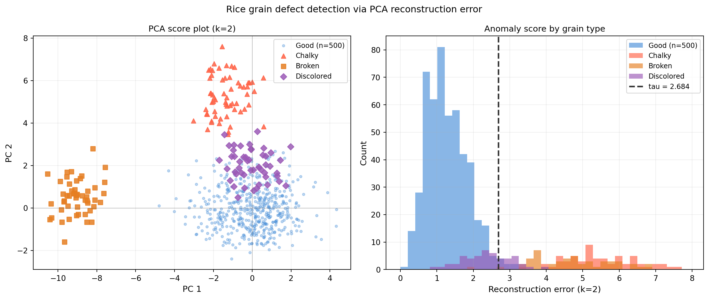
fig, axes = plt.subplots(1, 2, figsize=(13, 5.5))

# Left: PCA score plot (PC1 vs PC2)
ax = axes[0]
ax.scatter(Z_good[:, 0], Z_good[:, 1], s=10, color='#4a90d9', alpha=0.35,
           label=f'Good (n={n_good})')
for name, Xd in X_def.items():
    Zd = project(Xd, mu_hat, std_hat, V)
    ax.scatter(Zd[:, 0], Zd[:, 1], s=35, color=def_colors[name],
               alpha=0.85, marker=def_markers[name], label=name)
ax.axhline(0, color='#333333', lw=0.4, alpha=0.5)
ax.axvline(0, color='#333333', lw=0.4, alpha=0.5)
ax.set_xlabel('PC 1', fontsize=11)
ax.set_ylabel('PC 2', fontsize=11)
ax.set_title('PCA score plot (k=2)', fontsize=11)
ax.legend(fontsize=9)
ax.grid(alpha=0.2)

# Right: reconstruction error histogram
ax2 = axes[1]
all_err = np.concatenate([err_good]
    + [recon_error(X_def[n], mu_hat, std_hat, V) for n in def_colors])
bins = np.linspace(0, max(all_err) * 1.05, 40)
ax2.hist(err_good, bins=bins, color='#4a90d9', alpha=0.65, label=f'Good (n={n_good})')
for name, Xd in X_def.items():
    ax2.hist(recon_error(Xd, mu_hat, std_hat, V),
             bins=bins, color=def_colors[name], alpha=0.65, label=name)
ax2.axvline(tau, color='#333333', lw=2, linestyle='--',
            label=f'tau = {tau:.3f}')
ax2.set_xlabel('Reconstruction error (k=2)', fontsize=11)
ax2.set_ylabel('Count', fontsize=11)
ax2.set_title('Anomaly score by grain type', fontsize=11)
ax2.legend(fontsize=9)
ax2.grid(alpha=0.2)

fig.suptitle('Rice grain defect detection via PCA reconstruction error', fontsize=12)
fig.tight_layout()
plt.savefig('ch20-pca/fig-rice-defects.png', dpi=150, bbox_inches='tight')
plt.show()

20.8.4 Key Takeaways

Standardize before PCA when features have different units. Length (pixels) and chalkiness (fraction) have very different scales; without standardization, length dominates the first PC and chalkiness is invisible.
One-class PCA learns the inlier subspace. We fit PCA only on good grains and use reconstruction error as an anomaly score. Defective grains that do not lie on the good-grain subspace produce large residuals.
Different defects separate differently in PC space. Broken grains (very short) separate cleanly along PC1. Chalky grains separate along the chalkiness-driven PC. Discolored grains are detected via their high reconstruction error even when their PC1-PC2 projection overlaps with good grains.
Choosing \(k\) is a design decision. A smaller \(k\) (fewer components retained) flags more anomalies – including grains that differ only in the discarded dimensions. A larger \(k\) is more permissive. Set \(k\) by the false-positive budget, not by the 90% EVR rule alone.

20.9 Solutions

20.9.1 PCA as Maximum Variance Projection

20.1.1 Let \(z_i = \mathbf{u}^T\tilde{\mathbf{x}}_i\). Because \(\tilde{X}\) is mean-centered, \(\sum_i z_i = \mathbf{u}^T \sum_i \tilde{\mathbf{x}}_i = 0\). Then

\[\text{Var}(\mathbf{u}) = \frac{1}{n-1}\sum_{i=1}^n z_i^2 = \frac{1}{n-1}\sum_i (\mathbf{u}^T\tilde{\mathbf{x}}_i)^2.\]

Write \((\mathbf{u}^T\tilde{\mathbf{x}}_i)^2 = \mathbf{u}^T(\tilde{\mathbf{x}}_i\tilde{\mathbf{x}}_i^T)\mathbf{u}\) (outer product) and sum:

\[\text{Var}(\mathbf{u}) = \mathbf{u}^T \!\left(\frac{1}{n-1}\sum_i \tilde{\mathbf{x}}_i\tilde{\mathbf{x}}_i^T\right)\!\mathbf{u} = \mathbf{u}^T\!\left(\frac{1}{n-1}\tilde{X}^T\tilde{X}\right)\!\mathbf{u} = \mathbf{u}^T\Sigma\mathbf{u}.\]

Note the matrix identity \(\sum_i \tilde{\mathbf{x}}_i\tilde{\mathbf{x}}_i^T = \tilde{X}^T\tilde{X}\) because row \(i\) of \(\tilde{X}\) is \(\tilde{\mathbf{x}}_i^T\).

20.1.2 Without the constraint \(\|\mathbf{u}\|=1\), the objective \(\mathbf{u}^T\Sigma\mathbf{u}\) is unbounded above: replacing \(\mathbf{u}\) by \(c\mathbf{u}\) scales the objective by \(c^2\), which grows without bound as \(c \to \infty\). The unit-norm constraint confines the search to directions (unit vectors) rather than vectors of arbitrary length, making the maximum finite and the solution unique up to sign.

20.1.3 The Lagrangian is \(\mathcal{L} = \mathbf{u}^T\Sigma\mathbf{u} - \lambda(\mathbf{u}^T\mathbf{u}-1)\). Differentiating with respect to \(\mathbf{u}\):

\[\frac{\partial \mathcal{L}}{\partial \mathbf{u}} = 2\Sigma\mathbf{u} - 2\lambda\mathbf{u} = \mathbf{0} \implies \Sigma\mathbf{u} = \lambda\mathbf{u}.\]

At the critical point, the variance achieved is

\[\mathbf{u}^T\Sigma\mathbf{u} = \mathbf{u}^T(\lambda\mathbf{u}) = \lambda\,\mathbf{u}^T\mathbf{u} = \lambda.\]

Therefore, to maximize variance we choose the eigenvector corresponding to the largest eigenvalue \(\lambda_1\).

20.1.4 If \(\lambda_1 = \lambda_2 > \lambda_3\), then every unit vector in the 2D eigenspace \(\text{span}\{\mathbf{q}_1, \mathbf{q}_2\}\) achieves the same variance \(\lambda_1\). The first principal component is not unique; any unit vector in that plane is equally valid. In practice, numerical algorithms return an arbitrary orthonormal basis for the degenerate eigenspace.

20.9.2 PCA via SVD

20.2.1 From \(\tilde{X} = USV^T\):

\[\tilde{X}^T\tilde{X} = (USV^T)^T(USV^T) = VS\underbrace{U^TU}_{=I}SV^T = VS^2V^T.\]

Dividing by \(n-1\): \(\Sigma = V\frac{S^2}{n-1}V^T\). The columns of \(V\) play the role of \(Q\) (eigenvectors), and \(\frac{S^2}{n-1} = \Lambda\) (eigenvalue diagonal).

20.2.2 Direct check: \(\tilde{X}V = (USV^T)V = US\underbrace{V^TV}_{=I} = US\). So \(Z = \tilde{X}V = US\). Both expressions compute identical matrices.

20.2.3 Scaling column \(j\) of \(\tilde{X}\) by 10 multiplies the \(j\)-th component of each row by 10. (a) Singular values change: at minimum, \(\sigma_1\) increases (the scaled column has larger variance). The exact change depends on the eigenvector structure. (b) The first principal direction \(\mathbf{v}_1\) rotates toward the \(\mathbf{e}_j\) direction (feature \(j\) now dominates), especially if the scaled feature was already influential.

20.2.4 With full_matrices=False, the shapes are \(U \in \mathbb{R}^{n \times p}\), \(s \in \mathbb{R}^p\), \(V^T \in \mathbb{R}^{p \times p}\) – the thin SVD. With full_matrices=True, \(U \in \mathbb{R}^{n \times n}\), which for \(n \gg p\) is an enormous matrix we never need. The extra \(n-p\) columns of \(U\) span the left null space of \(\tilde{X}\) and are irrelevant for PCA. The thin SVD saves \(O(n^2 p)\) memory.

20.9.3 Explained Variance and Choosing \(k\)

20.3.1 For \(\Sigma = I_p\), all eigenvalues equal 1. Explained variance ratio: \(r_j = 1/p\) for all \(j\). The scree plot is a flat horizontal line. Cumulative EVR reaches 90% only when \(k \ge 0.9p\) components are retained. White-noise data has no low-dimensional structure; PCA offers no compression.

20.3.2 Using the spectral decomposition \(\Sigma = Q\Lambda Q^T\):

\[\text{tr}(\Sigma) = \text{tr}(Q\Lambda Q^T) = \text{tr}(Q^T Q \Lambda) = \text{tr}(\Lambda) = \sum_j \lambda_j.\]

The second equality uses the cyclic property \(\text{tr}(ABC) = \text{tr}(CAB)\). The third uses \(Q^T Q = I\) (orthogonality).

20.3.3 Squared singular values: \(\sigma_1^2 = 10000\), \(\sigma_2^2 = 400\), \(\sigma_3^2 = \cdots = \sigma_{10}^2 = 25\). Total: \(10000 + 400 + 8 \times 25 = 10600\). EVR: \(r_1 = 10000/10600 \approx 0.943\), \(r_2 = 400/10600 \approx 0.038\), each of \(r_3, \ldots, r_{10} = 25/10600 \approx 0.0024\). Cumulative: \(R_1 \approx 0.943\), \(R_2 \approx 0.981\). So \(k = 1\) already exceeds 94%, and \(k = 2\) exceeds 95%.

20.3.4 Standardization before PCA is equivalent to running PCA on the correlation matrix \(R\) instead of \(\Sigma\). Example: if feature 1 has variance 1000 (large in raw units) and feature 2 has variance 1 (small), raw PCA treats feature 1 as ten times more important regardless of its actual information content. After standardization both features get variance 1 and contribute equally. Result: the two scree plots can point in qualitatively different directions, and the first PC can flip from “mostly feature 1” to “mix of feature 1 and 2.”

20.9.4 Reconstruction and Residuals

20.4.1 \(P_k = V_k V_k^T\). Then \(P_k^2 = V_k V_k^T V_k V_k^T = V_k (V_k^T V_k) V_k^T = V_k I_k V_k^T = P_k\) (since \(V_k^T V_k = I_k\) – columns of \(V_k\) are orthonormal). The complement \(Q_k = I - P_k\) satisfies \(Q_k^2 = I - 2P_k + P_k^2 = I - P_k = Q_k\), so it is also a projection. \(Q_k\) projects onto the orthogonal complement \(\text{span}\{\mathbf{v}_1, \ldots, \mathbf{v}_k\}^\perp = \text{span}\{\mathbf{v}_{k+1}, \ldots, \mathbf{v}_p\}\).

20.4.2 The rank-\(k\) truncated SVD of \(\tilde{X}\) is \(\hat{X}_k = U_k S_k V_k^T\). The residual is \(\tilde{X} - \hat{X}_k = U_{k+:}S_{k+:}V_{k+:}^T\) (tail singular components). Since columns of \([U_k, U_{k+:}]\) and \([V_k, V_{k+:}]\) are each orthonormal, Frobenius squared norm equals the sum of squared singular values: \(\|\tilde{X} - \hat{X}_k\|_F^2 = \sum_{j=k+1}^p \sigma_j^2\).

20.4.3 \(\|\tilde{X}\|_F^2 = 1200\). Top-3 contribution: \(\sigma_1^2 + \sigma_2^2 + \sigma_3^2 = 625 + 225 + 100 = 950\). Residual fraction: \((1200 - 950)/1200 = 250/1200 \approx 0.208\), so about 20.8% of total variance is discarded by \(k=3\).

20.4.4 A large residual \(\|E_{k,i}\|\) means observation \(i\) has a significant component orthogonal to the top-\(k\) PCA subspace – a direction not represented in the inlier data. In anomaly detection this flags the observation as potentially defective: it deviates from the learned low-dimensional structure, even if its projection onto the \(k\)-dim subspace looks normal. This is the basis of PCA-based anomaly detection used in §20.8.

20.9.5 PCA for 3D Point Clouds

20.5.1 Plane fitting minimizes \(\sum_i (\mathbf{n}^T \tilde{\mathbf{p}}_i)^2 = \mathbf{n}^T\Sigma\mathbf{n}\) subject to \(\|\mathbf{n}\|=1\). The Lagrangian is \(\mathbf{n}^T\Sigma\mathbf{n} - \lambda(\mathbf{n}^T\mathbf{n}-1)\) and the critical point satisfies \(\Sigma\mathbf{n} = \lambda\mathbf{n}\). To minimize variance in the normal direction we pick the eigenvector of the smallest eigenvalue. The maximum-variance problem is identical except we want the largest eigenvalue.

20.5.2 If all \(n\) points lie exactly on a plane through the origin, then no point has a component in the normal direction, so \(\mathbf{n}^T\tilde{\mathbf{p}}_i = 0\) for all \(i\). The smallest eigenvalue is exactly \(\lambda_3 = 0\). The rank of \(\Sigma\) is at most 2 (the covariance matrix has a null space in the normal direction), so \(\text{rank}(\Sigma) \le 2\).

20.5.3 Run PCA on each cloud and align the principal axes: compute rotation \(R = V_A V_B^T\) that maps the PC frame of cloud \(A\) to that of cloud \(B\). The remaining ambiguity is sign: each principal axis is defined up to \(\pm\), giving \(2^3 = 8\) possible sign flips. Resolve sign by requiring the rotation matrix to have \(\det(R) = +1\) (proper rotation) and by choosing sign combinations that minimize the residual point-to-point distance after alignment.

20.5.4 Very small \(k\) (e.g., 5 neighbors): the local neighborhood is small and noisy, so the estimated normal has high variance (sensitive to random outliers and quantization noise). Very large \(k\) (e.g., \(n/2\)): the neighborhood spans a large region of the surface, and if the surface curves significantly the patch is not well approximated by a plane, introducing bias (the estimated normal deviates systematically from the true local normal). Optimal \(k\) balances bias and variance, typically chosen via cross-validation or by matching the expected surface curvature to the point cloud density.

20.9.6 Sim-to-Real Domain Adaptation

20.6.1 Let \(\mathbf{f}_s\) be a centered source feature with covariance \(\Sigma_S\). The adapted feature is \(\mathbf{f}_a = M \mathbf{f}_s\) with \(M = \Sigma_T^{1/2}\Sigma_S^{-1/2}\). Its covariance is

\[\text{Cov}(\mathbf{f}_a) = M \Sigma_S M^T = \Sigma_T^{1/2}\Sigma_S^{-1/2}\Sigma_S(\Sigma_S^{-1/2})^T(\Sigma_T^{1/2})^T = \Sigma_T^{1/2} I \Sigma_T^{1/2} = \Sigma_T.\]

(Using symmetry: \(\Sigma_S^{-1/2} = (\Sigma_S^{1/2})^{-1}\) and \((\Sigma_T^{1/2})^T = \Sigma_T^{1/2}\) for symmetric PSD matrices.)

20.6.2 Covariance (second moment) does not capture higher-order statistics: skewness, kurtosis, multimodality, and complex correlations among many features. Two distributions can have identical means and covariances but differ dramatically in their densities. For neural networks, the gap in higher-order statistics, in the frequency content of images, or in the distribution of fine-grained textures may persist even after covariance alignment.

20.6.3 If \(V_S = V_T\), then \(V_S^T V_T = V_S^T V_S = I_k\) (since columns are orthonormal). The SVD of \(I_k\) is \(I = I \cdot I \cdot I\), so all singular values are 1, and \(\theta_j = \arccos(1) = 0\) for all \(j\).

20.6.4 With \(n = 50\) observations and \(p = 20\) features, the sample covariance \(\hat{\Sigma}_T \in \mathbb{R}^{20 \times 20}\) is estimated from \(50 \times 20\) data. Since \(n < 2p\) the sample covariance may be singular or near-singular (rank at most \(n-1 = 49 < p\)), so \(\hat{\Sigma}_T^{-1/2}\) does not exist. Regularize with a ridge term: \(\hat{\Sigma}_T \leftarrow \hat{\Sigma}_T + \epsilon I\) (Ledoit-Wolf shrinkage provides an optimal \(\epsilon\)), or use only the top-\(k\) principal directions of \(\hat{\Sigma}_T\) where \(k \ll n\).

20.9.7 Limitations

20.7.1 Example: two-class data forming concentric rings. The first PC points along the direction of maximum spread of the combined cloud, which is a diameter of the outer ring – irrelevant for classifying inner vs outer. The second PC is orthogonal and similarly useless. No linear PCA direction separates the classes because the class boundary is radial (nonlinear). A kernel PCA with RBF kernel resolves this by mapping to a feature space where the classes are linearly separable.

20.7.2 The corrupted observation contributes \(\mathbf{x}_{\text{corrupt}}\mathbf{x}_{\text{corrupt}}^T = 10000\,\mathbf{e}_1\mathbf{e}_1^T\) to the unnormalized covariance (shift of \(10000/n \approx 10\) in the \((1,1)\) entry of \(\Sigma\)). This inflates \(\lambda_1\) by approximately 10 and rotates \(\mathbf{q}_1\) toward \(\mathbf{e}_1\), regardless of the true data structure. For robust estimation, one would use median-based centering or trim the extreme observations before running PCA.

20.7.3 Height in meters has range 0.5, so variance \(\approx 0.02\). Shoe size has range 12, so variance \(\approx 12\). Unscaled PCA: first PC points almost entirely in the shoe-size direction. After standardization, both features have variance 1 and the first PC captures the genuine correlation between height and shoe size. Numerically, the dot product of the first PC with \(\mathbf{e}_{\text{shoe}}\) drops from near 1 to roughly 0.7 after standardization.

20.7.4 The nuclear norm \(\|L\|_* = \sum_j \sigma_j(L)\) is the convex hull of the rank function on the spectral ball: just as \(\ell_1\) is the convex hull of the cardinality (number of nonzeros) function on the unit \(\ell_\infty\) ball, the nuclear norm is the convex hull of rank on the unit spectral-norm ball. Minimizing \(\|L\|_*\) encourages small singular values – effectively pushing \(L\) toward low rank. Similarly, \(\ell_1\) penalizes the sum of absolute values of entries of \(S\), promoting entries being exactly zero (sparsity) for the same reason that \(\ell_1\) promotes sparsity in LASSO.