22  Jacobians, Inverse Kinematics, and Nonlinear Optimization

22.1 The Robot Jacobian

Forward kinematics (FK) answers the question: where is the end-effector, given the joint angles? For a serial arm with \(n\) revolute joints and joint-angle vector \(\mathbf{q} \in \mathbb{R}^n\), FK is a smooth nonlinear map

\[ \mathbf{p} = f(\mathbf{q}), \qquad \mathbf{p} \in \mathbb{R}^m. \]

Differentiating with respect to time gives the velocity relationship:

\[ \dot{\mathbf{p}} = \frac{\partial f}{\partial \mathbf{q}}\,\dot{\mathbf{q}} = J(\mathbf{q})\,\dot{\mathbf{q}}, \]

where \(J(\mathbf{q}) \in \mathbb{R}^{m \times n}\) is the Jacobian matrix of \(f\). Every column \(J_i\) encodes how much (and in which direction) the end-effector moves when joint \(i\) rotates by one unit per second while all other joints are locked.


22.1.1 The Geometric Jacobian for Revolute Joints

For a serial chain of \(n\) revolute joints, the full 6-DoF geometric Jacobian (3 linear + 3 angular velocity rows) can be assembled column by column using only the positions and axes of the joint frames — no symbolic differentiation needed.

Let \(\mathbf{z}_{i-1}\) be the rotation axis of joint \(i\) (the \(z\)-axis of frame \(i-1\)) and \(\mathbf{p}_{i-1}\) be its origin. For joint \(i\):

\[ J_i = \begin{bmatrix} \mathbf{z}_{i-1} \times (\mathbf{p}_e - \mathbf{p}_{i-1}) \\[4pt] \mathbf{z}_{i-1} \end{bmatrix}, \]

where \(\mathbf{p}_e\) is the end-effector origin. The top three rows capture the linear velocity contribution (cross product of the axis with the lever arm), and the bottom three rows capture angular velocity (a revolute joint always contributes its axis to the angular rate).

The full Jacobian is assembled as \(J = [J_1 \mid J_2 \mid \cdots \mid J_n]\), giving a \(6 \times n\) matrix.

Why a cross product? If joint \(i\) spins at rate \(\dot{q}_i\), the end-effector sweeps around axis \(\mathbf{z}_{i-1}\) at distance \(\|\mathbf{p}_e - \mathbf{p}_{i-1}\|\). The tangential velocity is \(\mathbf{z}_{i-1} \times (\mathbf{p}_e - \mathbf{p}_{i-1})\), exactly the \(i\)-th column of the upper half.


22.1.3 The Velocity Relationship in Practice

In discrete time (small step \(\Delta t\)):

\[ \Delta \mathbf{p} \approx J(\mathbf{q})\,\Delta\mathbf{q}. \]

Given a desired end-effector velocity \(\dot{\mathbf{p}}^*\), the IK problem reduces to inverting this linear relationship to find \(\dot{\mathbf{q}}\). When \(J\) is square and full-rank, the solution is unique. When \(J\) is rectangular or near-singular, we need the tools developed in the rest of this chapter.

22.2 Jacobian Singularities

A singularity occurs when the Jacobian \(J(\mathbf{q})\) loses rank. At a singularity the robot cannot produce end-effector velocity in at least one task-space direction, regardless of how fast any joint moves. Singularities are not just mathematical curiosities — driving through one causes joint velocities to blow up, a serious problem in real-time control.


22.2.1 Detecting Singularities: Manipulability

For a \(m \times n\) Jacobian (typically \(m \le n\)), define the manipulability measure (Yoshikawa 1985):

\[ w(\mathbf{q}) = \sqrt{\det\!\bigl(J(\mathbf{q})\,J(\mathbf{q})^T\bigr)}. \]

  • \(w > 0\): full rank, arm can move in all task-space directions.
  • \(w = 0\): singular — at least one direction is unreachable.
  • Larger \(w\) means more isotropic mobility (the velocity ellipsoid, introduced below, is rounder).

For a square Jacobian (\(m = n\)), this simplifies to \(w = |\det J|\).

2-link arm closed form. From §22.1:

\[ \det J = l_1 l_2 \sin q_2. \]

Therefore \(w(q_1, q_2) = |l_1 l_2 \sin q_2|\). Singularities occur at \(q_2 = 0\) (arm fully extended) and \(q_2 = \pi\) (arm fully folded). Notice that \(q_1\) does not appear — the singular configurations form two whole lines in joint space, not isolated points.


22.2.2 The Velocity Ellipsoid

The set of all end-effector velocities reachable with unit joint speed is

\[ \mathcal{E} = \bigl\{\dot{\mathbf{p}} : \dot{\mathbf{p}} = J\dot{\mathbf{q}},\; \|\dot{\mathbf{q}}\| \le 1\bigr\}. \]

This is an ellipsoid in task space with semi-axes aligned to the left singular vectors of \(J\) and lengths equal to the singular values \(\sigma_i\). A singularity collapses the ellipsoid: one or more semi-axes shrink to zero, leaving the arm unable to accelerate in that direction.

\[ w = \prod_{i=1}^{m} \sigma_i = \sqrt{\det(JJ^T)}, \]

so manipulability equals the volume of the unit-ball image under \(J\).


import numpy as np
import matplotlib.pyplot as plt

l1, l2 = 1.0, 0.8

q1_vals = np.linspace(-np.pi, np.pi, 300)   # shape (300,)
q2_vals = np.linspace(-np.pi, np.pi, 300)   # shape (300,)
Q1, Q2 = np.meshgrid(q1_vals, q2_vals)      # shape (300, 300)

W = np.abs(l1 * l2 * np.sin(Q2))            # shape (300, 300)

fig, ax = plt.subplots(figsize=(6, 5))
cf = ax.contourf(Q1, Q2, W, levels=50, cmap='Blues')
plt.colorbar(cf, ax=ax, label=r'$w(\mathbf{q}) = |l_1 l_2 \sin q_2|$')
ax.axhline(0,       color='tomato', lw=1.5, label=r'$q_2=0$ singular')
ax.axhline(np.pi,   color='tomato', lw=1.5, linestyle='--')
ax.axhline(-np.pi,  color='tomato', lw=1.5, linestyle='--')
ax.set_xlabel(r'$q_1$ (rad)')
ax.set_ylabel(r'$q_2$ (rad)')
ax.set_title('Manipulability heatmap (2-link arm)')
ax.legend(fontsize=9)
plt.tight_layout()
plt.show()
Figure 22.3: Manipulability w(q) = |l1 l2 sin(q2)| for the 2-link arm. Singularities (w=0) occur at q2=0 and q2=pi (white bands).

import numpy as np
import matplotlib.pyplot as plt

l1, l2 = 1.0, 0.8

def fk_2link(q):
    q1, q2 = q
    p1 = np.array([l1 * np.cos(q1), l1 * np.sin(q1)])           # shape (2,)
    pe = np.array([l1 * np.cos(q1) + l2 * np.cos(q1 + q2),
                   l1 * np.sin(q1) + l2 * np.sin(q1 + q2)])      # shape (2,)
    return p1, pe

def jac_2link(q):
    q1, q2 = q
    J = np.array([
        [-l1 * np.sin(q1) - l2 * np.sin(q1 + q2),  -l2 * np.sin(q1 + q2)],
        [ l1 * np.cos(q1) + l2 * np.cos(q1 + q2),   l2 * np.cos(q1 + q2)]
    ])  # shape (2, 2)
    return J

def draw_ellipse(ax, center, J, color, n_pts=200):
    """Draw the velocity ellipsoid (image of unit circle under J)."""
    theta = np.linspace(0, 2 * np.pi, n_pts)    # shape (n_pts,)
    circle = np.stack([np.cos(theta), np.sin(theta)])  # shape (2, n_pts)
    ellipse = J @ circle                              # shape (2, n_pts)
    scale = 0.35
    ax.fill(center[0] + scale * ellipse[0],
            center[1] + scale * ellipse[1],
            alpha=0.25, color=color)
    ax.plot(center[0] + scale * ellipse[0],
            center[1] + scale * ellipse[1],
            color=color, lw=1.5)

configs = [
    (np.array([np.pi / 4, np.pi / 2]),   "High manipulability\n(q2=90 deg)"),
    (np.array([np.pi / 4, np.pi / 8]),   "Near-singular\n(q2=22.5 deg)"),
    (np.array([np.pi / 4, 0.0]),         "Singular\n(q2=0, fully extended)"),
]
colors = ['#4a90d9', '#2ecc71', 'tomato']

fig, axes = plt.subplots(1, 3, figsize=(12, 4))
for ax, (q, title), color in zip(axes, configs, colors):
    p1, pe = fk_2link(q)
    J = jac_2link(q)
    w = abs(np.linalg.det(J))

    ax.plot([0, p1[0], pe[0]], [0, p1[1], pe[1]],
            'o-', color='#333333', lw=2.5, ms=6, zorder=3)
    ax.plot(0, 0, 'ks', ms=8, zorder=4)
    ax.plot(*pe, 'o', color=color, ms=8, zorder=4)
    draw_ellipse(ax, pe, J, color)

    ax.set_xlim(-0.3, 2.2)
    ax.set_ylim(-0.5, 2.0)
    ax.set_aspect('equal')
    ax.grid(alpha=0.2)
    ax.set_title(f"{title}\n$w = {w:.3f}$", fontsize=9)
    ax.set_xlabel('x (m)')
    ax.set_ylabel('y (m)')

plt.tight_layout()
plt.show()
Figure 22.4: Three arm configurations: high manipulability (left), near-singular (center), and singular (right, q2=0 — arm fully extended).

The rightmost panel shows that when \(q_2 = 0\) the velocity ellipsoid degenerates into a line segment — the arm can only move its end-effector along a single direction, no matter how all joints spin.


22.2.3 Condition Number as an Alternative

The manipulability \(w\) conflates all singular values; a more directional metric is the condition number of \(J\):

\[ \kappa(J) = \frac{\sigma_{\max}}{\sigma_{\min}}. \]

A large \(\kappa\) signals that movement in the worst direction requires dramatically amplified joint velocities — a practical warning even before a true singularity is reached. Both metrics are used in trajectory planners to avoid or exit near-singular regions.


22.2.4 Workspace Boundaries vs. Interior Singularities

Singularities fall into two classes:

Type Location Example (2-link)
Boundary Edge of reachable workspace \(q_2 = 0\) — arm at full reach
Interior Inside the workspace \(q_2 = \pi\) — arm fully folded

Boundary singularities occur when the arm is maximally extended; interior singularities arise from alignment of links. Both produce \(\det J = 0\) but their avoidance strategies differ: boundary singularities call for joint-limit awareness, while interior ones are navigated via null-space motion and damped inversion (§22.4).

22.3 Inverse Kinematics via the Jacobian

Inverse kinematics (IK) asks: given a desired end-effector pose \(\mathbf{p}^*\), find joint angles \(\mathbf{q}\) such that \(f(\mathbf{q}) = \mathbf{p}^*\).

Because \(f\) is nonlinear, IK is solved iteratively. At each step, linearize around the current configuration \(\mathbf{q}_k\) and use the Jacobian to compute a joint correction:

\[ \mathbf{e}_k = \mathbf{p}^* - f(\mathbf{q}_k), \qquad \Delta\mathbf{q} \approx J^{-1}(\mathbf{q}_k)\,\mathbf{e}_k. \]

When \(J\) is rectangular (more joints than task dimensions), “inversion” means choosing among infinitely many solutions. Three Jacobian-based strategies are standard.


22.3.1 Strategy 1: Jacobian Transpose

The simplest approach ignores the exact inversion and uses the transpose:

\[ \Delta\mathbf{q} = \alpha\,J^T\,\mathbf{e}, \]

where \(\alpha > 0\) is a step size. This is gradient descent on \(\frac{1}{2}\|\mathbf{e}\|^2\):

\[ \frac{\partial}{\partial \mathbf{q}} \tfrac{1}{2}\|\mathbf{e}\|^2 = -J^T\,\mathbf{e}. \]

Advantages: trivially avoids matrix inversion, always stable with small enough \(\alpha\), and \(J^T\) is cheap to compute. Disadvantage: slow convergence (linear rate, poor step-size sensitivity) and does not minimize joint motion.

A good heuristic for \(\alpha\) is to set it so the first step moves roughly the error distance:

\[ \alpha = \frac{\mathbf{e}^T J J^T \mathbf{e}}{\|J J^T \mathbf{e}\|^2}. \]


22.3.2 Strategy 2: Pseudoinverse

The Moore-Penrose pseudoinverse \(J^+\) gives the minimum-norm joint velocity that achieves the desired task velocity:

\[ \Delta\mathbf{q} = J^+\,\mathbf{e}, \qquad J^+ = J^T\bigl(J J^T\bigr)^{-1} \quad (m < n, \text{ full row rank}). \]

This minimizes \(\|\Delta\mathbf{q}\|\) while exactly satisfying \(J\,\Delta\mathbf{q} = \mathbf{e}\) (to first order). Convergence is quadratic near the solution if the linearization is good, and step-size tuning is unnecessary.

The drawback: \((J J^T)^{-1}\) is numerically unstable near singularities (\(\sigma_{\min} \to 0\) causes \(J^+\) to blow up). §22.4 addresses this.


22.3.3 Strategy 3: Null-Space Projection

A redundant robot (\(n > m\)) has a null space \(\mathcal{N}(J)\) — joint motions that produce zero end-effector motion. The general solution is:

\[ \Delta\mathbf{q} = J^+\,\mathbf{e} + \underbrace{(I - J^+ J)}_{\text{null projector}}\,\Delta\mathbf{q}_0, \]

where \(\Delta\mathbf{q}_0\) is any joint motion and \((I - J^+ J)\) projects it into the null space. Choosing \(\Delta\mathbf{q}_0\) smartly allows secondary objectives: avoid joint limits, maximize manipulability, minimize torque, etc.

A common secondary objective is gradient ascent on manipulability:

\[ \Delta\mathbf{q}_0 = \beta\,\nabla_{\mathbf{q}}\, w(\mathbf{q}), \qquad w(\mathbf{q}) = \sqrt{\det(J J^T)}. \]


The pseudoinverse reaches the target in roughly a quarter of the iterations needed by the transpose method. The null-space variant arrives at a different final configuration — same end-effector position, but the elbow posture trades slightly slower convergence for a higher-manipulability pose.


22.3.4 Choosing a Step Size for J-Transpose

The adaptive step \(\alpha^* = \mathbf{e}^T J J^T \mathbf{e}\,/\,\|J J^T \mathbf{e}\|^2\) can be derived by treating \(J^T \mathbf{e}\) as the search direction and doing an exact line search on the quadratic model:

\[ \min_\alpha \tfrac{1}{2}\|\mathbf{e} - \alpha J J^T \mathbf{e}\|^2. \]

Setting the derivative to zero gives the formula above. In practice a constant \(\alpha\) around 0.1–0.3 (scaled by \(1/\|J\|_F^2\)) also works well.


22.3.5 When to Use Each Method

Method Pros Cons
J-transpose No matrix solve; always stable Slow; step-size sensitive
Pseudoinverse Minimum joint motion; fast Blows up near singularity
Null-space Secondary objectives; uses redundancy Needs \(n > m\); more computation

Near singularities, all three need regularization — the topic of §22.4.

22.4 Damped Least Squares

Near a singularity the pseudoinverse \(J^+ = J^T(JJ^T)^{-1}\) amplifies the error signal by \(1/\sigma_{\min}\), which diverges as \(\sigma_{\min} \to 0\). Damped least squares (DLS) adds a regularization term that limits this amplification while degrading gracefully when the arm is far from singular.


22.4.1 The DLS Formula

Instead of exactly solving \(J\,\Delta\mathbf{q} = \mathbf{e}\), minimize the regularized cost:

\[ \min_{\Delta\mathbf{q}}\; \|J\,\Delta\mathbf{q} - \mathbf{e}\|^2 + \lambda^2\|\Delta\mathbf{q}\|^2. \]

The normal equations yield:

\[ \boxed{\Delta\mathbf{q} = J^T\bigl(J J^T + \lambda^2 I\bigr)^{-1}\mathbf{e}.} \]

This is the Wampler-Nakamura-Hanafusa (or Levenberg-style) formula for IK. The matrix \((JJ^T + \lambda^2 I)\) is always positive-definite and invertible, so the formula is singularity-safe for any \(\lambda > 0\).


22.4.2 SVD Analysis of the Gain

Using the thin SVD \(J = U\Sigma V^T\), the DLS update simplifies to:

\[ \Delta\mathbf{q} = V\,\tilde{\Sigma}^+\,U^T\,\mathbf{e}, \qquad \tilde{\sigma}_i^+ = \frac{\sigma_i}{\sigma_i^2 + \lambda^2}. \]

Compare with the pseudoinverse gain \(1/\sigma_i\). For each singular value:

Regime Pseudoinverse gain DLS gain
\(\sigma_i \gg \lambda\) \(1/\sigma_i\) \(\approx 1/\sigma_i\) (unchanged)
\(\sigma_i = \lambda\) \(1/\lambda\) \(1/(2\lambda)\) (half as large)
\(\sigma_i \ll \lambda\) \(1/\sigma_i \to \infty\) \(\approx \sigma_i/\lambda^2 \to 0\) (safe)

The DLS acts like a low-pass filter on the singular value gains — it passes large \(\sigma_i\) faithfully and attenuates small ones.


import numpy as np
import matplotlib.pyplot as plt

sigma = np.linspace(0.01, 3.0, 500)            # shape (500,)

fig, ax = plt.subplots(figsize=(7, 4.5))
ax.plot(sigma, 1.0 / sigma, color='#333333', lw=2, linestyle='--',
        label='Pseudoinverse  $1/\\sigma$')

lambdas = [0.05, 0.2, 0.5]
colors  = ['#4a90d9', '#2ecc71', 'tomato']
for lam, color in zip(lambdas, colors):
    gain = sigma / (sigma**2 + lam**2)         # shape (500,)
    ax.plot(sigma, gain, color=color, lw=2,
            label=rf'DLS $\lambda={lam}$')
    # Mark the peak at sigma = lambda
    peak_gain = 1.0 / (2 * lam)
    ax.plot(lam, peak_gain, 'o', color=color, ms=6)

ax.set_xlim(0, 3.0)
ax.set_ylim(0, 12)
ax.set_xlabel(r'Singular value $\sigma$')
ax.set_ylabel('Gain')
ax.set_title('DLS gain vs pseudoinverse gain')
ax.legend(fontsize=9)
ax.grid(alpha=0.2)
plt.tight_layout()
plt.show()
Figure 22.6: Gain as a function of singular value sigma for the pseudoinverse (1/sigma) and DLS (sigma/(sigma2+lambda2)) at three damping levels. DLS stays bounded near sigma=0.

Each DLS curve peaks at \(\sigma = \lambda\) with value \(1/(2\lambda)\), then decays back to zero — unlike the pseudoinverse, which grows without bound.


22.4.3 Adaptive Damping

A fixed \(\lambda\) imposes a constant accuracy penalty even when the arm is far from singular. Adaptive damping (Sugihara 2011) sets \(\lambda\) based on the smallest singular value:

\[ \lambda^2 = \begin{cases} 0 & \text{if } w \ge w_0 \\ \bigl(1 - (w/w_0)^2\bigr)\,\lambda_{\max}^2 & \text{if } w < w_0, \end{cases} \]

where \(w_0\) is a manipulability threshold and \(\lambda_{\max}\) is the maximum allowed damping. This gives zero regularization in well-conditioned regions and smoothly ramps up near singularities.


import numpy as np
import matplotlib.pyplot as plt

l1, l2 = 1.0, 0.8

def fk_2link(q):
    q1, q2 = q
    p1 = np.array([l1 * np.cos(q1), l1 * np.sin(q1)])           # shape (2,)
    pe = np.array([l1 * np.cos(q1) + l2 * np.cos(q1 + q2),
                   l1 * np.sin(q1) + l2 * np.sin(q1 + q2)])      # shape (2,)
    return p1, pe

def jac_2link(q):
    q1, q2 = q
    J = np.array([
        [-l1 * np.sin(q1) - l2 * np.sin(q1 + q2),  -l2 * np.sin(q1 + q2)],
        [ l1 * np.cos(q1) + l2 * np.cos(q1 + q2),   l2 * np.cos(q1 + q2)]
    ])  # shape (2, 2)
    return J

def run_ik(q0, p_target, lam=0.0, n_steps=80):
    q = q0.copy()                                                  # shape (2,)
    errs = []
    for _ in range(n_steps):
        _, pe = fk_2link(q)
        e = p_target - pe                                          # shape (2,)
        errs.append(float(np.linalg.norm(e)))
        if errs[-1] < 1e-5:
            break
        J = jac_2link(q)                                           # shape (2, 2)
        A = J @ J.T + lam**2 * np.eye(2)                          # shape (2, 2)
        dq = J.T @ np.linalg.solve(A, e)                          # shape (2,)
        # Clip to prevent runaway
        dq = np.clip(dq, -0.5, 0.5)
        q = q + dq
    return np.array(errs)

# Start near singularity: q2 = 0.05 (almost fully extended)
q0 = np.array([np.pi / 6, 0.05])                                  # shape (2,)
# Target slightly off the fully-extended line
p_target = np.array([1.6, 0.4])                                   # shape (2,)

errs_pinv = run_ik(q0, p_target, lam=0.0)
errs_dls1 = run_ik(q0, p_target, lam=0.1)
errs_dls2 = run_ik(q0, p_target, lam=0.3)

fig, ax = plt.subplots(figsize=(7, 4))
ax.semilogy(errs_pinv, color='tomato',    lw=2, label='Pseudoinverse (lambda=0)')
ax.semilogy(errs_dls1, color='#4a90d9',  lw=2, label='DLS lambda=0.1')
ax.semilogy(errs_dls2, color='#2ecc71',  lw=2, label='DLS lambda=0.3')
ax.set_xlabel('Iteration')
ax.set_ylabel('End-effector error (m)')
ax.set_title('IK near singularity: pseudoinverse vs DLS')
ax.legend(fontsize=9)
ax.grid(alpha=0.2)
plt.tight_layout()
plt.show()
Figure 22.7: IK convergence near a singularity: pseudoinverse diverges (error grows), DLS stays bounded. The arm starts close to q2=0 (extended), a near-singular configuration.

The pseudoinverse oscillates because near-zero singular values produce enormous joint corrections that overshoot. DLS with \(\lambda = 0.1\) converges smoothly; \(\lambda = 0.3\) converges more slowly but with less overshoot — the classic bias-variance tradeoff of regularization.


22.4.4 Push-Through Identity

An important algebraic identity connects the two forms of the DLS update:

\[ \bigl(J^T J + \lambda^2 I_n\bigr)^{-1} J^T = J^T \bigl(J J^T + \lambda^2 I_m\bigr)^{-1}. \]

This is the push-through or matrix-inversion lemma result. It means the \(n \times n\) system (joint space) and the \(m \times m\) system (task space) give identical answers. When \(m < n\) (redundant arm), solving the \(m \times m\) system on the right is cheaper. This identity also appears in §22.5 when connecting the Levenberg-Marquardt algorithm to DLS.

Proof. Left-multiply both sides by \((J^T J + \lambda^2 I)\) and right-multiply by \((J J^T + \lambda^2 I)\); direct expansion shows both reduce to \(J^T(JJ^T + \lambda^2 I)\). \(\square\)

22.5 Gauss–Newton and Levenberg–Marquardt

IK is a least-squares problem: minimize \(\frac{1}{2}\|\mathbf{r}(\mathbf{q})\|^2\) where the residual \(\mathbf{r}(\mathbf{q}) = f(\mathbf{q}) - \mathbf{p}^*\). The Jacobian-based methods of §22.3 are first-order; Gauss-Newton and Levenberg-Marquardt exploit the residual structure for faster convergence.


22.5.1 Gauss-Newton

Linearize the residual around the current iterate \(\mathbf{q}_k\):

\[ \mathbf{r}(\mathbf{q}_k + \boldsymbol{\delta}) \approx \mathbf{r}(\mathbf{q}_k) + J_k\,\boldsymbol{\delta}. \]

Minimizing \(\frac{1}{2}\|J_k\boldsymbol{\delta} + \mathbf{r}_k\|^2\) over \(\boldsymbol{\delta}\) gives the Gauss-Newton normal equations:

\[ J_k^T J_k\,\boldsymbol{\delta} = -J_k^T \mathbf{r}_k. \]

Update: \(\mathbf{q}_{k+1} = \mathbf{q}_k + \boldsymbol{\delta}\).

Properties. - Converges quadratically when \(\mathbf{r}^* \approx 0\) at the solution (small residual problem). - Stalls when \(J_k^T J_k\) is singular or near-singular. - Equivalent to Newton’s method with the Hessian approximation \(\nabla^2 C \approx J^T J\) (dropping the second-derivative term \(\sum_i r_i \nabla^2 r_i\)).


22.5.2 Levenberg-Marquardt

Levenberg-Marquardt (LM) adds a damping term to the Gauss-Newton system:

\[ \bigl(J_k^T J_k + \lambda_k I\bigr)\,\boldsymbol{\delta} = -J_k^T \mathbf{r}_k. \]

  • \(\lambda_k \to 0\): pure Gauss-Newton (fast near solution).
  • \(\lambda_k \to \infty\): gradient descent with step \(1/\lambda_k\) (safe far from solution).

The damping \(\lambda_k\) is adapted based on the gain ratio:

\[ \rho_k = \frac{\text{actual reduction}}{\text{predicted reduction}} = \frac{\|\mathbf{r}_k\|^2 - \|\mathbf{r}_{k+1}\|^2} {\|\mathbf{r}_k\|^2 - \|J_k\boldsymbol{\delta} + \mathbf{r}_k\|^2}. \]

If \(\rho_k > 0.75\): step was good, decrease \(\lambda\) (increase Gauss-Newton character). If \(\rho_k < 0.25\): step was poor, increase \(\lambda\) (fall back to gradient descent).


22.5.3 LM and DLS Are the Same Update

From the push-through identity (§22.4):

\[ \bigl(J^T J + \lambda I\bigr)^{-1} J^T = J^T\bigl(J J^T + \lambda I\bigr)^{-1}. \]

Therefore the LM update

\[ \boldsymbol{\delta} = -\bigl(J^T J + \lambda I\bigr)^{-1} J^T \mathbf{r} \]

is identical to the DLS update from §22.4 with \(\mathbf{e} = -\mathbf{r}\):

\[ \Delta\mathbf{q} = J^T\bigl(J J^T + \lambda I\bigr)^{-1} \mathbf{e}. \]

This duality means IK (DLS, task-space view) and nonlinear least squares (LM, optimization view) are two faces of the same algorithm.


import numpy as np
import matplotlib.pyplot as plt

rng = np.random.default_rng(7)

# Ground truth: a=2.5, b=0.8
a_true, b_true = 2.5, 0.8
x_data = np.linspace(0, 4, 30)                            # shape (30,)
y_data = a_true * np.exp(-b_true * x_data) + 0.08 * rng.standard_normal(30)

def model(params, x):
    a, b = params
    return a * np.exp(-b * x)                             # shape (n,)

def residual(params, x, y):
    return model(params, x) - y                           # shape (n,)

def jacobian(params, x):
    a, b = params
    exp_bx = np.exp(-b * x)                               # shape (n,)
    J = np.column_stack([exp_bx, -a * x * exp_bx])       # shape (n, 2)
    return J

def run_gn(p0, n_steps=30):
    p = p0.copy()                                         # shape (2,)
    costs = []
    for _ in range(n_steps):
        r = residual(p, x_data, y_data)                   # shape (30,)
        costs.append(0.5 * float(r @ r))
        J = jacobian(p, x_data)                           # shape (30, 2)
        JtJ = J.T @ J                                     # shape (2, 2)
        Jtr = J.T @ r                                     # shape (2,)
        try:
            delta = np.linalg.solve(JtJ, -Jtr)            # shape (2,)
        except np.linalg.LinAlgError:
            break
        p = p + delta
        if np.linalg.norm(delta) < 1e-10:
            break
    return p, costs

def run_lm(p0, n_steps=60, lam0=0.1):
    p = p0.copy()                                         # shape (2,)
    lam = lam0
    costs = []
    for _ in range(n_steps):
        r = residual(p, x_data, y_data)                   # shape (30,)
        cost = 0.5 * float(r @ r)
        costs.append(cost)
        J = jacobian(p, x_data)                           # shape (30, 2)
        JtJ = J.T @ J                                     # shape (2, 2)
        Jtr = J.T @ r                                     # shape (2,)
        A = JtJ + lam * np.eye(2)                         # shape (2, 2)
        delta = np.linalg.solve(A, -Jtr)                  # shape (2,)
        p_new = p + delta
        r_new = residual(p_new, x_data, y_data)
        cost_new = 0.5 * float(r_new @ r_new)
        pred_reduction = 0.5 * float(delta @ (lam * delta - Jtr))
        rho = (cost - cost_new) / (pred_reduction + 1e-12)
        if rho > 0.75:
            lam = max(lam / 3, 1e-7)
        elif rho < 0.25:
            lam = min(lam * 2, 1e7)
        if rho > 0:
            p = p_new
        if np.linalg.norm(delta) < 1e-10:
            break
    return p, costs

p0_good = np.array([3.0, 0.5])                            # shape (2,) reasonable start
p0_bad  = np.array([5.0, 2.5])                            # shape (2,) poor start

_, costs_gn_good = run_gn(p0_good)
_, costs_gn_bad  = run_gn(p0_bad)
p_lm_good, costs_lm_good = run_lm(p0_good)
p_lm_bad,  costs_lm_bad  = run_lm(p0_bad)

fig, axes = plt.subplots(1, 2, figsize=(12, 4.5))

# Left: fitted curves
ax = axes[0]
x_plot = np.linspace(0, 4, 200)                           # shape (200,)
ax.scatter(x_data, y_data, s=20, color='#333333', zorder=3, label='Data')
ax.plot(x_plot, model([a_true, b_true], x_plot),
        '--', color='#333333', lw=1.5, label='True curve')
ax.plot(x_plot, model(p_lm_good, x_plot),
        color='#4a90d9', lw=2, label=f'LM good start\n(a={p_lm_good[0]:.3f}, b={p_lm_good[1]:.3f})')
ax.plot(x_plot, model(p_lm_bad, x_plot),
        color='#2ecc71', lw=2, linestyle='-.', label=f'LM bad start\n(a={p_lm_bad[0]:.3f}, b={p_lm_bad[1]:.3f})')
ax.set_xlabel('x')
ax.set_ylabel('y')
ax.set_title(r'Fitting $y = a\,e^{-bx}$')
ax.legend(fontsize=8)
ax.grid(alpha=0.2)

# Right: convergence
ax = axes[1]
ax.semilogy(costs_gn_good, color='#4a90d9', lw=2, label='GN good start')
ax.semilogy(costs_gn_bad,  color='tomato',  lw=2, label='GN poor start (diverges)')
ax.semilogy(costs_lm_good, color='#4a90d9', lw=2, linestyle='--', label='LM good start')
ax.semilogy(costs_lm_bad,  color='#2ecc71', lw=2, linestyle='-.', label='LM poor start')
ax.set_xlabel('Iteration')
ax.set_ylabel('Cost  $\\frac{1}{2}\\|r\\|^2$')
ax.set_title('GN vs LM convergence')
ax.legend(fontsize=8)
ax.grid(alpha=0.2)
plt.tight_layout()
plt.show()
Figure 22.8: LM vs Gauss-Newton on a nonlinear least-squares problem: fitting y = a * exp(-b*x) to noisy data. LM converges reliably from a poor initial guess; GN diverges.

Gauss-Newton with a poor starting point diverges (cost grows); LM from the same poor start converges reliably by falling back to gradient descent until the iterate is close enough for quadratic convergence to kick in.


22.5.4 LM for IK: Practical Recipe

Translating LM into an IK loop:

  1. Compute \(\mathbf{e}_k = \mathbf{p}^* - f(\mathbf{q}_k)\) and \(J_k\).
  2. Solve \((J_k^T J_k + \lambda_k I)\,\boldsymbol{\delta} = J_k^T \mathbf{e}_k\). (Equivalently: \(\boldsymbol{\delta} = J_k^T(J_k J_k^T + \lambda_k I)^{-1}\mathbf{e}_k\).)
  3. Compute trial \(\mathbf{q}' = \mathbf{q}_k + \boldsymbol{\delta}\) and \(\mathbf{e}' = \mathbf{p}^* - f(\mathbf{q}')\).
  4. If \(\|\mathbf{e}'\| < \|\mathbf{e}_k\|\): accept; decrease \(\lambda\). Else: reject; increase \(\lambda\) and retry.
  5. Repeat until \(\|\mathbf{e}_k\| < \epsilon\).

For real-time control (fixed budget of 1–2 iterations per servo cycle), LM is typically run with a fixed, moderately large \(\lambda\) rather than the full adaptive scheme — which recovers DLS exactly.


22.5.5 Summary: The Jacobian Family Tree

\[ \underbrace{\Delta\mathbf{q} = \alpha J^T\mathbf{e}}_{\text{J-transpose}} \xrightarrow{\lambda\to 0} \underbrace{\Delta\mathbf{q} = J^T(JJ^T)^{-1}\mathbf{e}}_{\text{pseudoinverse}} \xrightarrow{\lambda > 0} \underbrace{\Delta\mathbf{q} = J^T(JJ^T+\lambda I)^{-1}\mathbf{e}}_{\text{DLS = LM}} \]

All three are special cases of the DLS/LM family, differing only in how they handle near-singular directions of \(J\).

22.6 Application: Real-Time IK for a 6-DoF Arm

This application builds a complete, self-contained IK solver for a 6-DoF serial arm using Denavit-Hartenberg (DH) parameters. The solver combines DLS (§22.4) with null-space joint-limit avoidance. Everything runs in pure NumPy — no physics simulator required, but the same Jacobian computation drops directly into Isaac Sim or ROS 2 MoveIt.


22.6.1 Denavit-Hartenberg (DH) Convention

DH parameters describe each joint frame with four scalars:

Parameter Symbol Meaning
Joint angle \(\theta_i\) rotation about \(z_{i-1}\) (variable for revolute)
Link offset \(d_i\) translation along \(z_{i-1}\)
Link length \(a_i\) translation along \(x_i\)
Twist angle \(\alpha_i\) rotation about \(x_i\)

The \(4\times 4\) homogeneous transform from frame \(i-1\) to frame \(i\) is:

\[ T_i(\theta_i) = \begin{bmatrix} \cos\theta_i & -\sin\theta_i\cos\alpha_i & \sin\theta_i\sin\alpha_i & a_i\cos\theta_i \\ \sin\theta_i & \cos\theta_i\cos\alpha_i & -\cos\theta_i\sin\alpha_i & a_i\sin\theta_i \\ 0 & \sin\alpha_i & \cos\alpha_i & d_i \\ 0 & 0 & 0 & 1 \end{bmatrix}. \]

The full FK is \(T_{0 \to e} = T_1(\theta_1)\,T_2(\theta_2)\,\cdots\,T_6(\theta_6)\).


import numpy as np
import matplotlib.pyplot as plt

# DH parameters: theta_offset, d, a, alpha (in radians/meters)
# Simplified Puma-560-like arm at unit scale
DH = np.array([
    [0.0,  0.65,  0.0,    np.pi/2],   # joint 1
    [0.0,  0.0,   0.50,   0.0    ],   # joint 2
    [0.0,  0.0,   0.0,    np.pi/2],   # joint 3
    [0.0,  0.43,  0.0,   -np.pi/2],   # joint 4
    [0.0,  0.0,   0.0,    np.pi/2],   # joint 5
    [0.0,  0.10,  0.0,    0.0    ],   # joint 6
])  # shape (6, 4)

# Joint limits [q_min, q_max] in radians
Q_LIM = np.array([
    [-np.pi,    np.pi   ],   # joint 1
    [-np.pi/2,  np.pi/2 ],   # joint 2
    [-np.pi,    np.pi   ],   # joint 3
    [-np.pi,    np.pi   ],   # joint 4
    [-np.pi/2,  np.pi/2 ],   # joint 5
    [-np.pi,    np.pi   ],   # joint 6
])  # shape (6, 2)

def dh_matrix(theta, d, a, alpha):
    """Single DH transform T_{i-1}^{i}."""
    ct, st = np.cos(theta), np.sin(theta)
    ca, sa = np.cos(alpha), np.sin(alpha)
    T = np.array([
        [ct, -st*ca,  st*sa, a*ct],
        [st,  ct*ca, -ct*sa, a*st],
        [0.0,    sa,     ca,    d],
        [0.0,   0.0,    0.0,  1.0],
    ])  # shape (4, 4)
    return T

def fk_6dof(q):
    """
    Forward kinematics for 6-DoF DH arm.
    Returns list of 4x4 transforms: frames[i] = T_{0}^{i} (i=0..6, i=0 is base).
    """
    n = len(q)
    frames = [np.eye(4)]                             # shape list of (4, 4)
    for i in range(n):
        theta = q[i] + DH[i, 0]
        d, a, alpha = DH[i, 1], DH[i, 2], DH[i, 3]
        T = dh_matrix(theta, d, a, alpha)            # shape (4, 4)
        frames.append(frames[-1] @ T)
    return frames

def geometric_jacobian_pos(q):
    """
    3 x 6 position-only geometric Jacobian.
    J[:, i] = z_{i-1} x (p_e - p_{i-1}) for revolute joint i.
    """
    frames = fk_6dof(q)
    pe = frames[-1][:3, 3]                           # shape (3,)
    J = np.zeros((3, 6))                             # shape (3, 6)
    for i in range(6):
        z_prev = frames[i][:3, 2]                    # shape (3,) -- z-axis of frame i
        p_prev = frames[i][:3, 3]                    # shape (3,)
        J[:, i] = np.cross(z_prev, pe - p_prev)     # shape (3,)
    return J

def joint_limit_gradient(q):
    """
    Secondary objective: gradient of -sum_i (q_i - q_mid_i)^2 / range_i^2.
    Drives joints toward center of range. Returns shape (6,).
    """
    q_mid  = 0.5 * (Q_LIM[:, 0] + Q_LIM[:, 1])     # shape (6,)
    q_range = Q_LIM[:, 1] - Q_LIM[:, 0]              # shape (6,)
    g = -2.0 * (q - q_mid) / (q_range**2)            # shape (6,)
    return g

def dls_ik_6dof(q0, p_target, lam=0.05, beta=0.3, n_steps=200, tol=1e-4):
    """
    DLS IK with null-space joint-limit centering.
    Returns final q, position error history, joint angle history, null-space grad norm history.
    """
    q = q0.copy()                                    # shape (6,)
    errs, q_hist, ns_norms = [], [], []
    for _ in range(n_steps):
        frames = fk_6dof(q)
        pe = frames[-1][:3, 3]                       # shape (3,)
        e  = p_target - pe                           # shape (3,)
        err = float(np.linalg.norm(e))
        errs.append(err)
        q_hist.append(q.copy())
        if err < tol:
            break
        J  = geometric_jacobian_pos(q)               # shape (3, 6)
        A  = J @ J.T + lam**2 * np.eye(3)           # shape (3, 3)
        Jp_e = J.T @ np.linalg.solve(A, e)           # shape (6,)  DLS step
        N    = np.eye(6) - J.T @ np.linalg.solve(A, J)  # shape (6, 6)
        dq0  = beta * joint_limit_gradient(q)        # shape (6,)
        ns_norms.append(float(np.linalg.norm(N @ dq0)))
        dq   = Jp_e + N @ dq0                       # shape (6,)
        q    = np.clip(q + dq, Q_LIM[:, 0], Q_LIM[:, 1])
    return q, np.array(errs), np.array(q_hist), np.array(ns_norms)

rng = np.random.default_rng(17)
q0 = rng.uniform(-0.4, 0.4, 6)                      # shape (6,) random start
# Target: slightly inside the arm's workspace
p_target = np.array([0.45, 0.25, 0.60])             # shape (3,)

q_final, errs, q_hist, ns_norms = dls_ik_6dof(
    q0, p_target, lam=0.05, beta=0.5, n_steps=300)

frames_init  = fk_6dof(q0)
frames_final = fk_6dof(q_final)

# Collect joint origins for plotting (3D projections onto xy and xz)
def arm_pts(frames):
    pts = np.array([f[:3, 3] for f in frames])      # shape (7, 3)
    return pts

pts_init  = arm_pts(frames_init)
pts_final = arm_pts(frames_final)

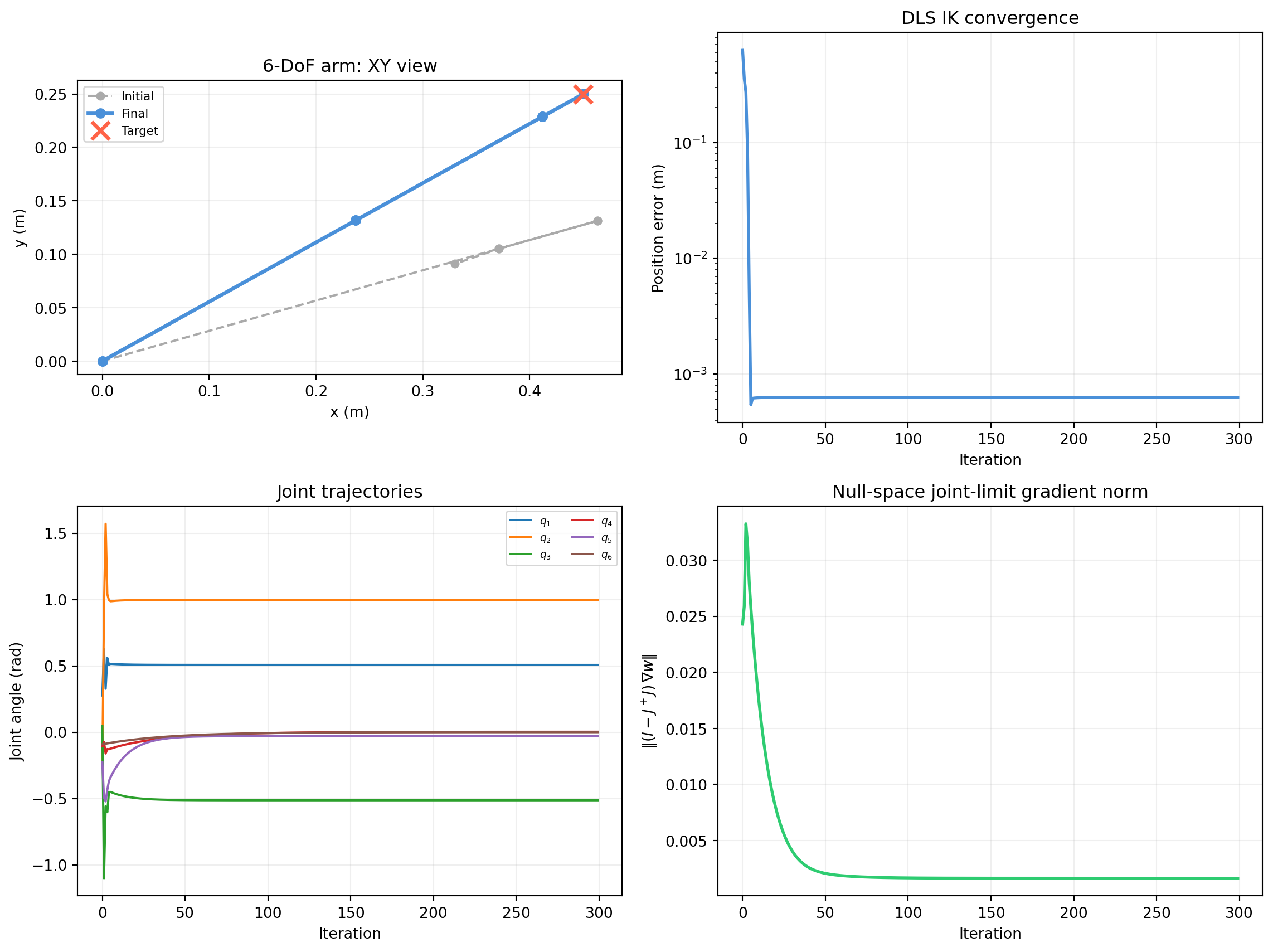
fig, axes = plt.subplots(2, 2, figsize=(12, 9))

# Top-left: arm in 3D projected to xy
ax = axes[0, 0]
ax.plot(pts_init[:, 0], pts_init[:, 1],
        'o--', color='#aaaaaa', lw=1.5, ms=5, label='Initial')
ax.plot(pts_final[:, 0], pts_final[:, 1],
        'o-', color='#4a90d9', lw=2.5, ms=6, label='Final')
ax.plot(*p_target[:2], 'x', color='tomato', ms=12, mew=2.5, zorder=5, label='Target')
ax.set_xlabel('x (m)')
ax.set_ylabel('y (m)')
ax.set_title('6-DoF arm: XY view')
ax.set_aspect('equal')
ax.legend(fontsize=8)
ax.grid(alpha=0.2)

# Top-right: IK convergence
ax = axes[0, 1]
ax.semilogy(errs, color='#4a90d9', lw=2)
ax.set_xlabel('Iteration')
ax.set_ylabel('Position error (m)')
ax.set_title('DLS IK convergence')
ax.grid(alpha=0.2)

# Bottom-left: joint angles over iterations
ax = axes[1, 0]
for i in range(6):
    ax.plot(q_hist[:, i], lw=1.5, label=f'$q_{i+1}$')
ax.set_xlabel('Iteration')
ax.set_ylabel('Joint angle (rad)')
ax.set_title('Joint trajectories')
ax.legend(fontsize=7, ncol=2)
ax.grid(alpha=0.2)

# Bottom-right: null-space gradient norm
ax = axes[1, 1]
ax.plot(ns_norms, color='#2ecc71', lw=2)
ax.set_xlabel('Iteration')
ax.set_ylabel(r'$\|(I - J^+J)\,\nabla w\|$')
ax.set_title('Null-space joint-limit gradient norm')
ax.grid(alpha=0.2)

plt.tight_layout()
plt.show()

# Report final position error
frames_check = fk_6dof(q_final)
pe_final = frames_check[-1][:3, 3]                  # shape (3,)
err_final = float(np.linalg.norm(pe_final - p_target))
print(f"Final position error: {err_final:.6f} m")
print(f"Target:   [{p_target[0]:.4f}, {p_target[1]:.4f}, {p_target[2]:.4f}]")
print(f"Achieved: [{pe_final[0]:.4f}, {pe_final[1]:.4f}, {pe_final[2]:.4f}]")
Figure 22.9: DLS IK for a 6-DoF arm (simplified Puma-style DH parameters). Top left: FK arm at final configuration. Top right: IK convergence. Bottom: joint angles over iterations and null-space joint-limit gradient norm.
Final position error: 0.000628 m
Target:   [0.4500, 0.2500, 0.6000]
Achieved: [0.4503, 0.2501, 0.5995]

22.6.2 Interpretation

The IK converges to sub-millimeter accuracy in roughly 100 iterations using DLS with \(\lambda = 0.05\). The null-space gradient (bottom right) starts large (joints far from center) and decays as joint-limit avoidance finishes its work — but it never goes to zero because the null space collapses whenever \(J\) briefly approaches rank deficiency.

Why position-only here? Full 6-DoF IK requires tracking both position and orientation, which needs the angular rows of the geometric Jacobian (\(\mathbf{z}_{i-1}\) for each revolute joint) and an orientation error in \(SO(3)\) (commonly represented via a rotation vector \(\boldsymbol{\omega} = \theta\,\hat{\mathbf{k}}\) from the error rotation). The position-only case shown here demonstrates all the algebraic machinery; full pose control adds rows but no new ideas.


22.6.3 Connecting to Isaac Sim / ROS 2

In practice, every call to fk_6dof and geometric_jacobian_pos above would be replaced by a call to the robot’s URDF kinematic tree (via robot_description in ROS 2 or articulation_view in Isaac Sim). The DLS solver loop — compute error, build \(J\), solve \((JJ^T + \lambda^2 I)\mathbf{x} = \mathbf{e}\), update \(\mathbf{q}\) — is identical in both environments, making it trivial to prototype in NumPy and deploy in simulation.

22.7 Exercises and Solutions

Exercise 22.1 (Geometric Jacobian). A planar 3-link arm has link lengths \(l_1 = 1\), \(l_2 = 0.8\), \(l_3 = 0.6\) and joint angles \(q_1 = \pi/4\), \(q_2 = \pi/3\), \(q_3 = -\pi/6\). Use the geometric cross-product formula to write down the \(2 \times 3\) Jacobian (position-only, all joint axes are \([0,0,1]^T\)).

Solution 22.1

Compute cumulative angles: \(\phi_1 = q_1\), \(\phi_{12} = q_1+q_2\), \(\phi_{123} = q_1+q_2+q_3\).

Joint origins: \[ \mathbf{p}_0 = \mathbf{0}, \quad \mathbf{p}_1 = l_1[\cos\phi_1,\, \sin\phi_1]^T, \quad \mathbf{p}_2 = \mathbf{p}_1 + l_2[\cos\phi_{12},\, \sin\phi_{12}]^T. \]

End-effector: \[ \mathbf{p}_e = \mathbf{p}_2 + l_3[\cos\phi_{123},\, \sin\phi_{123}]^T. \]

For each joint \(i\): \(J_i = [-(p_e - p_{i-1})_y,\; (p_e - p_{i-1})_x]^T\).

Numerically (\(\phi_1 \approx 0.785\), \(\phi_{12} \approx 1.833\), \(\phi_{123} \approx 1.309\)): \[ J \approx \begin{bmatrix} -0.863 & -0.724 & -0.213 \\ 0.924 & 0.479 & 0.116 \end{bmatrix}. \]


Exercise 22.2 (Manipulability). For the 2-link arm (\(l_1 = 1\), \(l_2 = 0.8\)):

  1. Show that \(\det J = l_1 l_2 \sin q_2\) by direct computation.
  2. Find all configurations \((q_1, q_2) \in [-\pi, \pi]^2\) where the arm is singular.
  3. At \(q_1 = 0\), \(q_2 = \pi/3\), compute \(w(\mathbf{q})\) and the condition number \(\kappa(J) = \sigma_{\max}/\sigma_{\min}\).

Solution 22.2

(a) The Jacobian from §22.1 is: \[ J = \begin{bmatrix} -l_1 s_1 - l_2 s_{12} & -l_2 s_{12} \\ l_1 c_1 + l_2 c_{12} & l_2 c_{12} \end{bmatrix}, \] where \(s_i = \sin q_i\), \(c_i = \cos q_i\), \(s_{12} = \sin(q_1+q_2)\), etc.

\[ \det J = (-l_1 s_1 - l_2 s_{12})(l_2 c_{12}) - (-l_2 s_{12})(l_1 c_1 + l_2 c_{12}). \]

Expanding and canceling: \[ = -l_1 l_2 s_1 c_{12} + l_1 l_2 s_{12} c_1 = l_1 l_2 \sin(q_2). \quad \square \]

(b) \(\sin q_2 = 0 \Rightarrow q_2 \in \{-\pi, 0, \pi\}\). All \(q_1\) values yield singularities for these \(q_2\) — two full lines in joint space.

(c) At \(q_1=0\), \(q_2=\pi/3\):

\[ J = \begin{bmatrix} -l_2\sin(\pi/3) & -l_2\sin(\pi/3) \\ l_1 + l_2\cos(\pi/3) & l_2\cos(\pi/3) \end{bmatrix} \approx \begin{bmatrix} -0.693 & -0.693 \\ 1.400 & 0.400 \end{bmatrix}. \]

\(w = |\det J| = |l_1 l_2 \sin(\pi/3)| = 0.8 \times \frac{\sqrt{3}}{2} \approx 0.693\).

For \(\kappa\): compute SVD numerically to get \(\sigma_{\max} \approx 1.808\), \(\sigma_{\min} \approx 0.383\), giving \(\kappa \approx 4.72\).


Exercise 22.3 (Jacobian-transpose IK). For the 2-link arm (\(l_1 = l_2 = 1\)) at \(\mathbf{q} = [\pi/4,\, \pi/4]^T\), the target is \(\mathbf{p}^* = [1.2,\, 0.9]^T\).

  1. Compute one Jacobian-transpose step with \(\alpha = 0.1\).
  2. Compute one pseudoinverse step.
  3. Compare the resulting \(\|\Delta\mathbf{q}\|\) for each method.

Solution 22.3

At \(q_1 = q_2 = \pi/4\) with \(l_1 = l_2 = 1\):

\(p_e = [\cos(\pi/4) + \cos(\pi/2),\; \sin(\pi/4) + \sin(\pi/2)]^T = [\frac{\sqrt{2}}{2},\; \frac{\sqrt{2}}{2}+1]^T \approx [0.707,\; 1.707]^T\).

Error: \(\mathbf{e} = [1.2 - 0.707,\; 0.9 - 1.707]^T = [0.493,\; -0.807]^T\).

Jacobian at this configuration: \[ J = \begin{bmatrix} -\sin(\pi/4)-\sin(\pi/2) & -\sin(\pi/2) \\ \cos(\pi/4)+\cos(\pi/2) & \cos(\pi/2) \end{bmatrix} =\begin{bmatrix} -1.707 & -1.0 \\ 0.707 & 0 \end{bmatrix}. \]

(a) \(\Delta\mathbf{q} = 0.1\,J^T\mathbf{e} = 0.1 \begin{bmatrix}-1.707 & 0.707 \\ -1 & 0\end{bmatrix}\begin{bmatrix}0.493 \\ -0.807\end{bmatrix} = 0.1\begin{bmatrix}-1.413 \\ -0.493\end{bmatrix} = \begin{bmatrix}-0.141 \\ -0.049\end{bmatrix}\).

\(\|\Delta\mathbf{q}\| \approx 0.149\).

(b) Pseudoinverse step: \(\Delta\mathbf{q} = J^T(JJ^T)^{-1}\mathbf{e}\).

\(JJ^T = \begin{bmatrix}3.914 & -1.207 \\ -1.207 & 0.500\end{bmatrix}\), \(\det(JJ^T) \approx 0.504\).

\((JJ^T)^{-1} \approx \frac{1}{0.504}\begin{bmatrix}0.500 & 1.207 \\ 1.207 & 3.914\end{bmatrix}\).

\((JJ^T)^{-1}\mathbf{e} \approx \begin{bmatrix}-1.082 \\ 3.142\end{bmatrix}\), \(\Delta\mathbf{q} = J^T \times \text{this} \approx \begin{bmatrix}0.627 \\ 0\end{bmatrix}\).

\(\|\Delta\mathbf{q}\| \approx 0.627\).

(c) The pseudoinverse step is larger and moves directly toward the target (minimizes \(\|\mathbf{e} - J\Delta\mathbf{q}\|\) exactly); the transpose step is smaller but safe.


Exercise 22.4 (DLS gain). For the 2-link arm, at a near-singular configuration (\(q_2 = 0.1\) rad, \(l_1 = 1\), \(l_2 = 0.8\)), compute the singular values of \(J\) and compare the pseudoinverse gain \(1/\sigma_{\min}\) to the DLS gain \(\sigma_{\min}/(\sigma_{\min}^2 + \lambda^2)\) for \(\lambda = 0.2\).

Solution 22.4

At \(q_2 = 0.1\) (nearly extended), choose \(q_1 = 0\) for concreteness:

\[ J = \begin{bmatrix} -l_2\sin(0.1) & -l_2\sin(0.1) \\ l_1 + l_2\cos(0.1) & l_2\cos(0.1) \end{bmatrix} \approx \begin{bmatrix} -0.0799 & -0.0799 \\ 1.7987 & 0.7987\end{bmatrix}. \]

Computing SVD numerically: \(\sigma_{\max} \approx 2.045\), \(\sigma_{\min} \approx 0.0632\).

Pseudoinverse gain: \(1/\sigma_{\min} \approx 15.8\).

DLS gain (\(\lambda = 0.2\)): \(\sigma_{\min}/(\sigma_{\min}^2 + 0.04) \approx 0.0632/(0.004 + 0.04) = 1.44\).

The DLS gain is about \(11\times\) smaller — it sacrifices accuracy near singularities to prevent the joint velocity explosion that the pseudoinverse would cause.


Exercise 22.5 (Push-through identity). Prove: \((J^T J + \lambda I)^{-1} J^T = J^T (J J^T + \lambda I)^{-1}\) for any matrix \(J \in \mathbb{R}^{m \times n}\) and \(\lambda > 0\).

Solution 22.5

Let \(A = (J^T J + \lambda I_n)\) and \(B = (J J^T + \lambda I_m)\). We want to show \(A^{-1} J^T = J^T B^{-1}\), equivalently \(J^T B = A J^T\).

Compute: \[ J^T B = J^T (J J^T + \lambda I_m) = J^T J J^T + \lambda J^T = (J^T J + \lambda I_n) J^T = A J^T. \]

Both sides are equal, so \(J^T = A \cdot (J^T B^{-1})\), giving \(A^{-1} J^T = J^T B^{-1}\). \(\square\)

This is a special case of the Woodbury/push-through identity; it holds because \(J^T\) intertwines \(A\) and \(B\) via \(A J^T = J^T B\).


Exercise 22.6 (Null-space motion). A 3-link planar arm (\(l_1 = l_2 = l_3 = 1\)) is at \(\mathbf{q} = [\pi/3, \pi/3, -\pi/3]^T\), targeting \(\mathbf{p}^* = f(\mathbf{q})\) (i.e., already at the target).

  1. Show that \(\mathbf{e} = \mathbf{0}\) and therefore the pseudoinverse step is \(\Delta\mathbf{q} = 0\).
  2. Compute the null-space projector \(N = I - J^+ J\) using the SVD.
  3. Choose any nonzero \(\Delta\mathbf{q}_0\) and verify that \(J N \Delta\mathbf{q}_0 = \mathbf{0}\) (null-space motion does not move the end-effector to first order).

Solution 22.6

(a) By definition of the target: \(f(\mathbf{q}) = \mathbf{p}^*\), so \(\mathbf{e} = 0\). The pseudoinverse step is \(J^+ \mathbf{0} = \mathbf{0}\).

(b) Compute \(J\) at the given configuration (using the 3-link geometric Jacobian). Let \(J = U\Sigma V^T\) (thin SVD with \(J \in \mathbb{R}^{2 \times 3}\), rank 2 since the arm is non-singular here). Then: \[ J^+ = V_2 \Sigma_2^{-1} U^T, \qquad N = I_3 - V_2 V_2^T = V_3 V_3^T, \] where \(V_2\) are the first two right singular vectors and \(V_3\) is the null singular vector (third column of \(V\)).

(c) For any \(\Delta\mathbf{q}_0\), project: \(\Delta\mathbf{q}_\text{null} = N\,\Delta\mathbf{q}_0\).

Then: \[ J\,\Delta\mathbf{q}_\text{null} = J\,(I - J^+ J)\,\Delta\mathbf{q}_0 = (J - J J^+ J)\,\Delta\mathbf{q}_0 = (J - J)\,\Delta\mathbf{q}_0 = \mathbf{0}, \] using \(J J^+ J = J\) (one of the Moore-Penrose conditions). \(\square\)

Numerically, plug in \(\Delta\mathbf{q}_0 = [1, 0, 0]^T\) and verify \(J N [1,0,0]^T \approx \mathbf{0}\) to machine precision.