16  Orthogonal Sets, Gram–Schmidt, and QR

16.1 Orthogonality and Orthonormality

When a basis is orthonormal, extracting coordinates reduces from solving a linear system to computing a single dot product per coordinate. This matters in practice: sensor fusion algorithms, spectral analysis, and dimensionality reduction all exploit this shortcut. In this section we define orthonormal sets, prove they are always linearly independent, and derive the coordinate theorem that makes them computationally ideal.

---

16.1.1 Orthogonal and Orthonormal Sets

Two vectors are orthogonal if their inner product is zero. A collection of vectors is an orthogonal set if every pair in it is orthogonal and none is the zero vector. Adding the requirement that each vector has unit length gives an orthonormal set.

Condition	Rule
Orthogonal set	\(\mathbf{u}_i \cdot \mathbf{u}_j = 0\) for all \(i \neq j\); each \(\mathbf{u}_i \neq \mathbf{0}\)
Orthonormal set	\(\mathbf{u}_i \cdot \mathbf{u}_j = \delta_{ij}\) (Kronecker delta)

The Kronecker delta \(\delta_{ij}\) equals 1 when \(i = j\) and 0 otherwise. In matrix form, if \(U\) has the vectors \(\mathbf{u}_1, \ldots, \mathbf{u}_k\) as columns:

\[\boxed{U^T U = I_k.}\]

When \(k = n\) (square), this says \(U\) is an orthogonal matrix (§16.2).

import numpy as np

# Build an orthonormal set in R^3 using QR
rng = np.random.default_rng(1)
A = rng.standard_normal((3, 3))    # shape (3, 3)
Q, _ = np.linalg.qr(A)             # shape (3, 3); columns are orthonormal

print("Q^T Q:")
print(np.round(Q.T @ Q, 10))

norms = np.linalg.norm(Q, axis=0)  # shape (3,)
print(f"\nColumn norms: [{norms[0]:.6f}, {norms[1]:.6f}, {norms[2]:.6f}]")

dots = []
for i in range(3):
    for j in range(i + 1, 3):
        dots.append(round(float(Q[:, i] @ Q[:, j]), 12))
print(f"Off-diagonal inner products: {dots}")

Q^T Q:
[[ 1. -0. -0.]
 [-0.  1.  0.]
 [-0.  0.  1.]]

Column norms: [1.000000, 1.000000, 1.000000]
Off-diagonal inner products: [-0.0, 0.0, 0.0]

---

16.1.2 Orthonormal Sets Are Linearly Independent

Theorem. Every orthonormal set is linearly independent.

Proof. Suppose \(c_1 \mathbf{u}_1 + \cdots + c_k \mathbf{u}_k = \mathbf{0}\). Take the inner product of both sides with \(\mathbf{u}_j\):

\[c_j \underbrace{\|\mathbf{u}_j\|^2}_{=1} + \sum_{i \neq j} c_i \underbrace{(\mathbf{u}_i \cdot \mathbf{u}_j)}_{=0} = 0 \implies c_j = 0.\]

Since \(j\) was arbitrary, all coefficients are zero. \(\square\)

An orthonormal set of \(n\) vectors in \(\mathbb{R}^n\) is automatically a basis.

---

16.1.3 The Coordinate Theorem

Theorem. If \(\{\mathbf{u}_1, \ldots, \mathbf{u}_k\}\) is orthonormal and \(\mathbf{x} \in \text{span}\{\mathbf{u}_1, \ldots, \mathbf{u}_k\}\), then

\[\mathbf{x} = \sum_{i=1}^k c_i\,\mathbf{u}_i, \qquad c_i = \mathbf{u}_i \cdot \mathbf{x}.\]

Proof. Write \(\mathbf{x} = \sum_i c_i \mathbf{u}_i\) and dot both sides with \(\mathbf{u}_j\): \(\mathbf{u}_j \cdot \mathbf{x} = \sum_i c_i (\mathbf{u}_j \cdot \mathbf{u}_i) = c_j\). \(\square\)

In matrix form: \(\mathbf{c} = U^T \mathbf{x}\). For a general (non-orthogonal) basis \(V\), finding coordinates requires solving \(V\mathbf{c} = \mathbf{x}\) – a full linear system. Orthonormality replaces that solve with a matrix-vector product that never requires inversion.

import numpy as np

rng = np.random.default_rng(2)

# Orthonormal basis for R^3
A = rng.standard_normal((3, 3))    # shape (3, 3)
Q, _ = np.linalg.qr(A)             # shape (3, 3)

x = rng.standard_normal(3)         # shape (3,)

# ONB: coordinates are just Q^T @ x
c_onb = Q.T @ x                    # shape (3,)
x_rec = Q @ c_onb                  # shape (3,)
print(f"c (ONB formula):     [{c_onb[0]:.6f}, {c_onb[1]:.6f}, {c_onb[2]:.6f}]")
print(f"Reconstruction error: {np.linalg.norm(x - x_rec):.2e}")

# General basis: must solve a linear system
V = rng.standard_normal((3, 3))    # shape (3, 3)
c_gen = np.linalg.solve(V, x)      # shape (3,)
x_rec_gen = V @ c_gen              # shape (3,)
print(f"\nc (general basis):   [{c_gen[0]:.6f}, {c_gen[1]:.6f}, {c_gen[2]:.6f}]")
print(f"Reconstruction error: {np.linalg.norm(x - x_rec_gen):.2e}")
print("\nONB: no solve needed. General basis: requires np.linalg.solve.")

c (ONB formula):     [0.967629, -0.076855, -0.645438]
Reconstruction error: 2.48e-16

c (general basis):   [7.377354, -8.219815, -10.197142]
Reconstruction error: 1.64e-15

ONB: no solve needed. General basis: requires np.linalg.solve.

---

16.1.4 Parseval’s Identity

When \(\{\mathbf{u}_1, \ldots, \mathbf{u}_n\}\) is a complete ONB for \(\mathbb{R}^n\), the squared norm of any vector equals the sum of its squared coordinates:

\[\boxed{\|\mathbf{x}\|_2^2 = \sum_{i=1}^n c_i^2, \qquad c_i = \mathbf{u}_i \cdot \mathbf{x}.}\]

Proof. \(\|\mathbf{x}\|_2^2 = \left(\sum_i c_i \mathbf{u}_i\right)\cdot\left(\sum_j c_j \mathbf{u}_j\right) = \sum_{i,j} c_i c_j \delta_{ij} = \sum_i c_i^2\). \(\square\)

In matrix form this says \(\|\mathbf{x}\|_2 = \|U^T \mathbf{x}\|_2\): an orthonormal change of basis preserves length. This is the isometry property of §16.2.

In statistics, if \(U\) collects the eigenvectors of a covariance matrix, the \(c_i^2\) values are the variance contributions of each principal component and their sum equals \(\text{tr}(\Sigma)\).

import numpy as np

rng = np.random.default_rng(3)

# Full ONB for R^5
A = rng.standard_normal((5, 5))    # shape (5, 5)
Q, _ = np.linalg.qr(A)             # shape (5, 5)

x = rng.standard_normal(5)         # shape (5,)
c = Q.T @ x                        # shape (5,)

norm_sq     = float(np.dot(x, x))
parseval_sq = float(np.dot(c, c))

print(f"||x||^2      = {norm_sq:.8f}")
print(f"sum(c_i^2)   = {parseval_sq:.8f}")
print(f"Difference   = {abs(norm_sq - parseval_sq):.2e}")
print(f"Parseval holds: {np.isclose(norm_sq, parseval_sq)}")

||x||^2      = 5.17338162
sum(c_i^2)   = 5.17338162
Difference   = 2.66e-15
Parseval holds: True

---

16.1.5 Coordinate Geometry: ONB vs. Skewed Basis

In an orthonormal frame, the coordinate grid has right angles and unit spacing – the same as the natural axes. In a skewed frame, reading off coordinates requires projecting onto non-perpendicular directions.

import numpy as np
import matplotlib.pyplot as plt

x_pt = np.array([1.8, 1.2])       # shape (2,) -- point to represent

# Orthonormal basis (standard axes)
Q = np.eye(2)                      # shape (2, 2)

# Skewed basis
V = np.array([[1.0, 0.6],
              [0.0, 0.8]])          # shape (2, 2)

fig, axes = plt.subplots(1, 2, figsize=(11, 4.5))

for ax, (B, title, color) in zip(axes, [
        (Q, 'Orthonormal basis: right angles, unit length', '#4a90d9'),
        (V, 'Skewed basis: not perpendicular, not unit length', 'tomato')]):

    ax.set_xlim(-0.3, 2.8)
    ax.set_ylim(-0.3, 2.2)
    ax.set_aspect('equal')
    ax.grid(True, alpha=0.2)

    # Draw basis vectors
    for j, vc in enumerate(['#4a90d9', '#2ecc71']):
        ax.annotate('', xy=B[:, j], xytext=[0, 0],
                    arrowprops=dict(arrowstyle='->', color=vc, lw=2))

    # Grid lines for the parallelogram grid
    for i in range(4):
        s0 = i * B[:, 0]
        ax.plot([s0[0], s0[0] + 3 * B[0, 1]],
                [s0[1], s0[1] + 3 * B[1, 1]],
                color='#aaaaaa', lw=0.6, alpha=0.5)
        s1 = i * B[:, 1]
        ax.plot([s1[0], s1[0] + 3 * B[0, 0]],
                [s1[1], s1[1] + 3 * B[1, 0]],
                color='#aaaaaa', lw=0.6, alpha=0.5)

    ax.scatter(x_pt[0], x_pt[1], s=80, color=color, zorder=6)
    ax.annotate(r'$\mathbf{x}$', xy=(x_pt[0], x_pt[1]),
                xytext=(x_pt[0] + 0.1, x_pt[1] + 0.1), fontsize=11)
    ax.set_title(title, fontsize=10)

plt.suptitle('Same point, two bases: orthonormal grid preserves angles and lengths',
             fontsize=10)
plt.tight_layout()
plt.show()

---

16.1.6 Exercises

16.1.1 Verify that \(\mathbf{u}_1 = \tfrac{1}{\sqrt{2}}(1, 1)^T\), \(\mathbf{u}_2 = \tfrac{1}{\sqrt{2}}(1, -1)^T\) is an orthonormal set in \(\mathbb{R}^2\). Write \(U = [\mathbf{u}_1\;\mathbf{u}_2]\) and confirm \(U^T U = I_2\).

16.1.2 Let \(\mathbf{u}_1 = (1, 0, 0)^T\), \(\mathbf{u}_2 = (0, 1/\sqrt{2}, 1/\sqrt{2})^T\), \(\mathbf{u}_3 = (0, 1/\sqrt{2}, -1/\sqrt{2})^T\). Express \(\mathbf{x} = (3, 2, -1)^T\) as a linear combination of \(\{\mathbf{u}_1, \mathbf{u}_2, \mathbf{u}_3\}\) using the coordinate theorem.

16.1.3 Prove that if \(\{\mathbf{u}_1, \mathbf{u}_2, \mathbf{u}_3\}\) is an ONB for \(\mathbb{R}^3\) and \(\mathbf{x} \perp \mathbf{u}_i\) for all \(i\), then \(\mathbf{x} = \mathbf{0}\).

16.1.4 Let \(\{\mathbf{u}_1, \mathbf{u}_2\}\) be orthonormal in \(\mathbb{R}^5\) and \(\mathbf{x} = 2\mathbf{u}_1 - 3\mathbf{u}_2 + \mathbf{v}\) where \(\mathbf{v} \perp \mathbf{u}_i\) for \(i=1,2\). Compute \(\|P\mathbf{x}\|_2^2\) where \(P\) projects onto \(\text{span}\{\mathbf{u}_1, \mathbf{u}_2\}\). Check Parseval’s identity for the projected part.

16.1.5 An orthonormal set \(\{\mathbf{u}_1, \ldots, \mathbf{u}_k\}\) with \(k < n\) gives \(UU^T \neq I_n\). Explain geometrically what \(UU^T\) computes: what does it do to a vector in \(\text{span}\{\mathbf{u}_i\}\), and what does it do to a vector orthogonal to all \(\mathbf{u}_i\)?

16.2 Orthogonal Matrices

When a square matrix’s columns form an orthonormal basis, its inverse equals its transpose. This makes orthogonal matrices computationally attractive – no inversion required – and geometrically fundamental: they are exactly the linear maps that preserve lengths and angles. Every rotation and every reflection is an orthogonal matrix.

---

16.2.1 Definition and Properties

A square matrix \(Q \in \mathbb{R}^{n \times n}\) is orthogonal if \(Q^T Q = I_n\).

Because \(Q\) is square, \(Q^T Q = I\) implies \(Q Q^T = I\) as well, giving:

\[\boxed{Q^{-1} = Q^T.}\]

Property	Statement
Inverse	\(Q^{-1} = Q^T\)
Both-sided identity	\(Q^T Q = Q Q^T = I_n\)
Columns	Form an ONB for \(\mathbb{R}^n\)
Rows	Also form an ONB for \(\mathbb{R}^n\)
Determinant	\(\det(Q) = \pm 1\)
Isometry	\(\|Q\mathbf{x}\|_2 = \|\mathbf{x}\|_2\) for all \(\mathbf{x}\)

The determinant constraint follows from \(\det(Q^T Q) = \det(I)\), so \(\det(Q)^2 = 1\).

import numpy as np

# 2x2 rotation matrix by angle theta
theta = np.pi / 6               # 30 degrees
Q = np.array([[np.cos(theta), -np.sin(theta)],
              [np.sin(theta),  np.cos(theta)]])   # shape (2, 2)

print("Q:")
print(Q.round(6))
print("\nQ^T Q:")
print((Q.T @ Q).round(10))
print("\nQ Q^T:")
print((Q @ Q.T).round(10))
print(f"\ndet(Q) = {np.linalg.det(Q):.6f}")
print(f"Q^(-1) == Q^T: {np.allclose(np.linalg.inv(Q), Q.T)}")

Q:
[[ 0.866025 -0.5     ]
 [ 0.5       0.866025]]

Q^T Q:
[[1. 0.]
 [0. 1.]]

Q Q^T:
[[ 1. -0.]
 [-0.  1.]]

det(Q) = 1.000000
Q^(-1) == Q^T: True

---

16.2.2 Isometry: Length and Angle Preservation

Theorem. If \(Q\) is orthogonal, then \(\|Q\mathbf{x}\|_2 = \|\mathbf{x}\|_2\) for all \(\mathbf{x} \in \mathbb{R}^n\).

Proof. \(\|Q\mathbf{x}\|_2^2 = (Q\mathbf{x})^T(Q\mathbf{x}) = \mathbf{x}^T Q^T Q \mathbf{x} = \mathbf{x}^T I \mathbf{x} = \|\mathbf{x}\|_2^2\). \(\square\)

The same calculation with two vectors shows \(\langle Q\mathbf{x}, Q\mathbf{y}\rangle = \langle \mathbf{x}, \mathbf{y}\rangle\). Since angles are determined by inner products, orthogonal maps preserve the angle between any two vectors.

import numpy as np

rng = np.random.default_rng(10)

# Random orthogonal matrix via QR
A = rng.standard_normal((4, 4))    # shape (4, 4)
Q, _ = np.linalg.qr(A)             # shape (4, 4)

x = rng.standard_normal(4)         # shape (4,)
y = rng.standard_normal(4)         # shape (4,)
Qx = Q @ x                         # shape (4,)
Qy = Q @ y                         # shape (4,)

print(f"||x||        = {np.linalg.norm(x):.6f}")
print(f"||Qx||       = {np.linalg.norm(Qx):.6f}")
print(f"Lengths equal: {np.isclose(np.linalg.norm(x), np.linalg.norm(Qx))}")

cos_before = float(x @ y) / (np.linalg.norm(x) * np.linalg.norm(y))
cos_after  = float(Qx @ Qy) / (np.linalg.norm(Qx) * np.linalg.norm(Qy))
print(f"\ncos(angle) before Q: {cos_before:.6f}")
print(f"cos(angle) after Q:  {cos_after:.6f}")
print(f"Angles equal: {np.isclose(cos_before, cos_after)}")

||x||        = 1.932581
||Qx||       = 1.932581
Lengths equal: True

cos(angle) before Q: 0.626968
cos(angle) after Q:  0.626968
Angles equal: True

---

16.2.3 Rotations and Reflections

The sign of \(\det(Q)\) distinguishes two qualitatively different orthogonal maps.

Rotations (\(\det Q = +1\)): preserve orientation. In \(\mathbb{R}^2\), rotation by \(\theta\):

\[R_\theta = \begin{bmatrix} \cos\theta & -\sin\theta \\ \sin\theta & \cos\theta \end{bmatrix}.\]

Rotations in \(\mathbb{R}^3\) about coordinate axes generalize this; any 3D rotation can be expressed as a product of at most three coordinate rotations.

Reflections (\(\det Q = -1\)): reverse orientation. The reflection across the hyperplane orthogonal to a unit vector \(\mathbf{n}\) is:

\[H = I - 2\mathbf{n}\mathbf{n}^T.\]

import numpy as np
import matplotlib.pyplot as plt

# Rotation by 45 degrees
theta = np.pi / 4
R = np.array([[np.cos(theta), -np.sin(theta)],
              [np.sin(theta),  np.cos(theta)]])   # shape (2, 2)

# Reflection across the x-axis (normal = e_2)
n = np.array([0.0, 1.0])                          # shape (2,)
H = np.eye(2) - 2.0 * np.outer(n, n)             # shape (2, 2)

# Sample points on the unit circle
angles = np.linspace(0, 2 * np.pi, 8, endpoint=False)
pts = np.vstack([np.cos(angles), np.sin(angles)]).T   # shape (8, 2)

fig, axes = plt.subplots(1, 2, figsize=(11, 4.5))

det_R = np.linalg.det(R)
det_H = np.linalg.det(H)

for ax, (M, det_val, title, color) in zip(axes, [
        (R, det_R, f'Rotation by $\\pi/4$: det = {det_R:.2f}', '#4a90d9'),
        (H, det_H, f'Reflection across $x$-axis: det = {det_H:.2f}', 'tomato')]):

    pts_t = (M @ pts.T).T          # shape (8, 2)

    for p, pt in zip(pts, pts_t):
        ax.annotate('', xy=(pt[0], pt[1]), xytext=[0, 0],
                    arrowprops=dict(arrowstyle='->', color=color, lw=1.5, alpha=0.8))
        ax.annotate('', xy=(p[0], p[1]), xytext=[0, 0],
                    arrowprops=dict(arrowstyle='->', color='#333333', lw=1.0, alpha=0.4))

    circ_t = np.linspace(0, 2 * np.pi, 200)
    ax.plot(np.cos(circ_t), np.sin(circ_t), color='#aaaaaa', lw=1, alpha=0.4)
    ax.set_xlim(-1.6, 1.6)
    ax.set_ylim(-1.6, 1.6)
    ax.set_aspect('equal')
    ax.axhline(0, color='#333333', lw=0.4, alpha=0.5)
    ax.axvline(0, color='#333333', lw=0.4, alpha=0.5)
    ax.grid(True, alpha=0.2)
    ax.set_title(title, fontsize=10)

plt.suptitle('Orthogonal maps: grey = original, colored = transformed vectors',
             fontsize=10)
plt.tight_layout()
plt.show()

---

16.2.4 Products of Orthogonal Matrices

The product of two orthogonal matrices is orthogonal: \((Q_1 Q_2)^T(Q_1 Q_2) = Q_2^T Q_1^T Q_1 Q_2 = Q_2^T I Q_2 = I\).

Orthogonal matrices therefore form a group under multiplication, called the orthogonal group \(O(n)\). Rotations alone (det = +1) form the special orthogonal group \(SO(n)\). The inverse of any orthogonal matrix is its transpose – and is again orthogonal.

import numpy as np

rng = np.random.default_rng(11)

def random_orthogonal(n, rng):
    A = rng.standard_normal((n, n))   # shape (n, n)
    Q, _ = np.linalg.qr(A)
    return Q

Q1 = random_orthogonal(4, rng)        # shape (4, 4)
Q2 = random_orthogonal(4, rng)        # shape (4, 4)
Q3 = Q1 @ Q2                          # shape (4, 4)

print(f"Q1 orthogonal:    {np.allclose(Q1.T @ Q1, np.eye(4))}")
print(f"Q2 orthogonal:    {np.allclose(Q2.T @ Q2, np.eye(4))}")
print(f"Q1 Q2 orthogonal: {np.allclose(Q3.T @ Q3, np.eye(4))}")
print(f"\ndet(Q1)    = {np.linalg.det(Q1):.4f}")
print(f"det(Q2)    = {np.linalg.det(Q2):.4f}")
print(f"det(Q1 Q2) = {np.linalg.det(Q3):.4f}")

Q1 orthogonal:    True
Q2 orthogonal:    True
Q1 Q2 orthogonal: True

det(Q1)    = -1.0000
det(Q2)    = -1.0000
det(Q1 Q2) = 1.0000

---

16.2.5 Exercises

16.2.1 Compute \(R_\pi R_{-\pi/2}\) where \(R_\theta\) is the 2D rotation matrix. Verify the result is a rotation matrix, find the angle, and confirm \(\det(R_\pi R_{-\pi/2}) = 1\).

16.2.2 Construct the \(3 \times 3\) rotation matrix \(R_z(\pi/3)\) that rotates \(\mathbb{R}^3\) by \(60°\) around the \(z\)-axis. Verify \(R_z^T R_z = I_3\) and \(\det(R_z) = 1\).

16.2.3 Show that if \(Q\) is orthogonal and \(\lambda\) is an eigenvalue of \(Q\), then \(|\lambda| = 1\). (Let \(Q\mathbf{v} = \lambda\mathbf{v}\) and apply the isometry property.)

16.2.4 The \(2 \times 2\) Hadamard matrix is \(H = \frac{1}{\sqrt{2}}\begin{bmatrix}1&1\\1&-1\end{bmatrix}\). Verify that \(H\) is orthogonal, compute \(\det(H)\), and decide whether \(H\) is a rotation or a reflection.

16.3 Orthogonal Complements

If \(W\) is a subspace of \(\mathbb{R}^n\), the set of all vectors orthogonal to everything in \(W\) forms another subspace – the orthogonal complement \(W^\perp\). Together, \(W\) and \(W^\perp\) partition \(\mathbb{R}^n\) into two orthogonal pieces. This clean decomposition is the language for the four fundamental subspaces and the foundation of projection formulas in Chapter 17.

---

16.3.1 Definition and Basic Properties

Let \(W \subseteq \mathbb{R}^n\) be a subspace. Its orthogonal complement is:

\[W^\perp = \{\mathbf{v} \in \mathbb{R}^n : \mathbf{v} \cdot \mathbf{w} = 0 \text{ for all } \mathbf{w} \in W\}.\]

\(W^\perp\) is itself a subspace: if \(\mathbf{v}_1, \mathbf{v}_2 \in W^\perp\) and \(\mathbf{w} \in W\), then \((c_1\mathbf{v}_1 + c_2\mathbf{v}_2)\cdot\mathbf{w} = c_1(\mathbf{v}_1\cdot\mathbf{w}) + c_2(\mathbf{v}_2\cdot\mathbf{w}) = 0\).

Property	Statement
Dimension theorem	\(\dim(W) + \dim(W^\perp) = n\)
Double complement	\((W^\perp)^\perp = W\)
Intersection	\(W \cap W^\perp = \{\mathbf{0}\}\)
Unique decomposition	Every \(\mathbf{x} = \mathbf{x}_W + \mathbf{x}_{W^\perp}\) uniquely

import numpy as np

# W = span{w1, w2} in R^4
w1 = np.array([1.0, 0.0, 1.0, 0.0])   # shape (4,)
w2 = np.array([0.0, 1.0, 0.0, 1.0])   # shape (4,)
W  = np.column_stack([w1, w2])          # shape (4, 2)

# Orthonormal basis for W via QR
Q_W, _ = np.linalg.qr(W, mode='reduced')   # shape (4, 2)

# Basis for W^perp via SVD null space of W^T
U_Wt, s_Wt, Vt_Wt = np.linalg.svd(W.T, full_matrices=True)
# W.T shape (2, 4); Vt_Wt shape (4, 4)
rank_W = int(np.sum(s_Wt > 1e-10))
Q_perp = Vt_Wt[rank_W:, :].T           # shape (4, 4-rank_W) = (4, 2)

print(f"dim(W)       = {rank_W}")
print(f"dim(W^perp)  = {Q_perp.shape[1]}")
print(f"Sum          = {rank_W + Q_perp.shape[1]}  (should equal n=4)")

cross = Q_W.T @ Q_perp                  # shape (2, 2) -- should be ~0
print(f"\nQ_W^T @ Q_perp (should be ~0):\n{cross.round(10)}")

dim(W)       = 2
dim(W^perp)  = 2
Sum          = 4  (should equal n=4)

Q_W^T @ Q_perp (should be ~0):
[[-0.  0.]
 [ 0. -0.]]

---

16.3.2 The Orthogonal Decomposition Theorem

Theorem. For any subspace \(W \subseteq \mathbb{R}^n\), every vector \(\mathbf{x} \in \mathbb{R}^n\) can be written uniquely as

\[\mathbf{x} = \mathbf{x}_W + \mathbf{x}_{W^\perp}, \qquad \mathbf{x}_W \in W, \quad \mathbf{x}_{W^\perp} \in W^\perp.\]

The components are \(\mathbf{x}_W = Q_W Q_W^T \mathbf{x}\) (the orthogonal projection onto \(W\), studied in depth in Chapter 17) and \(\mathbf{x}_{W^\perp} = \mathbf{x} - \mathbf{x}_W\).

Uniqueness: if \(\mathbf{x} = \mathbf{x}_W + \mathbf{x}_{W^\perp} = \mathbf{y}_W + \mathbf{y}_{W^\perp}\), then \(\mathbf{x}_W - \mathbf{y}_W = \mathbf{y}_{W^\perp} - \mathbf{x}_{W^\perp}\). The left side is in \(W\), the right side in \(W^\perp\), so both are in \(W \cap W^\perp = \{\mathbf{0}\}\).

import numpy as np

rng = np.random.default_rng(20)

# Same W from above
w1 = np.array([1.0, 0.0, 1.0, 0.0])   # shape (4,)
w2 = np.array([0.0, 1.0, 0.0, 1.0])   # shape (4,)
W  = np.column_stack([w1, w2])          # shape (4, 2)
Q_W, _ = np.linalg.qr(W, mode='reduced')   # shape (4, 2)

x       = rng.standard_normal(4)           # shape (4,)
x_W     = Q_W @ (Q_W.T @ x)               # shape (4,) -- projection onto W
x_perp  = x - x_W                          # shape (4,) -- rejection

print(f"x       = {x.round(4)}")
print(f"x_W     = {x_W.round(4)}")
print(f"x_perp  = {x_perp.round(4)}")
print(f"\nx == x_W + x_perp: {np.allclose(x, x_W + x_perp)}")
print(f"x_W . x_perp = {float(x_W @ x_perp):.2e}  (should be ~0)")

x       = [-0.3597  1.2037  1.3969  0.3172]
x_W     = [0.5186 0.7605 0.5186 0.7605]
x_perp  = [-0.8783  0.4432  0.8783 -0.4432]

x == x_W + x_perp: True
x_W . x_perp = 7.77e-16  (should be ~0)

---

16.3.3 The Four Fundamental Subspaces

The orthogonal complement gives the cleanest statement of the relationship between a matrix’s four fundamental subspaces. For \(A \in \mathbb{R}^{m \times n}\):

\[\text{Col}(A)^\perp = \text{Null}(A^T), \qquad \text{Row}(A)^\perp = \text{Null}(A).\]

Subspace	Lives in	Orthogonal complement	Lives in
\(\text{Col}(A)\)	\(\mathbb{R}^m\)	\(\text{Null}(A^T)\)	\(\mathbb{R}^m\)
\(\text{Row}(A)\)	\(\mathbb{R}^n\)	\(\text{Null}(A)\)	\(\mathbb{R}^n\)

Proof of \(\text{Col}(A)^\perp = \text{Null}(A^T)\): \(\mathbf{v} \perp \text{Col}(A) \iff \mathbf{v}^T(A\mathbf{x}) = 0\) for all \(\mathbf{x}\) \(\iff (A^T\mathbf{v})^T\mathbf{x} = 0\) for all \(\mathbf{x} \iff A^T\mathbf{v} = \mathbf{0}\).

The rank-nullity theorem (\(\text{rank}(A) + \text{nullity}(A) = n\)) is the dimension count version: \(\dim(\text{Row}(A)) + \dim(\text{Null}(A)) = n\).

import numpy as np

rng = np.random.default_rng(21)
A = rng.standard_normal((3, 5))    # shape (3, 5) -- underdetermined
A[2] = A[0] + A[1]                 # force rank 2

r = np.linalg.matrix_rank(A)
print(f"A shape: {A.shape},  rank = {r}")
print(f"dim Col(A)    = {r}        (in R^3, complement dim = {3 - r})")
print(f"dim Null(A^T) = {3 - r}   (in R^3)")
print(f"dim Row(A)    = {r}        (in R^5, complement dim = {5 - r})")
print(f"dim Null(A)   = {5 - r}   (in R^5)")

# Verify Row(A) perp Null(A) via SVD
_, s_A, Vt_A = np.linalg.svd(A, full_matrices=True)   # Vt_A shape (5, 5)
row_basis  = Vt_A[:r, :].T          # shape (5, r)   -- basis for Row(A)
null_basis = Vt_A[r:, :].T          # shape (5, 5-r) -- basis for Null(A)
print(f"\nRow(A)^T @ Null(A) (should be ~0):\n{(row_basis.T @ null_basis).round(10)}")

A shape: (3, 5),  rank = 2
dim Col(A)    = 2        (in R^3, complement dim = 1)
dim Null(A^T) = 1   (in R^3)
dim Row(A)    = 2        (in R^5, complement dim = 3)
dim Null(A)   = 3   (in R^5)

Row(A)^T @ Null(A) (should be ~0):
[[-0.  0. -0.]
 [ 0. -0. -0.]]

---

16.3.4 Exercises

16.3.1 Let \(W = \text{span}\{(1, 1, 0)^T\}\) in \(\mathbb{R}^3\). Find a basis for \(W^\perp\) and verify \(\dim(W) + \dim(W^\perp) = 3\).

16.3.2 For \(A = \begin{bmatrix}1&0&2\\0&1&-1\end{bmatrix}\), find bases for all four fundamental subspaces. Verify \(\dim(\text{Col}(A)) + \dim(\text{Null}(A^T)) = m = 2\) and \(\dim(\text{Row}(A)) + \dim(\text{Null}(A)) = n = 3\).

16.3.3 Show \((W^\perp)^\perp = W\) for any subspace \(W \subseteq \mathbb{R}^n\). (First show \(W \subseteq (W^\perp)^\perp\), then argue the dimensions must agree.)

16.3.4 A matrix \(P \in \mathbb{R}^{n \times n}\) satisfies \(P^2 = P\) and \(P^T = P\). Show that \(I - P\) is the orthogonal projection onto \((\text{Col}(P))^\perp = \text{Null}(P^T)\).

16.4 The Gram-Schmidt Process

Gram-Schmidt converts any linearly independent set into an orthonormal set spanning the same space. It is the constructive proof that every finite-dimensional inner product space has an orthonormal basis. In practice it underlies QR factorization, Krylov subspace methods, and the reorthogonalization steps in eigenvalue solvers.

---

16.4.1 The Algorithm

Given linearly independent vectors \(\mathbf{a}_1, \ldots, \mathbf{a}_k \in \mathbb{R}^n\), Gram-Schmidt produces orthonormal \(\mathbf{q}_1, \ldots, \mathbf{q}_k\) satisfying \(\text{span}\{\mathbf{q}_1, \ldots, \mathbf{q}_j\} = \text{span}\{\mathbf{a}_1, \ldots, \mathbf{a}_j\}\) for each \(j\).

Step \(j\): Remove from \(\mathbf{a}_j\) its projections onto all previously constructed \(\mathbf{q}_i\), then normalize:

\[\mathbf{v}_j = \mathbf{a}_j - \sum_{i=1}^{j-1} (\mathbf{q}_i \cdot \mathbf{a}_j)\,\mathbf{q}_i, \qquad \mathbf{q}_j = \frac{\mathbf{v}_j}{\|\mathbf{v}_j\|_2}.\]

The coefficient \(r_{ij} = \mathbf{q}_i \cdot \mathbf{a}_j\) measures how much of \(\mathbf{a}_j\) lies along \(\mathbf{q}_i\). The residual \(\mathbf{v}_j\) is guaranteed nonzero because \(\mathbf{a}_j \notin \text{span}\{\mathbf{a}_1, \ldots, \mathbf{a}_{j-1}\}\) (linear independence).

import numpy as np

def gram_schmidt(A):
    """Classical Gram-Schmidt orthonormalization."""
    n, k = A.shape               # A: shape (n, k)
    Q = np.zeros((n, k))         # shape (n, k)
    for j in range(k):
        v = A[:, j].copy()       # shape (n,)
        for i in range(j):
            v -= float(Q[:, i] @ A[:, j]) * Q[:, i]
        norm_v = np.linalg.norm(v)
        if norm_v < 1e-12:
            raise ValueError(f"Column {j} is linearly dependent on previous columns.")
        Q[:, j] = v / norm_v
    return Q

rng = np.random.default_rng(30)
A = rng.standard_normal((4, 3))    # shape (4, 3)

Q = gram_schmidt(A)                 # shape (4, 3)

print("Q^T Q (should be I_3):")
print((Q.T @ Q).round(10))
print(f"\nColumn norms of Q: {np.linalg.norm(Q, axis=0).round(10)}")

# Verify span is preserved: residual of a_j outside span{q_1,...,q_j} is ~0
for j in range(3):
    Qj = Q[:, :j+1]                # shape (4, j+1)
    res = A[:, j] - Qj @ (Qj.T @ A[:, j])
    print(f"a_{j+1} in span{{q_1,...,q_{j+1}}}: residual = {np.linalg.norm(res):.2e}")

Q^T Q (should be I_3):
[[ 1. -0.  0.]
 [-0.  1.  0.]
 [ 0.  0.  1.]]

Column norms of Q: [1. 1. 1.]
a_1 in span{q_1,...,q_1}: residual = 0.00e+00
a_2 in span{q_1,...,q_2}: residual = 1.34e-17
a_3 in span{q_1,...,q_3}: residual = 7.24e-16

---

16.4.2 Step-by-Step: 2D Visualization

The geometry is clearest starting from two vectors in the plane. Step 1 normalizes \(\mathbf{a}_1\). Step 2 subtracts the shadow of \(\mathbf{a}_2\) onto \(\mathbf{q}_1\), then normalizes – producing a second vector perpendicular to the first.

import numpy as np
import matplotlib.pyplot as plt

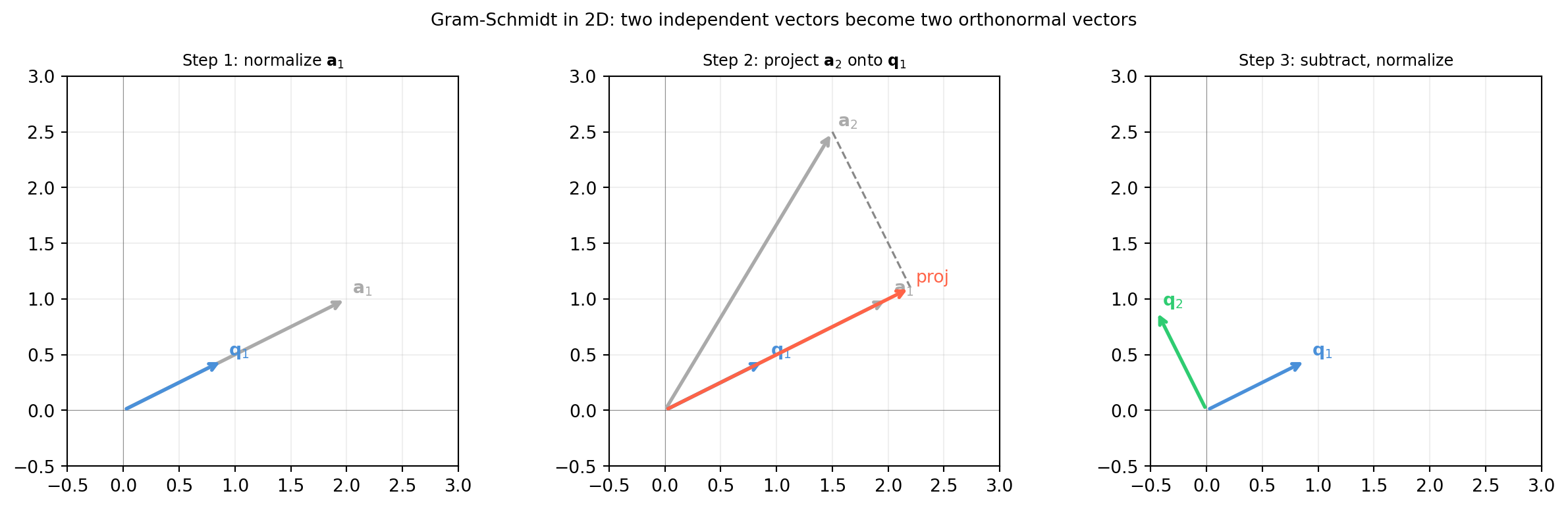
a1 = np.array([2.0, 1.0])         # shape (2,)
a2 = np.array([1.5, 2.5])         # shape (2,)

# Step 1
q1 = a1 / np.linalg.norm(a1)      # shape (2,)

# Step 2
proj = float(q1 @ a2) * q1        # shape (2,) -- projection of a2 onto q1
v2   = a2 - proj                   # shape (2,) -- residual
q2   = v2 / np.linalg.norm(v2)    # shape (2,)

fig, axes = plt.subplots(1, 3, figsize=(13, 4))

data = [
    ('Step 1: normalize $\\mathbf{a}_1$',
     [(a1, '#aaaaaa', r'$\mathbf{a}_1$'),
      (q1, '#4a90d9', r'$\mathbf{q}_1$')], []),
    ('Step 2: project $\\mathbf{a}_2$ onto $\\mathbf{q}_1$',
     [(a1, '#aaaaaa', r'$\mathbf{a}_1$'),
      (a2, '#aaaaaa', r'$\mathbf{a}_2$'),
      (q1, '#4a90d9', r'$\mathbf{q}_1$'),
      (proj, 'tomato', r'proj')],
     [(a2, proj, '--', '#888888')]),
    ('Step 3: subtract, normalize',
     [(q1, '#4a90d9', r'$\mathbf{q}_1$'),
      (q2, '#2ecc71', r'$\mathbf{q}_2$')], []),
]

for ax, (title, vecs, lines) in zip(axes, data):
    ax.set_xlim(-0.5, 3.0)
    ax.set_ylim(-0.5, 3.0)
    ax.set_aspect('equal')
    ax.axhline(0, color='#333333', lw=0.4, alpha=0.5)
    ax.axvline(0, color='#333333', lw=0.4, alpha=0.5)
    ax.grid(True, alpha=0.2)
    ax.set_title(title, fontsize=9)

    for v, c, lbl in vecs:
        ax.annotate('', xy=(v[0], v[1]), xytext=[0, 0],
                    arrowprops=dict(arrowstyle='->', color=c, lw=2))
        ax.text(v[0] + 0.05, v[1] + 0.05, lbl, fontsize=10, color=c)

    for start, end, ls, c in lines:
        ax.plot([start[0], end[0]], [start[1], end[1]], ls=ls, color=c, lw=1.2)

plt.suptitle('Gram-Schmidt in 2D: two independent vectors become two orthonormal vectors',
             fontsize=10)
plt.tight_layout()
plt.show()

print(f"q1 . q2 = {float(q1 @ q2):.2e}  (orthogonal)")
print(f"||q1||  = {np.linalg.norm(q1):.6f},  ||q2|| = {np.linalg.norm(q2):.6f}  (unit)")

q1 . q2 = -1.11e-16  (orthogonal)
||q1||  = 1.000000,  ||q2|| = 1.000000  (unit)

---

16.4.3 Modified Gram-Schmidt: Numerical Stability

Classical Gram-Schmidt (CGS) computes each inner product \(\mathbf{q}_i \cdot \mathbf{a}_j\) using the original column \(\mathbf{a}_j\). In floating-point arithmetic, round-off accumulates across the \(j-1\) subtractions, and the resulting vectors can lose orthogonality on ill-conditioned inputs.

Modified Gram-Schmidt (MGS) reorders the computation: at step \(j\), it subtracts the projections one at a time from the running residual, using the updated vector at each step:

\[\mathbf{v}_j^{(0)} = \mathbf{a}_j, \qquad \mathbf{v}_j^{(i)} = \mathbf{v}_j^{(i-1)} - \bigl(\mathbf{q}_i \cdot \mathbf{v}_j^{(i-1)}\bigr)\mathbf{q}_i, \qquad \mathbf{q}_j = \frac{\mathbf{v}_j^{(j-1)}}{\|\mathbf{v}_j^{(j-1)}\|}.\]

Algebraically identical to CGS, but each subtraction removes the component in the \(\mathbf{q}_i\) direction from the already-reduced vector, so errors do not compound. For production code, Householder QR (§16.5) achieves even higher stability.

import numpy as np

def gram_schmidt_classical(A):
    n, k = A.shape                  # shape (n, k)
    Q = np.zeros((n, k))            # shape (n, k)
    for j in range(k):
        v = A[:, j].copy()          # shape (n,)
        for i in range(j):
            v -= float(Q[:, i] @ A[:, j]) * Q[:, i]
        Q[:, j] = v / np.linalg.norm(v)
    return Q

def gram_schmidt_modified(A):
    n, k = A.shape                  # shape (n, k)
    Q = np.zeros((n, k))            # shape (n, k)
    V = A.astype(float).copy()      # shape (n, k)
    for j in range(k):
        Q[:, j] = V[:, j] / np.linalg.norm(V[:, j])
        for i in range(j + 1, k):
            V[:, i] -= float(Q[:, j] @ V[:, i]) * Q[:, j]
    return Q

def orth_error(Q):
    """Max absolute off-diagonal entry of Q^T Q - I."""
    G = Q.T @ Q - np.eye(Q.shape[1])
    np.fill_diagonal(G, 0.0)
    return float(np.abs(G).max())

# Ill-conditioned test: Hilbert matrix of size 12
n = 12
H_mat = np.array([[1.0 / (i + j + 1) for j in range(n)]
                  for i in range(n)])     # shape (12, 12)

Q_cgs = gram_schmidt_classical(H_mat)
Q_mgs = gram_schmidt_modified(H_mat)

err_cgs = orth_error(Q_cgs)
err_mgs = orth_error(Q_mgs)

print(f"Hilbert matrix, n={n}")
print(f"Classical GS orthogonality error: {err_cgs:.2e}")
print(f"Modified  GS orthogonality error: {err_mgs:.2e}")
print(f"\nMGS is more orthogonal by factor ~{err_cgs / err_mgs:.0f}x")
print("(Householder QR in §16.5 is more stable still.)")

Hilbert matrix, n=12
Classical GS orthogonality error: 1.00e+00
Modified  GS orthogonality error: 2.28e-01

MGS is more orthogonal by factor ~4x
(Householder QR in §16.5 is more stable still.)

---

16.4.4 Exercises

16.4.1 Apply Gram-Schmidt by hand to \(\mathbf{a}_1 = (1, 1, 0)^T\), \(\mathbf{a}_2 = (1, 0, 1)^T\) in \(\mathbb{R}^3\). Produce orthonormal \(\mathbf{q}_1, \mathbf{q}_2\). Verify \(\mathbf{q}_1 \cdot \mathbf{q}_2 = 0\) and \(\|\mathbf{q}_i\| = 1\).

16.4.2 If Gram-Schmidt is applied to a set in which two vectors are identical, what happens at the step corresponding to the duplicate? What does this indicate about the original set?

16.4.3 The Gram-Schmidt process produces \(\mathbf{q}_1, \ldots, \mathbf{q}_k\) from \(\mathbf{a}_1, \ldots, \mathbf{a}_k\). Show that \(\mathbf{q}_j \in \text{span}\{\mathbf{a}_1, \ldots, \mathbf{a}_j\}\) for each \(j\).

16.4.4 Modified GS reorders operations but is algebraically identical to classical GS. To see why it is numerically better, suppose \(\mathbf{q}_1\) is only approximately orthonormal due to round-off. Explain why subtracting from the running residual \(\mathbf{v}_j^{(i)}\) reduces accumulated error compared to subtracting directly from \(\mathbf{a}_j\).

16.5 QR Factorization

Gram-Schmidt applied to the columns of a matrix produces a factorization \(A = QR\): an orthonormal factor \(Q\) and an upper triangular factor \(R\) encoding the Gram-Schmidt coefficients. QR factorization is the workhorse of numerical linear algebra – used in least-squares solving, eigenvalue algorithms, and the computation of orthonormal bases. This section derives the factorization, explains why \(R\) is upper triangular, and describes the Householder algorithm that makes it numerically reliable.

---

16.5.1 Deriving A = QR

Let \(A \in \mathbb{R}^{m \times n}\) have linearly independent columns \(\mathbf{a}_1, \ldots, \mathbf{a}_n\) (so \(m \geq n\)). Gram-Schmidt produces orthonormal \(\mathbf{q}_1, \ldots, \mathbf{q}_n\) with, at each step:

\[\mathbf{a}_j = \sum_{i=1}^{j} r_{ij}\,\mathbf{q}_i, \qquad r_{ij} = \mathbf{q}_i \cdot \mathbf{a}_j \; (i < j), \qquad r_{jj} = \|\mathbf{v}_j\|_2 > 0.\]

Stacking these column-by-column:

\[\boxed{A = QR,} \qquad Q = [\mathbf{q}_1 \;\cdots\; \mathbf{q}_n] \in \mathbb{R}^{m \times n}, \quad R \in \mathbb{R}^{n \times n}.\]

Why is \(R\) upper triangular? \(r_{ij} = \mathbf{q}_i \cdot \mathbf{a}_j\). For \(i > j\), \(\mathbf{q}_i\) was built to be orthogonal to \(\text{span}\{\mathbf{a}_1, \ldots, \mathbf{a}_j\}\), so \(r_{ij} = 0\) – all entries below the diagonal vanish.

Why are diagonal entries positive? \(r_{jj} = \|\mathbf{v}_j\|_2 > 0\) by linear independence. Requiring positive diagonal entries makes the thin QR factorization unique for full-column-rank matrices.

---

16.5.2 Thin vs. Full QR

When \(m > n\) there are two forms:

• Thin QR (reduced): \(Q \in \mathbb{R}^{m \times n}\), \(R \in \mathbb{R}^{n \times n}\). \(Q\) has orthonormal columns, \(Q^T Q = I_n\), but \(QQ^T \neq I_m\). Sufficient for most applications.

• Full QR: \(Q \in \mathbb{R}^{m \times m}\) (square orthogonal), \(R \in \mathbb{R}^{m \times n}\) (padded with zero rows). \(QQ^T = Q^TQ = I_m\).

np.linalg.qr(A, mode='reduced') gives the thin form; mode='complete' gives the full form.

import numpy as np

rng = np.random.default_rng(40)
A = rng.standard_normal((5, 3))    # shape (5, 3)

Q_thin, R_thin = np.linalg.qr(A, mode='reduced')    # Q shape (5, 3), R shape (3, 3)
Q_full, R_full = np.linalg.qr(A, mode='complete')   # Q shape (5, 5), R shape (5, 3)

print("Thin QR:")
print(f"  Q shape: {Q_thin.shape},  R shape: {R_thin.shape}")
print(f"  Q^T Q == I_3: {np.allclose(Q_thin.T @ Q_thin, np.eye(3))}")
print(f"  R upper triangular: {np.allclose(R_thin, np.triu(R_thin))}")
print(f"  A == Q R: {np.allclose(A, Q_thin @ R_thin)}")
d = np.diag(R_thin)
print(f"  Diagonal of R: [{d[0]:.4f}, {d[1]:.4f}, {d[2]:.4f}]")

print("\nFull QR:")
print(f"  Q shape: {Q_full.shape},  R shape: {R_full.shape}")
print(f"  Q Q^T == I_5: {np.allclose(Q_full @ Q_full.T, np.eye(5))}")
print(f"  A == Q R: {np.allclose(A, Q_full @ R_full)}")

Thin QR:
  Q shape: (5, 3),  R shape: (3, 3)
  Q^T Q == I_3: True
  R upper triangular: True
  A == Q R: True
  Diagonal of R: [1.6382, 2.1036, 1.7494]

Full QR:
  Q shape: (5, 5),  R shape: (5, 3)
  Q Q^T == I_5: True
  A == Q R: True

---

16.5.3 Householder Reflections: The Production Algorithm

Gram-Schmidt builds \(Q\) column-by-column, accumulating round-off as noted in §16.4. The numerically preferred approach is Householder reflections, which zero out one column’s subdiagonal entries at a time.

A Householder reflector for \(\mathbf{x} \in \mathbb{R}^m\) is:

\[H = I - 2\frac{\mathbf{v}\mathbf{v}^T}{\mathbf{v}^T\mathbf{v}}, \qquad \mathbf{v} = \mathbf{x} + \text{sign}(x_1)\|\mathbf{x}\|\,\mathbf{e}_1.\]

\(H\) is symmetric (\(H = H^T\)) and orthogonal (\(H^2 = I\)), and \(H\mathbf{x}\) is a scalar multiple of \(\mathbf{e}_1\) – all entries below the first are annihilated. Applying a sequence \(H_n \cdots H_1 A\) progressively zeros out subdiagonal entries column by column until the result is upper triangular: \(H_n \cdots H_1 A = R\), so \(A = H_1 \cdots H_n R = QR\).

Householder QR is backward stable and is the algorithm used in LAPACK’s dgeqrf.

import numpy as np

def householder_reflector(x):
    """Return unit vector v such that H = I - 2vv^T maps x to -sign(x[0])||x|| e_1."""
    v = x.copy().astype(float)     # shape (m,)
    v[0] += np.sign(x[0]) * np.linalg.norm(x)
    norm_v = np.linalg.norm(v)
    if norm_v < 1e-14:
        return v                    # x is already aligned with e_1
    return v / norm_v               # shape (m,)

rng = np.random.default_rng(41)
x = rng.standard_normal(4)         # shape (4,)

v = householder_reflector(x)       # shape (4,)
H = np.eye(4) - 2.0 * np.outer(v, v)   # shape (4, 4)
Hx = H @ x                         # shape (4,)

print(f"x  = {x.round(4)}")
print(f"Hx = {Hx.round(4)}  (should be [+-||x||, 0, 0, 0])")
print(f"||x|| = {np.linalg.norm(x):.4f}")
print(f"\nH symmetric:  {np.allclose(H, H.T)}")
print(f"H orthogonal: {np.allclose(H @ H.T, np.eye(4))}")
print(f"H^2 == I:     {np.allclose(H @ H, np.eye(4))}")

x  = [-1.2317  0.2671 -0.0069  0.5015]
Hx = [ 1.3564 -0.      0.     -0.    ]  (should be [+-||x||, 0, 0, 0])
||x|| = 1.3564

H symmetric:  True
H orthogonal: True
H^2 == I:     True

---

16.5.4 Application: Solving Least Squares via QR

The main application of QR in numerical practice is solving least-squares problems (Chapter 17). For an overdetermined system \(A\mathbf{x} \approx \mathbf{b}\) (\(A\) tall), the normal equations are \(A^T A \hat{\mathbf{x}} = A^T \mathbf{b}\). Using \(A = QR\):

\[A^T A = R^T Q^T Q R = R^T R, \qquad A^T \mathbf{b} = R^T Q^T \mathbf{b}.\]

The normal equations simplify to \(R\hat{\mathbf{x}} = Q^T\mathbf{b}\) (upper triangular back-substitution). This avoids forming \(A^T A\) explicitly, which squares the condition number and loses accuracy when \(A\) is nearly rank-deficient.

import numpy as np

rng = np.random.default_rng(42)
m, n = 20, 4
A = rng.standard_normal((m, n))    # shape (20, 4)
b = rng.standard_normal(m)         # shape (20,)

# Via QR
Q, R = np.linalg.qr(A, mode='reduced')   # Q shape (20, 4), R shape (4, 4)
x_qr = np.linalg.solve(R, Q.T @ b)        # shape (4,)

# Via normal equations (for comparison)
x_ne = np.linalg.solve(A.T @ A, A.T @ b)  # shape (4,)

# NumPy's built-in least squares (Householder internally)
x_ls, _, _, _ = np.linalg.lstsq(A, b, rcond=None)   # shape (4,)

print(f"x (QR):             {x_qr.round(6)}")
print(f"x (normal eqs):     {x_ne.round(6)}")
print(f"x (lstsq):          {x_ls.round(6)}")

resid_qr = np.linalg.norm(A @ x_qr - b)
resid_ne = np.linalg.norm(A @ x_ne - b)
resid_ls = np.linalg.norm(A @ x_ls - b)
print(f"\nResiduals -- QR: {resid_qr:.6f},  NE: {resid_ne:.6f},  lstsq: {resid_ls:.6f}")
print(f"QR vs lstsq diff: {np.linalg.norm(x_qr - x_ls):.2e}")

x (QR):             [ 0.256877 -0.238808  0.008643  0.11457 ]
x (normal eqs):     [ 0.256877 -0.238808  0.008643  0.11457 ]
x (lstsq):          [ 0.256877 -0.238808  0.008643  0.11457 ]

Residuals -- QR: 3.370992,  NE: 3.370992,  lstsq: 3.370992
QR vs lstsq diff: 1.21e-15

---

16.5.5 Exercises

16.5.1 For \(A = \begin{bmatrix}1&1\\1&0\\0&1\end{bmatrix}\), perform Gram-Schmidt by hand to find the QR factorization. Verify \(A = QR\), that \(R\) is upper triangular with positive diagonal, and that \(Q^TQ = I_2\).

16.5.2 For the Householder reflector \(H = I - 2\mathbf{v}\mathbf{v}^T\) with \(\|\mathbf{v}\| = 1\), show: (a) \(H^T = H\), (b) \(H^2 = I\), (c) \(\det(H) = -1\). What does \(\det(H) = -1\) say about \(H\) as an orthogonal map?

16.5.3 Using np.linalg.qr, factor \(A = \begin{bmatrix}2&1&0\\0&2&1\\0&0&2\end{bmatrix}\). What is \(Q\)? What is \(R\)? Explain why a matrix that is already upper triangular with positive diagonal should give \(Q = I_3\) and \(R = A\).

16.5.4 Show that solving via QR (\(R\hat{\mathbf{x}} = Q^T\mathbf{b}\)) is algebraically equivalent to the normal equations (\(A^TA\hat{\mathbf{x}} = A^T\mathbf{b}\)). Why is QR preferred numerically? (Hint: forming \(A^TA\) squares the condition number.)

16.6 Exercises and Solutions

---

16.6.1 Exercise 16.1.2 – Coordinates in an orthonormal basis

Express \(\mathbf{x} = (3, 2, -1)^T\) as a linear combination of \(\mathbf{u}_1 = (1,0,0)^T\), \(\mathbf{u}_2 = (0, 1/\sqrt{2}, 1/\sqrt{2})^T\), \(\mathbf{u}_3 = (0, 1/\sqrt{2}, -1/\sqrt{2})^T\).

import numpy as np

u1 = np.array([1.0, 0.0, 0.0])                       # shape (3,)
u2 = np.array([0.0, 1.0/np.sqrt(2), 1.0/np.sqrt(2)]) # shape (3,)
u3 = np.array([0.0, 1.0/np.sqrt(2), -1.0/np.sqrt(2)])# shape (3,)
U  = np.column_stack([u1, u2, u3])                    # shape (3, 3)

x  = np.array([3.0, 2.0, -1.0])                      # shape (3,)

# Coordinate theorem: c_i = u_i . x
c = U.T @ x                       # shape (3,)
print(f"c1 = u1 . x = {c[0]:.4f}")
print(f"c2 = u2 . x = {c[1]:.4f}")
print(f"c3 = u3 . x = {c[2]:.4f}")

x_rec = U @ c                     # shape (3,)
print(f"\nReconstruction x = c1*u1 + c2*u2 + c3*u3 = {x_rec}")
print(f"Matches x: {np.allclose(x_rec, x)}")

c1 = u1 . x = 3.0000
c2 = u2 . x = 0.7071
c3 = u3 . x = 2.1213

Reconstruction x = c1*u1 + c2*u2 + c3*u3 = [ 3.  2. -1.]
Matches x: True

Solution. By the coordinate theorem \(c_i = \mathbf{u}_i \cdot \mathbf{x}\): \(c_1 = 3\), \(c_2 = (2 + (-1))/\sqrt{2} = 1/\sqrt{2}\), \(c_3 = (2 - (-1))/\sqrt{2} = 3/\sqrt{2}\).

So \(\mathbf{x} = 3\mathbf{u}_1 + \tfrac{1}{\sqrt{2}}\mathbf{u}_2 + \tfrac{3}{\sqrt{2}}\mathbf{u}_3\). No linear system needed – just three dot products.

---

16.6.2 Exercise 16.2.1 – Composing rotation matrices

Compute \(R_\pi R_{-\pi/2}\) and identify the resulting rotation angle.

import numpy as np

def R(theta):
    return np.array([[np.cos(theta), -np.sin(theta)],
                     [np.sin(theta),  np.cos(theta)]])   # shape (2, 2)

M = R(np.pi) @ R(-np.pi / 2)      # shape (2, 2)

print("R_pi @ R_{-pi/2}:")
print(M.round(6))
print(f"\ndet = {np.linalg.det(M):.4f}  (should be 1)")
print(f"M^T M == I: {np.allclose(M.T @ M, np.eye(2))}")

# Identify the angle: cos(theta) = M[0,0]
angle = np.arctan2(M[1, 0], M[0, 0])
print(f"\nResulting angle = {angle:.4f} rad = {np.degrees(angle):.1f} deg")
print(f"Expected: pi + (-pi/2) = pi/2 = {np.pi/2:.4f} rad")

R_pi @ R_{-pi/2}:
[[ 0. -1.]
 [ 1.  0.]]

det = 1.0000  (should be 1)
M^T M == I: True

Resulting angle = 1.5708 rad = 90.0 deg
Expected: pi + (-pi/2) = pi/2 = 1.5708 rad

Solution. Rotation matrices compose by adding angles: \(R_\pi R_{-\pi/2} = R_{\pi - \pi/2} = R_{\pi/2}\).

The result is a \(90°\) counterclockwise rotation: \(\begin{bmatrix}0&-1\\1&0\end{bmatrix}\). Determinant is \(0 \cdot 0 - (-1)(1) = 1\), confirming it is a rotation.

---

16.6.3 Exercise 16.2.3 – Eigenvalue modulus of an orthogonal matrix

Show that if \(Q\) is orthogonal and \(Q\mathbf{v} = \lambda\mathbf{v}\), then \(|\lambda| = 1\).

import numpy as np

rng = np.random.default_rng(50)

# Random orthogonal matrix
A = rng.standard_normal((5, 5))   # shape (5, 5)
Q, _ = np.linalg.qr(A)            # shape (5, 5)

eigvals = np.linalg.eigvals(Q)    # shape (5,) -- may be complex
mods = np.abs(eigvals)            # shape (5,)

print("Eigenvalues of Q:")
for lam, m in zip(eigvals, mods):
    print(f"  {lam.real:+.4f} {lam.imag:+.4f}i   |lambda| = {m:.6f}")

print(f"\nAll |lambda| == 1: {np.allclose(mods, 1.0)}")

Eigenvalues of Q:
  +1.0000 +0.0000i   |lambda| = 1.000000
  -0.0674 +0.9977i   |lambda| = 1.000000
  -0.0674 -0.9977i   |lambda| = 1.000000
  -0.9662 +0.2578i   |lambda| = 1.000000
  -0.9662 -0.2578i   |lambda| = 1.000000

All |lambda| == 1: True

Solution. Let \(Q\mathbf{v} = \lambda\mathbf{v}\) with \(\mathbf{v} \neq \mathbf{0}\). Apply the isometry property to \(\mathbf{v}\):

\[\|\mathbf{v}\|_2 = \|Q\mathbf{v}\|_2 = \|\lambda\mathbf{v}\|_2 = |\lambda|\,\|\mathbf{v}\|_2.\]

Dividing by \(\|\mathbf{v}\|_2 > 0\) gives \(|\lambda| = 1\). Eigenvalues of real orthogonal matrices are either \(\pm 1\) (for real eigenvectors) or complex conjugate pairs on the unit circle \(e^{\pm i\theta}\) (for complex eigenvectors).

---

16.6.4 Exercise 16.3.1 – Orthogonal complement in R^3

Let \(W = \text{span}\{(1,1,0)^T\}\) in \(\mathbb{R}^3\). Find a basis for \(W^\perp\).

import numpy as np

w = np.array([1.0, 1.0, 0.0])     # shape (3,) -- generator of W

# W^perp = null space of w^T
# Solve w . v = 0: v_1 + v_2 = 0 -- two free variables
# Basis: v_1 = (1,-1,0)^T, v_2 = (0,0,1)^T
v1 = np.array([1.0, -1.0, 0.0])   # shape (3,)
v2 = np.array([0.0,  0.0, 1.0])   # shape (3,)

print(f"w . v1 = {float(w @ v1)}  (should be 0)")
print(f"w . v2 = {float(w @ v2)}  (should be 0)")
print(f"v1 . v2 = {float(v1 @ v2)}  (they happen to be orthogonal)")

print(f"\ndim(W)       = 1")
print(f"dim(W^perp)  = 2  (basis: v1, v2)")
print(f"dim(W) + dim(W^perp) = 3 = n  (dimension theorem)")

w . v1 = 0.0  (should be 0)
w . v2 = 0.0  (should be 0)
v1 . v2 = 0.0  (they happen to be orthogonal)

dim(W)       = 1
dim(W^perp)  = 2  (basis: v1, v2)
dim(W) + dim(W^perp) = 3 = n  (dimension theorem)

Solution. \(W^\perp\) consists of all \(\mathbf{v} = (v_1, v_2, v_3)^T\) with \(\mathbf{w} \cdot \mathbf{v} = v_1 + v_2 = 0\). Setting \(v_2 = -v_1\) and \(v_3\) free:

\[W^\perp = \text{span}\left\{(1,-1,0)^T,\; (0,0,1)^T\right\}.\]

The dimension theorem gives \(1 + 2 = 3\) as expected.

---

16.6.5 Exercise 16.4.1 – Gram-Schmidt by hand

Apply Gram-Schmidt to \(\mathbf{a}_1 = (1,1,0)^T\), \(\mathbf{a}_2 = (1,0,1)^T\).

import numpy as np

a1 = np.array([1.0, 1.0, 0.0])    # shape (3,)
a2 = np.array([1.0, 0.0, 1.0])    # shape (3,)

# Step 1: normalize a1
q1 = a1 / np.linalg.norm(a1)      # shape (3,)

# Step 2: subtract projection of a2 onto q1, then normalize
v2 = a2 - float(q1 @ a2) * q1     # shape (3,)
q2 = v2 / np.linalg.norm(v2)      # shape (3,)

print(f"q1 = {q1.round(6)}")
print(f"q2 = {q2.round(6)}")
print(f"\nq1 . q2 = {float(q1 @ q2):.2e}  (orthogonal)")
print(f"||q1||  = {np.linalg.norm(q1):.6f}  (unit)")
print(f"||q2||  = {np.linalg.norm(q2):.6f}  (unit)")

q1 = [0.707107 0.707107 0.      ]
q2 = [ 0.408248 -0.408248  0.816497]

q1 . q2 = 1.11e-16  (orthogonal)
||q1||  = 1.000000  (unit)
||q2||  = 1.000000  (unit)

Solution. Step 1: \(\mathbf{q}_1 = \mathbf{a}_1/\|\mathbf{a}_1\| = (1,1,0)^T/\sqrt{2}\).

Step 2: \(r_{12} = \mathbf{q}_1 \cdot \mathbf{a}_2 = (1 \cdot 1 + 1 \cdot 0 + 0 \cdot 1)/\sqrt{2} = 1/\sqrt{2}\). Residual: \(\mathbf{v}_2 = \mathbf{a}_2 - \tfrac{1}{\sqrt{2}}\mathbf{q}_1 = (1,0,1)^T - \tfrac{1}{2}(1,1,0)^T = (1/2, -1/2, 1)^T\). Normalized: \(\mathbf{q}_2 = \mathbf{v}_2/\|\mathbf{v}_2\|\) with \(\|\mathbf{v}_2\| = \sqrt{1/4 + 1/4 + 1} = \sqrt{3/2}\).

---

16.6.6 Exercise 16.4.3 – Gram-Schmidt span preservation

Show that \(\mathbf{q}_j \in \text{span}\{\mathbf{a}_1, \ldots, \mathbf{a}_j\}\) for each \(j\).

Solution. By induction. Base case \(j=1\): \(\mathbf{q}_1 = \mathbf{a}_1/\|\mathbf{a}_1\|\), which is a scalar multiple of \(\mathbf{a}_1 \in \text{span}\{\mathbf{a}_1\}\). \(\checkmark\)

Inductive step: assume \(\mathbf{q}_i \in \text{span}\{\mathbf{a}_1, \ldots, \mathbf{a}_i\}\) for all \(i < j\). Then each projection \((\mathbf{q}_i \cdot \mathbf{a}_j)\mathbf{q}_i\) is in \(\text{span}\{\mathbf{a}_1, \ldots, \mathbf{a}_{j-1}\}\) by hypothesis. Therefore

\[\mathbf{v}_j = \mathbf{a}_j - \sum_{i<j}(\mathbf{q}_i \cdot \mathbf{a}_j)\mathbf{q}_i \;\in\; \text{span}\{\mathbf{a}_1, \ldots, \mathbf{a}_j\},\]

and \(\mathbf{q}_j = \mathbf{v}_j/\|\mathbf{v}_j\|\) inherits this membership. Combined with the symmetric argument (each \(\mathbf{a}_j\) can be reconstructed from \(\mathbf{q}_1, \ldots, \mathbf{q}_j\)), the two spans are equal. \(\square\)

---

16.6.7 Exercise 16.5.1 – QR factorization by hand

Factor \(A = \begin{bmatrix}1&1\\1&0\\0&1\end{bmatrix}\) by Gram-Schmidt.

import numpy as np

A = np.array([[1.0, 1.0],
              [1.0, 0.0],
              [0.0, 1.0]])          # shape (3, 2)

a1 = A[:, 0]                        # shape (3,)
a2 = A[:, 1]                        # shape (3,)

# Step 1
q1 = a1 / np.linalg.norm(a1)       # shape (3,)
r11 = np.linalg.norm(a1)

# Step 2
r12 = float(q1 @ a2)
v2  = a2 - r12 * q1                 # shape (3,)
r22 = np.linalg.norm(v2)
q2  = v2 / r22                      # shape (3,)

Q = np.column_stack([q1, q2])       # shape (3, 2)
R = np.array([[r11, r12],
              [0.0, r22]])           # shape (2, 2)

print("Q:")
print(Q.round(6))
print("\nR:")
print(R.round(6))
print(f"\nA == Q R: {np.allclose(A, Q @ R)}")
print(f"Q^T Q == I_2: {np.allclose(Q.T @ Q, np.eye(2))}")
print(f"R upper triangular, positive diagonal: r11={r11:.4f}, r22={r22:.4f}")

Q:
[[ 0.707107  0.408248]
 [ 0.707107 -0.408248]
 [ 0.        0.816497]]

R:
[[1.414214 0.707107]
 [0.       1.224745]]

A == Q R: True
Q^T Q == I_2: True
R upper triangular, positive diagonal: r11=1.4142, r22=1.2247

Solution. \(\mathbf{q}_1 = (1,1,0)^T/\sqrt{2}\), \(r_{11} = \sqrt{2}\). \(r_{12} = \mathbf{q}_1 \cdot \mathbf{a}_2 = 1/\sqrt{2}\). \(\mathbf{v}_2 = (1,0,1)^T - \tfrac{1}{2}(1,1,0)^T = (1/2, -1/2, 1)^T\), \(r_{22} = \sqrt{3/2}\), \(\mathbf{q}_2 = \mathbf{v}_2/r_{22}\).

\[R = \begin{bmatrix}\sqrt{2} & 1/\sqrt{2} \\ 0 & \sqrt{3/2}\end{bmatrix}.\]

Both diagonal entries are positive, confirming uniqueness.

---

16.6.8 Exercise 16.5.3 – QR of an upper triangular matrix

import numpy as np

A = np.array([[2.0, 1.0, 0.0],
              [0.0, 2.0, 1.0],
              [0.0, 0.0, 2.0]])    # shape (3, 3)

Q, R = np.linalg.qr(A, mode='reduced')   # Q shape (3, 3), R shape (3, 3)

print("Q:")
print(Q.round(6))
print("\nR:")
print(R.round(6))
print(f"\nQ == I_3: {np.allclose(Q, np.eye(3))}")
print(f"R == A:   {np.allclose(R, A)}")
print(f"\ndiag(R): {np.diag(R).round(4)}  (all positive)")

Q:
[[ 1.  0.  0.]
 [-0.  1.  0.]
 [-0. -0.  1.]]

R:
[[2. 1. 0.]
 [0. 2. 1.]
 [0. 0. 2.]]

Q == I_3: True
R == A:   True

diag(R): [2. 2. 2.]  (all positive)

Solution. If \(A\) is already upper triangular with positive diagonal entries, then its columns satisfy the Gram-Schmidt conditions: \(\mathbf{a}_1\) is already along \(\mathbf{e}_1\)’s direction (no component outside span), and each \(\mathbf{a}_j\) has no component along \(\mathbf{a}_{j+1}, \ldots\) (upper triangular means the previous \(\mathbf{q}_i\) projections are already encoded). The algorithm produces \(\mathbf{q}_j = \mathbf{e}_j\) normalized, which for a full-rank triangular matrix collapses to \(Q = I_3\), \(R = A\). The positive diagonal requirement is met because the diagonal entries of \(A\) are \(2 > 0\).