19 Covariance, Statistical Geometry, and the Matrix Square Root

19.1 Mean-Centering and the Data Matrix

A dataset of \(n\) observations, each with \(p\) measured features, is arranged into an \(n \times p\) matrix:

\[X = \begin{bmatrix} \mathbf{x}_1^T \\ \vdots \\ \mathbf{x}_n^T \end{bmatrix} \in \mathbb{R}^{n \times p},\]

where row \(\mathbf{x}_i^T \in \mathbb{R}^p\) is one observation. Almost every operation in statistical geometry – covariance, PCA, Mahalanobis distance – begins with the same preparatory step: mean-centering.

19.1.1 Why Center?

The sample mean of each feature \(j\) is

\[\bar{x}_j = \frac{1}{n}\sum_{i=1}^n X_{ij}.\]

Collected into a row vector \(\bar{\mathbf{x}}^T \in \mathbb{R}^p\), the centered matrix is

\[\boxed{\tilde{X} = X - \mathbf{1}_n \bar{\mathbf{x}}^T,}\]

where \(\mathbf{1}_n\) is the \(n\)-vector of ones. Row \(i\) of \(\tilde{X}\) is \(\tilde{\mathbf{x}}_i = \mathbf{x}_i - \bar{\mathbf{x}}\), the deviation from the mean.

The column sums of \(\tilde{X}\) are exactly zero: \(\tilde{X}^T \mathbf{1}_n = \mathbf{0}\).

What if you skip centering?

If \(X\) is not centered, then \(\frac{1}{n-1}X^TX\) is the second-moment matrix, not the covariance matrix. The two coincide only when \(\bar{\mathbf{x}} = \mathbf{0}\). In practice, skipping the centering step means your “covariance” mixes genuine spread with the offset of the cloud from the origin – a common source of incorrect PCA results.

19.1.2 Centering as a Projection

Centering is a linear map. Define the centering matrix

\[H = I_n - \frac{1}{n}\mathbf{1}_n\mathbf{1}_n^T \in \mathbb{R}^{n \times n}.\]

Then \(\tilde{X} = HX\). \(H\) is symmetric and idempotent (\(H^2 = H\)), so it is an orthogonal projection onto the subspace orthogonal to \(\mathbf{1}_n\). This geometric view matters: centering removes the component of each column of \(X\) that is constant across observations.

19.1.3 Numerical Example

import numpy as np

rng = np.random.default_rng(191)

# Simulate n=6 observations, p=3 features (height cm, weight kg, age yr)
X = np.array([[170, 65, 28],   # shape (6, 3)
              [182, 80, 35],
              [158, 55, 22],
              [175, 72, 41],
              [165, 60, 30],
              [190, 90, 45]], dtype=float)

# Sample mean (one per feature)
x_bar = X.mean(axis=0)   # shape (3,)
print("Sample means:", x_bar.round(4))

# Centered matrix
X_tilde = X - x_bar      # shape (6, 3)  -- broadcasting subtracts row-wise
print("\nCentered matrix X_tilde:")
print(X_tilde.round(4))

# Column sums must be zero (up to floating-point rounding)
print("\nColumn sums of X_tilde:", X_tilde.sum(axis=0).round(10))

# Equivalently, using the centering matrix H
n = X.shape[0]                                         # n = 6
H = np.eye(n) - np.ones((n, n)) / n                   # shape (6, 6)
X_tilde_H = H @ X                                      # shape (6, 3)
print("\n||X_tilde - H @ X||_F =", np.linalg.norm(X_tilde - X_tilde_H).round(12))

Sample means: [173.3333  70.3333  33.5   ]

Centered matrix X_tilde:
[[ -3.3333  -5.3333  -5.5   ]
 [  8.6667   9.6667   1.5   ]
 [-15.3333 -15.3333 -11.5   ]
 [  1.6667   1.6667   7.5   ]
 [ -8.3333 -10.3333  -3.5   ]
 [ 16.6667  19.6667  11.5   ]]

Column sums of X_tilde: [-0.  0.  0.]

||X_tilde - H @ X||_F = 0.0

19.1.4 Visualizing the Effect of Centering

import numpy as np
import matplotlib.pyplot as plt

rng = np.random.default_rng(1912)

# 2-D dataset with a non-zero mean for clarity
mean_true = np.array([4.0, 7.0])       # shape (2,)
cov_true  = np.array([[2.0, 1.2],      # shape (2, 2)
                       [1.2, 1.5]])
n = 120
L = np.linalg.cholesky(cov_true)       # shape (2, 2)
X = rng.standard_normal((n, 2)) @ L.T + mean_true  # shape (120, 2)

x_bar = X.mean(axis=0)    # shape (2,)
X_tilde = X - x_bar       # shape (120, 2)

fig, axes = plt.subplots(1, 2, figsize=(11, 4.5))

for ax, data, title, col in zip(
        axes,
        [X, X_tilde],
        ['Original $X$', 'Centered $\\tilde{X}$'],
        ['#4a90d9', '#2ecc71']):
    ax.scatter(data[:, 0], data[:, 1], s=20, color=col, alpha=0.6)
    ax.axhline(0, color='#333333', lw=0.4, alpha=0.5)
    ax.axvline(0, color='#333333', lw=0.4, alpha=0.5)
    cx, cy = data.mean(axis=0)
    ax.scatter([cx], [cy], s=80, color='tomato', zorder=5, label='mean')
    ax.set_title(title, fontsize=12)
    ax.legend(fontsize=9)
    ax.grid(alpha=0.2)
    ax.set_aspect('equal')

fig.suptitle('Effect of mean-centering', fontsize=13)
fig.tight_layout()
plt.savefig('ch19-covariance/fig-centering.png', dpi=150, bbox_inches='tight')
plt.show()

print(f"Mean before centering: {X.mean(axis=0).round(4)}")
print(f"Mean after centering:  {X_tilde.mean(axis=0).round(10)}")

Mean before centering: [4.3351 7.2594]
Mean after centering:  [ 0. -0.]

19.1.5 Exercises

19.1.1 The centering matrix \(H = I_n - \frac{1}{n}\mathbf{1}\mathbf{1}^T\). Verify that \(H^2 = H\) and that \(H\mathbf{1} = \mathbf{0}\). What does idempotency mean geometrically?

19.1.2 Show that centering is invariant to an overall additive shift: if you replace \(X\) with \(X + \mathbf{1}_n \mathbf{c}^T\) (adding the same constant vector \(\mathbf{c}\) to every row), the centered result \(\tilde{X}\) is unchanged.

19.1.3 Suppose you center the columns but not the rows. What does the row sum \(\tilde{X}\mathbf{1}_p\) look like? Is row-centering ever useful? (Hint: think about double-centering in collaborative filtering.)

19.1.4 If \(X\) already has zero mean (a previous step ensured this), prove that \(\frac{1}{n-1}X^TX = \frac{1}{n}X^TX\) in the limit as \(n \to \infty\). Why do we use \(n-1\) instead of \(n\) for finite samples?

19.2 The Covariance Matrix

Given the centered data matrix \(\tilde{X} \in \mathbb{R}^{n \times p}\) (§19.1), the sample covariance matrix is

\[\boxed{\Sigma = \frac{1}{n-1}\tilde{X}^T\tilde{X} \in \mathbb{R}^{p \times p}.}\]

Entry \((j,k)\) of \(\Sigma\) is the sample covariance between features \(j\) and \(k\):

\[\Sigma_{jk} = \frac{1}{n-1}\sum_{i=1}^n \tilde{X}_{ij}\tilde{X}_{ik}.\]

The diagonal entries \(\Sigma_{jj} = s_j^2\) are the sample variances; the off-diagonal entries measure linear co-variation.

19.2.1 Structure: Symmetric PSD

\(\Sigma\) is symmetric by construction: \(\Sigma^T = \frac{1}{n-1}(\tilde{X}^T\tilde{X})^T = \Sigma\).

\(\Sigma\) is positive semidefinite: for any \(\mathbf{v} \in \mathbb{R}^p\),

\[\mathbf{v}^T \Sigma \mathbf{v} = \frac{1}{n-1}\|\tilde{X}\mathbf{v}\|_2^2 \ge 0.\]

It is positive definite (all eigenvalues strictly positive) when \(\tilde{X}\) has full column rank, i.e., \(n > p\) and no feature is a linear combination of the others.

19.2.2 Eigenstructure as the Data Ellipsoid

The spectral decomposition of \(\Sigma\) is

\[\Sigma = Q \Lambda Q^T, \qquad \Lambda = \text{diag}(\lambda_1, \ldots, \lambda_p), \quad \lambda_1 \ge \cdots \ge \lambda_p \ge 0,\]

where \(Q \in \mathbb{R}^{p \times p}\) is orthogonal (eigenvectors as columns).

Geometric interpretation:

Eigenvectors \(\mathbf{q}_1, \ldots, \mathbf{q}_p\) are the principal axes of the data cloud – the directions of greatest (then second greatest, etc.) spread.
Eigenvalues \(\lambda_j\) are the variances along those axes: the cloud extends \(\sqrt{\lambda_j}\) standard deviations along \(\mathbf{q}_j\).
The iso-density contour \(\{\mathbf{x} : \mathbf{x}^T \Sigma^{-1} \mathbf{x} = c^2\}\) (when \(\bar{\mathbf{x}} = \mathbf{0}\)) is an ellipsoid with semi-axes \(c\sqrt{\lambda_j}\) along \(\mathbf{q}_j\).

This ellipsoid is the fingerprint of the distribution’s shape.

19.2.3 Connection to SVD

The thin SVD of the centered matrix \(\tilde{X} = U S V^T\) gives immediately:

\[\Sigma = \frac{1}{n-1}\tilde{X}^T\tilde{X} = \frac{1}{n-1}V S^2 V^T.\]

So: - Eigenvectors of \(\Sigma\) = right singular vectors \(V\) of \(\tilde{X}\). - Eigenvalues of \(\Sigma\) = \(\sigma_i^2/(n-1)\) where \(\sigma_i\) are singular values of \(\tilde{X}\).

This is the linear-algebraic core of PCA.

19.2.4 Numerical Example

import numpy as np

rng = np.random.default_rng(192)

# Simulate n=200 observations, p=2 features with known covariance
mean_true = np.array([3.0, 5.0])     # shape (2,)
cov_true  = np.array([[4.0, 2.4],    # shape (2, 2)
                       [2.4, 2.0]])
n, p = 200, 2

# Generate data via Cholesky
L = np.linalg.cholesky(cov_true)     # shape (2, 2)
X = rng.standard_normal((n, p)) @ L.T + mean_true  # shape (200, 2)

# Mean-center
x_bar = X.mean(axis=0)              # shape (2,)
X_tilde = X - x_bar                 # shape (200, 2)

# Sample covariance
Sigma_hat = X_tilde.T @ X_tilde / (n - 1)   # shape (2, 2)
print("True covariance:\n", cov_true)
print("\nSample covariance:\n", Sigma_hat.round(4))

# Eigendecomposition
lam, Q = np.linalg.eigh(Sigma_hat)  # eigenvalues ascending
idx = np.argsort(lam)[::-1]         # sort descending
lam = lam[idx]                       # shape (2,)
Q   = Q[:, idx]                      # shape (2, 2) -- columns are eigenvectors
print(f"\nEigenvalues:  lambda_1 = {lam[0]:.4f},  lambda_2 = {lam[1]:.4f}")
print("Eigenvectors (columns of Q):\n", Q.round(4))
print(f"\nStd dev along PC1: sqrt(lambda_1) = {np.sqrt(lam[0]):.4f}")
print(f"Std dev along PC2: sqrt(lambda_2) = {np.sqrt(lam[1]):.4f}")

# Cross-check via SVD of X_tilde
U_svd, s_svd, Vt_svd = np.linalg.svd(X_tilde, full_matrices=False)
# shape (200,2), (2,), (2,2)
lam_from_svd = s_svd**2 / (n - 1)   # shape (2,)
print(f"\nEigenvalues from SVD: {lam_from_svd.round(4)}")

True covariance:
 [[4.  2.4]
 [2.4 2. ]]

Sample covariance:
 [[4.3457 2.62  ]
 [2.62   2.0833]]

Eigenvalues:  lambda_1 = 6.0683,  lambda_2 = 0.3607
Eigenvectors (columns of Q):
 [[-0.8356  0.5494]
 [-0.5494 -0.8356]]

Std dev along PC1: sqrt(lambda_1) = 2.4634
Std dev along PC2: sqrt(lambda_2) = 0.6006

Eigenvalues from SVD: [6.0683 0.3607]

19.2.5 Visualizing the Covariance Ellipse

import numpy as np
import matplotlib.pyplot as plt
from matplotlib.patches import Ellipse

rng = np.random.default_rng(1921)

mean_true = np.array([0.0, 0.0])
cov_true  = np.array([[4.0, 2.4],
                       [2.4, 2.0]])
n = 300
L = np.linalg.cholesky(cov_true)        # shape (2, 2)
X = rng.standard_normal((n, 2)) @ L.T   # shape (300, 2)

Sigma_hat = X.T @ X / (n - 1)           # shape (2, 2) -- already zero-mean
lam, Q = np.linalg.eigh(Sigma_hat)
idx = np.argsort(lam)[::-1]
lam = lam[idx];  Q = Q[:, idx]          # shape (2,), (2, 2)

fig, ax = plt.subplots(figsize=(6, 6))
ax.scatter(X[:, 0], X[:, 1], s=8, color='#4a90d9', alpha=0.35, label='data')

# Draw 1-, 2-, 3-sigma ellipses
for n_sig, alpha_ell, lbl in [(1, 0.75, '1$\\sigma$'), (2, 0.5, '2$\\sigma$'), (3, 0.3, '3$\\sigma$')]:
    width  = 2 * n_sig * np.sqrt(lam[0])
    height = 2 * n_sig * np.sqrt(lam[1])
    angle  = np.degrees(np.arctan2(Q[1, 0], Q[0, 0]))
    ell = Ellipse(xy=(0, 0), width=width, height=height, angle=angle,
                  edgecolor='tomato', facecolor='none', lw=1.5, alpha=alpha_ell, label=lbl)
    ax.add_patch(ell)

# Draw principal axes
scale = 2.5
for j in range(2):
    v = Q[:, j] * np.sqrt(lam[j]) * scale
    ax.annotate('', xy=v, xytext=[0, 0],
                arrowprops=dict(arrowstyle='->', color='#2ecc71', lw=2.2))
    ax.annotate('', xy=-v, xytext=[0, 0],
                arrowprops=dict(arrowstyle='->', color='#2ecc71', lw=2.2))
    ax.text(v[0] + 0.15, v[1] + 0.15,
            f'$\\mathbf{{q}}_{j+1}$, $\\lambda_{j+1}={lam[j]:.2f}$',
            fontsize=10, color='#2ecc71')

ax.axhline(0, color='#333333', lw=0.4, alpha=0.5)
ax.axvline(0, color='#333333', lw=0.4, alpha=0.5)
ax.set_aspect('equal')
ax.legend(fontsize=9, loc='upper left')
ax.set_title('Covariance ellipse: principal axes and $\\sigma$ contours', fontsize=12)
ax.grid(alpha=0.2)
fig.tight_layout()
plt.savefig('ch19-covariance/fig-cov-ellipse.png', dpi=150, bbox_inches='tight')
plt.show()
print(f"Ellipse angle from x-axis: {np.degrees(np.arctan2(Q[1,0], Q[0,0])):.2f} deg")

Ellipse angle from x-axis: -145.93 deg

19.2.6 Exercises

19.2.1 Show that \(\Sigma = \frac{1}{n-1}\tilde{X}^T\tilde{X}\) is equivalent to \(\Sigma_{jk} = \frac{1}{n-1}\sum_i \tilde{X}_{ij}\tilde{X}_{ik}\) by expanding the matrix product entry-by-entry.

19.2.2 Prove that \(\mathbf{v}^T\Sigma\mathbf{v} \ge 0\) for all \(\mathbf{v}\). When does equality hold?

19.2.3 If features \(j\) and \(k\) are uncorrelated in the sample (\(\Sigma_{jk} = 0\)), what does this say geometrically about the covariance ellipse? Is it possible for two features to be uncorrelated yet not independent?

19.2.4 The correlation matrix is \(R_{jk} = \Sigma_{jk}/\sqrt{\Sigma_{jj}\Sigma_{kk}}\). Show that \(R = D^{-1/2}\Sigma D^{-1/2}\) where \(D = \text{diag}(\Sigma_{11},\ldots,\Sigma_{pp})\). Why are all diagonal entries of \(R\) equal to 1?

19.3 The Multivariate Gaussian and Its Geometry

The multivariate Gaussian \(\mathbf{x} \sim \mathcal{N}(\boldsymbol{\mu}, \Sigma)\) has density

\[\boxed{p(\mathbf{x}) = \frac{1}{(2\pi)^{p/2}|\Sigma|^{1/2}} \exp\!\left(-\tfrac{1}{2}(\mathbf{x}-\boldsymbol{\mu})^T\Sigma^{-1}(\mathbf{x}-\boldsymbol{\mu})\right),}\]

where \(\boldsymbol{\mu} \in \mathbb{R}^p\) is the mean and \(\Sigma \in \mathbb{R}^{p \times p}\) is positive definite. Every term in the formula has a linear-algebraic identity: \(|\Sigma|\) is the determinant (volume scaling), and the exponent is a quadratic form in \(\Sigma^{-1}\).

19.3.1 Iso-Density Contours Are Ellipsoids

\(p(\mathbf{x}) = c\) iff the exponent is constant:

\[(\mathbf{x} - \boldsymbol{\mu})^T \Sigma^{-1} (\mathbf{x} - \boldsymbol{\mu}) = k^2.\]

This is the equation of an ellipsoid centered at \(\boldsymbol{\mu}\). Using the spectral decomposition \(\Sigma = Q\Lambda Q^T\), so \(\Sigma^{-1} = Q\Lambda^{-1}Q^T\):

\[\|\Lambda^{-1/2}Q^T(\mathbf{x} - \boldsymbol{\mu})\|_2^2 = k^2.\]

Let \(\mathbf{z} = \Lambda^{-1/2}Q^T(\mathbf{x}-\boldsymbol{\mu})\); the contour is the sphere \(\|\mathbf{z}\|=k\) in the whitened coordinate system. Back in original coordinates, the semi-axes of the ellipsoid are \(k\sqrt{\lambda_j}\) along \(\mathbf{q}_j\).

Three interpretations of \(k\): - \(k=1\): the 1-sigma ellipsoid, contains \(\approx 39\%\) of Gaussian mass in 2-D (vs. \(68\%\) for the univariate 1-sigma interval). - \(k^2 \sim \chi^2_p\): for a \(p\)-dimensional Gaussian, the squared Mahalanobis distance follows a chi-squared distribution with \(p\) degrees of freedom. - \(k = \sqrt{\chi^2_{p,0.95}}\): the \(95\%\) confidence ellipsoid for \(\boldsymbol{\mu}\).

19.3.2 Marginals and Conditionals Stay Gaussian

Two key closure properties that follow from the quadratic-form structure:

Marginals. If \(\mathbf{x} = [\mathbf{x}_A^T, \mathbf{x}_B^T]^T \sim \mathcal{N}(\boldsymbol{\mu}, \Sigma)\) with block partition \(\Sigma = \begin{bmatrix}\Sigma_{AA} & \Sigma_{AB} \\ \Sigma_{BA} & \Sigma_{BB}\end{bmatrix}\), then \(\mathbf{x}_A \sim \mathcal{N}(\boldsymbol{\mu}_A, \Sigma_{AA})\). Marginalizing out \(\mathbf{x}_B\) leaves the upper-left block – no other distribution shares this property so cleanly.

Conditionals. Given \(\mathbf{x}_B = \mathbf{b}\):

\[\mathbf{x}_A \mid \mathbf{x}_B = \mathbf{b} \;\sim\; \mathcal{N}\!\left( \boldsymbol{\mu}_A + \Sigma_{AB}\Sigma_{BB}^{-1}(\mathbf{b} - \boldsymbol{\mu}_B),\; \Sigma_{AA} - \Sigma_{AB}\Sigma_{BB}^{-1}\Sigma_{BA}\right).\]

The conditional mean is linear in \(\mathbf{b}\); the conditional covariance \(\Sigma_{AA} - \Sigma_{AB}\Sigma_{BB}^{-1}\Sigma_{BA}\) is the Schur complement (always PSD, always \(\le \Sigma_{AA}\) – observing \(\mathbf{x}_B\) can only reduce uncertainty).

These two facts underlie Kalman filtering, Gaussian process regression, and Bayesian linear models.

19.3.3 Numerical Example

import numpy as np
from scipy.stats import chi2

rng = np.random.default_rng(193)

mu    = np.array([2.0, 3.0])         # shape (2,)
Sigma = np.array([[3.0, 1.8],        # shape (2, 2)
                  [1.8, 2.0]])
n = 500
L = np.linalg.cholesky(Sigma)        # shape (2, 2)
X = rng.standard_normal((n, 2)) @ L.T + mu  # shape (500, 2)

# Compute Mahalanobis distance squared for each sample
Sigma_inv = np.linalg.inv(Sigma)     # shape (2, 2)
d_centered = X - mu                  # shape (500, 2)
maha2 = np.einsum('ni,ij,nj->n', d_centered, Sigma_inv, d_centered)  # shape (500,)

# Chi-squared threshold for 95% ellipse (p=2 -> chi2_2)
thresh_95 = chi2.ppf(0.95, df=2)
frac_inside = (maha2 <= thresh_95).mean()
print(f"Chi-squared 95% threshold (df=2): {thresh_95:.4f}")
print(f"Fraction of samples inside 95% ellipse: {frac_inside:.4f}  (expect ~0.95)")

# Conditional distribution: given x_B = 4.0, what is p(x_A)?
x_B = 4.0
mu_cond   = mu[0] + Sigma[0,1] / Sigma[1,1] * (x_B - mu[1])
var_cond  = Sigma[0,0] - Sigma[0,1]**2 / Sigma[1,1]
print(f"\nConditional x_A | x_B = {x_B}:")
print(f"  Mean:     {mu_cond:.4f}")
print(f"  Variance: {var_cond:.4f}  (unconditional was {Sigma[0,0]:.4f})")

Chi-squared 95% threshold (df=2): 5.9915
Fraction of samples inside 95% ellipse: 0.9420  (expect ~0.95)

Conditional x_A | x_B = 4.0:
  Mean:     2.9000
  Variance: 1.3800  (unconditional was 3.0000)

19.3.4 Visualization: Iso-density Contours

import numpy as np
import matplotlib.pyplot as plt
from matplotlib.patches import Ellipse
from scipy.stats import chi2

rng = np.random.default_rng(1930)

mu    = np.array([2.0, 3.0])
Sigma = np.array([[3.0, 1.8],
                  [1.8, 2.0]])
n = 400
L = np.linalg.cholesky(Sigma)
X = rng.standard_normal((n, 2)) @ L.T + mu   # shape (400, 2)

lam, Q = np.linalg.eigh(Sigma)
idx = np.argsort(lam)[::-1]
lam = lam[idx];  Q = Q[:, idx]               # shape (2,), (2, 2)
angle = np.degrees(np.arctan2(Q[1, 0], Q[0, 0]))

fig, ax = plt.subplots(figsize=(6.5, 6))
ax.scatter(X[:, 0], X[:, 1], s=8, color='#4a90d9', alpha=0.35, label='samples')

# Chi-squared contours at 50%, 90%, 99%
levels = [(0.50, '#2ecc71', '50%'), (0.90, 'tomato', '90%'), (0.99, '#e67e22', '99%')]
for prob, color, label in levels:
    k2 = chi2.ppf(prob, df=2)          # chi-squared quantile
    k  = np.sqrt(k2)
    width  = 2 * k * np.sqrt(lam[0])
    height = 2 * k * np.sqrt(lam[1])
    ell = Ellipse(xy=mu, width=width, height=height, angle=angle,
                  edgecolor=color, facecolor='none', lw=2, label=f'{label} contour')
    ax.add_patch(ell)

ax.scatter(*mu, s=80, color='tomato', zorder=5, label='$\\mu$')
ax.set_aspect('equal')
ax.legend(fontsize=9)
ax.set_title('Multivariate Gaussian: iso-density ellipses', fontsize=12)
ax.grid(alpha=0.2)
fig.tight_layout()
plt.savefig('ch19-covariance/fig-gauss-contours.png', dpi=150, bbox_inches='tight')
plt.show()

19.3.5 Exercises

19.3.1 In 1-D, the “1-sigma interval” \([\mu - \sigma, \mu + \sigma]\) contains \(68\%\) of the Gaussian mass. In 2-D, compute the fraction of mass inside the 1-sigma ellipsoid (i.e., \(P(\|\mathbf{z}\|^2 \le 1)\) where \(\mathbf{z} \sim \mathcal{N}(\mathbf{0}, I_2)\)). (Hint: use the CDF of the chi-squared distribution with 2 degrees of freedom.)

19.3.2 Show that if \(\mathbf{x} \sim \mathcal{N}(\boldsymbol{\mu}, \Sigma)\) and \(A\) is an \(m \times p\) matrix of rank \(m\), then \(A\mathbf{x} \sim \mathcal{N}(A\boldsymbol{\mu}, A\Sigma A^T)\). What happens to the density when \(m < p\) (dimensionality reduction)?

19.3.3 Verify the conditional covariance formula: show that \(\Sigma_{AA} - \Sigma_{AB}\Sigma_{BB}^{-1}\Sigma_{BA} \preceq \Sigma_{AA}\) (i.e., conditioning reduces variance). (Hint: factor it as the Schur complement and use the PSD property of \(\Sigma\).)

19.3.4 Why does the normalizing constant \((2\pi)^{p/2}|\Sigma|^{1/2}\) involve \(|\Sigma|^{1/2}\)? Give a geometric argument using the change-of-variables formula.

19.4 Mahalanobis Distance

The Mahalanobis distance from a point \(\mathbf{x}\) to a distribution \(\mathcal{N}(\boldsymbol{\mu}, \Sigma)\) is

\[\boxed{d_M(\mathbf{x}) = \sqrt{(\mathbf{x} - \boldsymbol{\mu})^T \Sigma^{-1} (\mathbf{x} - \boldsymbol{\mu})}.}\]

It is the Euclidean distance after whitening: if \(\mathbf{z} = \Sigma^{-1/2}(\mathbf{x} - \boldsymbol{\mu})\) then \(d_M(\mathbf{x}) = \|\mathbf{z}\|_2\).

Three features distinguish it from ordinary Euclidean distance:

Scale-invariant: multiplying a feature by a constant leaves \(d_M\) unchanged.
Correlation-aware: a deviation in a direction of high variance is penalized less than the same deviation in a low-variance direction.
Distribution-derived: \(d_M^2(\mathbf{x}) \sim \chi^2_p\) when \(\mathbf{x}\) is drawn from the reference distribution, giving a natural statistical threshold.

19.4.1 Geometric Interpretation

The iso-Mahalanobis contour \(\{d_M(\mathbf{x}) = k\}\) is an ellipsoid whose semi-axes are \(k\sqrt{\lambda_j}\) along the eigenvectors \(\mathbf{q}_j\) of \(\Sigma\) (see §19.3).

A point \(\mathbf{x}\) with \(d_M(\mathbf{x}) = k\) is \(k\) “standard deviations” from \(\boldsymbol{\mu}\) in the space stretched by \(\Sigma\). A point that is far in Euclidean distance but lies along a high-variance direction may be Mahalanobis-close; a point that is Euclidean-close but lies in a low-variance direction is Mahalanobis-far.

19.4.2 Anomaly Detection via Thresholding

A common use: flag \(\mathbf{x}\) as an outlier if \(d_M(\mathbf{x}) > \tau\), where \(\tau = \sqrt{\chi^2_{p,\alpha}}\) is chosen so that the false positive rate is \(1 - \alpha\) under the null (inlier) distribution.

This is one-class classification: train on inliers only (estimate \(\boldsymbol{\mu}\) and \(\Sigma\)), then score new points by their Mahalanobis distance. No outlier examples are needed at training time.

When \(\Sigma\) is unknown, replace it with the sample covariance. For small \(n\) or large \(p\), the sample covariance is poorly conditioned; regularization (adding \(\epsilon I\) or shrinkage estimators) stabilizes \(\Sigma^{-1}\).

19.4.3 Mahalanobis vs. Euclidean: A Side-by-Side

import numpy as np
import matplotlib.pyplot as plt
from matplotlib.patches import Ellipse
from scipy.stats import chi2

rng = np.random.default_rng(194)

mu    = np.array([0.0, 0.0])
Sigma = np.array([[9.0, 4.5],    # large variance, high correlation
                  [4.5, 2.5]])
n = 300
L = np.linalg.cholesky(Sigma)
X = rng.standard_normal((n, 2)) @ L.T   # shape (300, 2) -- zero-mean

Sigma_inv = np.linalg.inv(Sigma)         # shape (2, 2)
maha2 = np.einsum('ni,ij,nj->n', X, Sigma_inv, X)  # shape (300,)
euclid = np.linalg.norm(X, axis=1)                  # shape (300,)

# Two test points: one along high-var direction, one along low-var direction
lam, Q = np.linalg.eigh(Sigma)
idx = np.argsort(lam)[::-1]
lam = lam[idx];  Q = Q[:, idx]           # shape (2,), (2, 2)

# Point A: 2 Euclidean units along high-var eigenvector
pt_A = Q[:, 0] * 2.0    # shape (2,) -- along q_1
# Point B: 2 Euclidean units along low-var eigenvector
pt_B = Q[:, 1] * 2.0    # shape (2,) -- along q_2

maha_A = np.sqrt(pt_A @ Sigma_inv @ pt_A)
maha_B = np.sqrt(pt_B @ Sigma_inv @ pt_B)
print(f"Point A (along high-var direction, ||A||=2):")
print(f"  Euclidean = {np.linalg.norm(pt_A):.4f},  Mahalanobis = {maha_A:.4f}")
print(f"Point B (along low-var direction, ||B||=2):")
print(f"  Euclidean = {np.linalg.norm(pt_B):.4f},  Mahalanobis = {maha_B:.4f}")

fig, axes = plt.subplots(1, 2, figsize=(12, 5.5))
titles = ['Euclidean distance', 'Mahalanobis distance']
dist_vals = [euclid, np.sqrt(maha2)]

for ax, dvals, title in zip(axes, dist_vals, titles):
    sc = ax.scatter(X[:, 0], X[:, 1], s=10, c=dvals,
                    cmap='Blues', alpha=0.7, vmin=0, vmax=dvals.max())
    plt.colorbar(sc, ax=ax, fraction=0.046, pad=0.04)

    # Threshold circle/ellipse at chi2 95% for Mahalanobis; radius for Euclidean
    thresh_maha = np.sqrt(chi2.ppf(0.95, df=2))
    if 'Maha' in title:
        angle = np.degrees(np.arctan2(Q[1, 0], Q[0, 0]))
        ell = Ellipse(xy=(0,0),
                      width  = 2 * thresh_maha * np.sqrt(lam[0]),
                      height = 2 * thresh_maha * np.sqrt(lam[1]),
                      angle=angle, edgecolor='tomato', facecolor='none', lw=2,
                      label='95% Mahalanobis threshold')
        ax.add_patch(ell)
        ax.scatter(*pt_A, s=120, color='tomato', zorder=6, marker='D', label='A')
        ax.scatter(*pt_B, s=120, color='#2ecc71', zorder=6, marker='D', label='B')
        ax.legend(fontsize=9)
    else:
        r_euclid = thresh_maha * np.sqrt(lam[0])   # rough same radius for comparison
        circle = plt.Circle((0,0), r_euclid, color='tomato', fill=False, lw=2,
                             label='same-radius circle')
        ax.add_patch(circle)
        ax.scatter(*pt_A, s=120, color='tomato', zorder=6, marker='D', label='A')
        ax.scatter(*pt_B, s=120, color='#2ecc71', zorder=6, marker='D', label='B')
        ax.legend(fontsize=9)

    ax.axhline(0, color='#333333', lw=0.4, alpha=0.5)
    ax.axvline(0, color='#333333', lw=0.4, alpha=0.5)
    ax.set_aspect('equal')
    ax.set_title(title, fontsize=12)
    ax.grid(alpha=0.2)

fig.suptitle('Euclidean vs Mahalanobis distance coloring', fontsize=13)
fig.tight_layout()
plt.savefig('ch19-covariance/fig-mahalanobis.png', dpi=150, bbox_inches='tight')
plt.show()

Point A (along high-var direction, ||A||=2):
  Euclidean = 2.0000,  Mahalanobis = 0.5949
Point B (along low-var direction, ||B||=2):
  Euclidean = 2.0000,  Mahalanobis = 4.4822

19.4.4 Efficient Computation

For large \(p\), avoid forming \(\Sigma^{-1}\) explicitly. Use the Cholesky factor \(L\) (where \(\Sigma = LL^T\)) and solve the triangular system:

import numpy as np

rng = np.random.default_rng(1941)

p = 50
A = rng.standard_normal((p + 10, p))      # shape (60, 50)
Sigma = A.T @ A / (p + 10) + 0.1 * np.eye(p)  # shape (50, 50) -- PD

x     = rng.standard_normal(p)            # shape (50,)
mu_pt = rng.standard_normal(p)            # shape (50,)
diff  = x - mu_pt                         # shape (50,)

# Method 1: explicit inverse (not recommended for large p)
Sigma_inv = np.linalg.inv(Sigma)          # shape (50, 50)
d_explicit = np.sqrt(diff @ Sigma_inv @ diff)

# Method 2: Cholesky triangular solve (numerically stable)
L = np.linalg.cholesky(Sigma)             # shape (50, 50)
z = np.linalg.solve(L, diff)             # shape (50,) -- solve L z = diff
d_cholesky = np.linalg.norm(z)           # scalar

print(f"Mahalanobis (explicit inv):  {d_explicit:.8f}")
print(f"Mahalanobis (Cholesky solve): {d_cholesky:.8f}")
print(f"Absolute difference: {abs(d_explicit - d_cholesky):.2e}")

Mahalanobis (explicit inv):  13.78680905
Mahalanobis (Cholesky solve): 13.78680905
Absolute difference: 0.00e+00

The Cholesky route solves \(L\mathbf{z} = \mathbf{x} - \boldsymbol{\mu}\) in \(O(p^2)\) (after the \(O(p^3)\) factorization), whereas explicit inversion accumulates more floating-point error and cannot exploit sparsity.

19.4.5 Exercises

19.4.1 Show that if \(\Sigma = \sigma^2 I\), the Mahalanobis distance reduces to \((1/\sigma)\|\mathbf{x} - \boldsymbol{\mu}\|_2\). What does this say about Euclidean distance as a special case?

19.4.2 Suppose feature 2 has variance 100 times larger than feature 1, and they are uncorrelated (so \(\Sigma = \text{diag}(1, 100)\)). A point \(\mathbf{x} = (0, 5)^T\) is tested against \(\boldsymbol{\mu} = \mathbf{0}\). Compute its Euclidean and Mahalanobis distances. Which better reflects “how surprising” \(\mathbf{x}\) is?

19.4.3 The leverage score of observation \(\mathbf{x}_i\) in linear regression is \(h_{ii} = \mathbf{x}_i^T (X^TX)^{-1} \mathbf{x}_i\). Show that this is proportional to the squared Mahalanobis distance from \(\mathbf{x}_i\) to the centroid \(\bar{\mathbf{x}}\) when \(X\) is column-centered.

19.4.4 If \(\mathbf{x} \sim \mathcal{N}(\boldsymbol{\mu}, \Sigma)\), prove that \(d_M^2(\mathbf{x}) \sim \chi^2_p\). (Hint: let \(\mathbf{z} = \Sigma^{-1/2}(\mathbf{x} - \boldsymbol{\mu})\) and identify the distribution of \(\|\mathbf{z}\|^2\).)

19.5 The Matrix Square Root \(\Sigma^{1/2}\)

A symmetric positive definite matrix \(\Sigma\) has a unique symmetric PSD square root: the matrix \(\Sigma^{1/2}\) satisfying \(\Sigma^{1/2}\Sigma^{1/2} = \Sigma\).

There are two natural routes to compute it, each with its own strengths.

19.5.1 Route 1: Spectral (Eigendecomposition)

From \(\Sigma = Q\Lambda Q^T\), define

\[\boxed{\Sigma^{1/2} = Q \Lambda^{1/2} Q^T,}\]

where \(\Lambda^{1/2} = \text{diag}(\sqrt{\lambda_1}, \ldots, \sqrt{\lambda_p})\).

Verification: \(\Sigma^{1/2}\Sigma^{1/2} = Q\Lambda^{1/2}Q^T Q\Lambda^{1/2}Q^T = Q\Lambda Q^T = \Sigma\).

The inverse square root follows immediately:

\[\Sigma^{-1/2} = Q \Lambda^{-1/2} Q^T, \qquad \Lambda^{-1/2} = \text{diag}(1/\sqrt{\lambda_1}, \ldots, 1/\sqrt{\lambda_p}).\]

When to use: when you need \(\Sigma^{-1/2}\) explicitly (whitening, Mahalanobis), or when the eigenvectors themselves carry meaning (principal directions). Cost: \(O(p^3)\) eigendecomposition.

19.5.2 Route 2: Cholesky Factor

The Cholesky factorization \(\Sigma = LL^T\) (§12.2), where \(L\) is lower triangular with positive diagonal, gives an asymmetric square root:

\[\Sigma = L \cdot L^T \qquad \text{so } L^T \text{ is an upper-triangular square root.}\]

Note \(L \ne \Sigma^{1/2}\) in general (unless \(\Sigma\) is diagonal), but \(LL^T = \Sigma\) so \(L\) satisfies the fundamental property.

When to use: generating correlated samples and back-solving linear systems. Cholesky is roughly twice as fast as a full eigendecomposition for square matrices, and the triangular structure enables \(O(p^2)\) back-solves once \(L\) is known.

19.5.3 Generating Correlated Samples

Both routes provide a way to sample \(\mathbf{x} \sim \mathcal{N}(\boldsymbol{\mu}, \Sigma)\) from standard normals \(\mathbf{z} \sim \mathcal{N}(\mathbf{0}, I)\):

\[\mathbf{x} = \boldsymbol{\mu} + A\mathbf{z}, \qquad \text{where } AA^T = \Sigma.\]

Spectral: \(A = \Sigma^{1/2} = Q\Lambda^{1/2}Q^T\) (symmetric).
Cholesky: \(A = L\) (triangular).

Both give the correct covariance; Cholesky is the standard choice in simulation because it is faster and numerically better conditioned.

In robotics simulation (e.g., Isaac Sim, Gazebo), sensor noise covariances are specified as \(\Sigma\) but samples are drawn via the Cholesky factor at every timestep – the same \(L\) is reused across all noise draws until \(\Sigma\) changes, amortizing the factorization cost.

19.5.4 Numerical Comparison

import numpy as np

rng = np.random.default_rng(195)

# Construct a 4x4 PD covariance matrix
p = 4
A_raw = rng.standard_normal((p + 5, p))         # shape (9, 4)
Sigma = A_raw.T @ A_raw / (p + 5) + 0.3 * np.eye(p)  # shape (4, 4)

print("Sigma:\n", Sigma.round(4))

# ---- Route 1: Spectral square root ----
lam, Q = np.linalg.eigh(Sigma)                  # lam shape (4,), Q shape (4, 4)
lam_sqrt = np.sqrt(np.maximum(lam, 0))          # shape (4,) -- guard against numerical negatives
Sigma_sqrt_spec = Q @ np.diag(lam_sqrt) @ Q.T  # shape (4, 4)

# ---- Route 2: Cholesky ----
L = np.linalg.cholesky(Sigma)                   # shape (4, 4) -- lower triangular

# Verification
print("\nRoute 1 (spectral): ||Sigma^{1/2} Sigma^{1/2} - Sigma||_F =",
      np.linalg.norm(Sigma_sqrt_spec @ Sigma_sqrt_spec - Sigma).round(12))
print("Route 2 (Cholesky): ||L L^T - Sigma||_F =",
      np.linalg.norm(L @ L.T - Sigma).round(12))

print("\nSpectral Sigma^{1/2} (symmetric):\n", Sigma_sqrt_spec.round(4))
print("\nCholesky L (lower triangular):\n", L.round(4))

# ---- Sampling comparison ----
n_samp = 50000
Z = rng.standard_normal((n_samp, p))            # shape (50000, 4)

# Spectral samples
X_spec = Z @ Sigma_sqrt_spec.T                  # shape (50000, 4)
# Cholesky samples
X_chol = Z @ L.T                                # shape (50000, 4)

cov_spec = X_spec.T @ X_spec / (n_samp - 1)    # shape (4, 4)
cov_chol = X_chol.T @ X_chol / (n_samp - 1)    # shape (4, 4)

print(f"\nSampling error (spectral):  ||Sigma_hat - Sigma||_F = {np.linalg.norm(cov_spec - Sigma):.4f}")
print(f"Sampling error (Cholesky):  ||Sigma_hat - Sigma||_F = {np.linalg.norm(cov_chol - Sigma):.4f}")

Sigma:
 [[ 1.5873 -0.493  -0.2743 -0.6172]
 [-0.493   1.0834 -0.0225 -0.0255]
 [-0.2743 -0.0225  0.7611  0.4336]
 [-0.6172 -0.0255  0.4336  1.0678]]

Route 1 (spectral): ||Sigma^{1/2} Sigma^{1/2} - Sigma||_F = 0.0
Route 2 (Cholesky): ||L L^T - Sigma||_F = 0.0

Spectral Sigma^{1/2} (symmetric):
 [[ 1.2027 -0.2287 -0.1064 -0.2777]
 [-0.2287  1.0143 -0.0202 -0.0426]
 [-0.1064 -0.0202  0.8364  0.2233]
 [-0.2777 -0.0426  0.2233  0.969 ]]

Cholesky L (lower triangular):
 [[ 1.2599  0.      0.      0.    ]
 [-0.3913  0.9645  0.      0.    ]
 [-0.2177 -0.1117  0.8374  0.    ]
 [-0.4899 -0.2252  0.3604  0.8045]]

Sampling error (spectral):  ||Sigma_hat - Sigma||_F = 0.0165
Sampling error (Cholesky):  ||Sigma_hat - Sigma||_F = 0.0158

19.5.5 Visualization: The Square Root Transforms the Unit Ball

import numpy as np
import matplotlib.pyplot as plt

rng = np.random.default_rng(1950)

Sigma = np.array([[4.0, 2.0],    # shape (2, 2)
                  [2.0, 1.5]])
lam, Q = np.linalg.eigh(Sigma)
idx = np.argsort(lam)[::-1]
lam = lam[idx];  Q = Q[:, idx]
Sigma_sqrt = Q @ np.diag(np.sqrt(lam)) @ Q.T   # shape (2, 2)
L = np.linalg.cholesky(Sigma)                   # shape (2, 2)

angles = np.linspace(0, 2 * np.pi, 300)
circle = np.stack([np.cos(angles), np.sin(angles)], axis=0)  # shape (2, 300)
ell_spec = Sigma_sqrt @ circle                               # shape (2, 300)
ell_chol = L @ circle                                        # shape (2, 300)

fig, axes = plt.subplots(1, 3, figsize=(14, 5))
for ax, data, title, color in zip(
        axes,
        [circle.T, ell_spec.T, ell_chol.T],
        ['Unit circle $\\mathbf{z}$',
         'Spectral: $\\Sigma^{1/2}\\mathbf{z}$',
         'Cholesky: $L\\mathbf{z}$'],
        ['#4a90d9', '#2ecc71', 'tomato']):
    ax.plot(data[:, 0], data[:, 1], color=color, lw=2)
    ax.axhline(0, color='#333333', lw=0.4, alpha=0.5)
    ax.axvline(0, color='#333333', lw=0.4, alpha=0.5)
    ax.set_aspect('equal')
    ax.set_title(title, fontsize=11)
    ax.grid(alpha=0.2)
    lim = max(np.abs(data).max() * 1.2, 1.2)
    ax.set_xlim(-lim, lim)
    ax.set_ylim(-lim, lim)

fig.suptitle('Two square-root routes: same ellipse, different orientation', fontsize=12)
fig.tight_layout()
plt.savefig('ch19-covariance/fig-matrix-sqrt.png', dpi=150, bbox_inches='tight')
plt.show()

Both \(\Sigma^{1/2}\) (spectral) and \(L\) (Cholesky) map the unit circle to the same ellipse (same shape, same semi-axes), but \(L\) is sheared – its columns are not aligned with the principal axes. Only the spectral root is symmetric.

19.5.6 Exercises

19.5.1 Let \(\Sigma = \begin{bmatrix}2 & 1 \\ 1 & 2\end{bmatrix}\). Compute \(\Sigma^{1/2}\) via the spectral route. Verify that \((\Sigma^{1/2})^2 = \Sigma\).

19.5.2 Show that the Cholesky factor \(L\) satisfies \(LL^T = \Sigma\) but in general \(L \ne \Sigma^{1/2}\) (the symmetric square root). Give a \(2 \times 2\) example.

19.5.3 The matrix exponential \(e^A = \sum_{k=0}^\infty A^k/k!\) and the matrix square root are both functions of a matrix. If \(\Sigma = Q\Lambda Q^T\), what is \(e^\Sigma\) in terms of \(Q\) and \(\Lambda\)?

19.5.4 Suppose you want to generate \(n = 10^5\) samples from \(\mathcal{N}(\mathbf{0}, \Sigma)\) for a fixed \(\Sigma \in \mathbb{R}^{p \times p}\). Analyze the cost of the spectral and Cholesky routes separately (factorization + \(n\) draws). At what \(n\) does the draw cost dominate the factorization cost (for \(p = 100\))?

19.6 Whitening: ZCA and PCA

Whitening transforms a dataset so that the resulting covariance is the identity: if \(\mathbf{x} \sim \mathcal{N}(\boldsymbol{\mu}, \Sigma)\), a whitening transform \(W\) produces \(\mathbf{z} = W(\mathbf{x} - \boldsymbol{\mu})\) with \(\text{Cov}(\mathbf{z}) = I\).

The condition \(\text{Cov}(W\tilde{\mathbf{x}}) = W\Sigma W^T = I\) is satisfied by any \(W\) such that \(W^T W = \Sigma^{-1}\), i.e., \(W\) is an inverse square root of \(\Sigma\). There are infinitely many solutions; the two canonical choices have complementary properties.

19.6.1 PCA Whitening

Use the spectral decomposition \(\Sigma = Q\Lambda Q^T\) and set

\[W_{\text{PCA}} = \Lambda^{-1/2} Q^T.\]

The whitened data \(\mathbf{z} = \Lambda^{-1/2} Q^T \tilde{\mathbf{x}}\) is: 1. Rotated by \(Q^T\) into the principal-component coordinate system. 2. Scaled by \(\Lambda^{-1/2}\) to equalize variance across all principal directions.

The result is decorrelated and axis-aligned. PCA whitening is the standard preprocessing step before applying algorithms that assume independent, unit-variance features (e.g., independent component analysis, some neural network initializations).

Cost: \(O(p^3)\) eigendecomposition + \(O(np)\) projection per dataset of \(n\) points.

19.6.2 ZCA Whitening

Zero-phase component analysis (ZCA) rotates the PCA-whitened data back:

\[W_{\text{ZCA}} = Q \Lambda^{-1/2} Q^T = \Sigma^{-1/2}.\]

The whitened data is \(\mathbf{z} = \Sigma^{-1/2}\tilde{\mathbf{x}}\).

ZCA has a unique property: among all whitening transforms, it minimizes the average squared distance between original and whitened points – it is the closest whitening to the identity in the Frobenius sense. This means ZCA-whitened images look the most like the originals (just with contrast equalized); PCA-whitened images are rotated to align with the PCA axes and look less natural.

19.6.3 Comparison Table

Property	ZCA (\(\Sigma^{-1/2}\))	PCA (\(\Lambda^{-1/2}Q^T\))
Covariance after	\(I\)	\(I\)
Axes aligned with PCs?	No	Yes
Min distortion from original	Yes	No
Dimensionality reduction	No	Yes (drop small PCs)
Typical use	Image preprocessing, domain adaptation	PCA, ICA, spectral methods

19.6.4 Numerical Demonstration

import numpy as np
import matplotlib.pyplot as plt

rng = np.random.default_rng(196)

# Correlated 2-D dataset
mu    = np.array([3.0, 5.0])
Sigma = np.array([[4.0, 2.8],
                  [2.8, 3.0]])
n = 500
L = np.linalg.cholesky(Sigma)
X = rng.standard_normal((n, 2)) @ L.T + mu   # shape (500, 2)

# Estimate mean and covariance
x_bar = X.mean(axis=0)                        # shape (2,)
X_c   = X - x_bar                             # shape (500, 2) -- centered

Sigma_hat = X_c.T @ X_c / (n - 1)            # shape (2, 2)
lam, Q = np.linalg.eigh(Sigma_hat)
idx = np.argsort(lam)[::-1]
lam = lam[idx];  Q = Q[:, idx]                # shape (2,), (2, 2)

# PCA whitening
W_pca = np.diag(1.0 / np.sqrt(lam)) @ Q.T   # shape (2, 2)
Z_pca = X_c @ W_pca.T                         # shape (500, 2)

# ZCA whitening  (= Q @ diag(1/sqrt(lam)) @ Q.T applied row-wise)
W_zca = Q @ np.diag(1.0 / np.sqrt(lam)) @ Q.T   # shape (2, 2)
Z_zca = X_c @ W_zca.T                             # shape (500, 2)

# Verify covariances
cov_pca = Z_pca.T @ Z_pca / (n - 1)   # shape (2, 2) -- should be ~I
cov_zca = Z_zca.T @ Z_zca / (n - 1)   # shape (2, 2) -- should be ~I
print("PCA whitened covariance (should be ~I):\n", cov_pca.round(4))
print("\nZCA whitened covariance (should be ~I):\n", cov_zca.round(4))

# Mean distortion: average ||z_i - x_c_i||^2
dist_pca = np.mean(np.sum((Z_pca - X_c)**2, axis=1))
dist_zca = np.mean(np.sum((Z_zca - X_c)**2, axis=1))
print(f"\nMean squared distortion from original (centered):")
print(f"  PCA: {dist_pca:.4f}")
print(f"  ZCA: {dist_zca:.4f}  (ZCA minimizes this)")

PCA whitened covariance (should be ~I):
 [[1. 0.]
 [0. 1.]]

ZCA whitened covariance (should be ~I):
 [[ 1. -0.]
 [-0.  1.]]

Mean squared distortion from original (centered):
  PCA: 13.9640
  ZCA: 2.2738  (ZCA minimizes this)

19.6.5 Visualization

import numpy as np
import matplotlib.pyplot as plt

rng = np.random.default_rng(1960)

mu    = np.array([0.0, 0.0])
Sigma = np.array([[4.0, 2.8],
                  [2.8, 3.0]])
n = 400
L = np.linalg.cholesky(Sigma)
X = rng.standard_normal((n, 2)) @ L.T    # shape (400, 2) -- zero-mean

Sigma_hat = X.T @ X / (n - 1)
lam, Q = np.linalg.eigh(Sigma_hat)
idx = np.argsort(lam)[::-1]
lam = lam[idx];  Q = Q[:, idx]

W_pca = np.diag(1.0 / np.sqrt(lam)) @ Q.T
Z_pca = X @ W_pca.T                       # shape (400, 2)

W_zca = Q @ np.diag(1.0 / np.sqrt(lam)) @ Q.T
Z_zca = X @ W_zca.T                       # shape (400, 2)

fig, axes = plt.subplots(1, 3, figsize=(14, 5))

for ax, data, title, color in zip(
        axes,
        [X, Z_pca, Z_zca],
        ['Original $\\tilde{X}$', 'PCA whitened', 'ZCA whitened'],
        ['#4a90d9', '#2ecc71', 'tomato']):
    ax.scatter(data[:, 0], data[:, 1], s=8, color=color, alpha=0.4)
    cx, cy = data.mean(axis=0)
    ax.scatter([cx], [cy], s=60, color='#333333', zorder=5)
    ax.axhline(0, color='#333333', lw=0.4, alpha=0.5)
    ax.axvline(0, color='#333333', lw=0.4, alpha=0.5)
    ax.set_aspect('equal')
    ax.set_title(title, fontsize=12)
    ax.grid(alpha=0.2)
    lim = max(np.abs(data).max() * 1.1, 2.5)
    ax.set_xlim(-lim, lim)
    ax.set_ylim(-lim, lim)

fig.suptitle('Whitening: PCA aligns axes, ZCA minimizes distortion', fontsize=12)
fig.tight_layout()
plt.savefig('ch19-covariance/fig-whitening.png', dpi=150, bbox_inches='tight')
plt.show()

19.6.6 Connection to Batch Normalization

Neural network batch normalization (Ioffe & Szegedy 2015) applies a scalar whitening per feature – it normalizes each neuron independently by subtracting the batch mean and dividing by the batch standard deviation. This is the diagonal approximation to full ZCA whitening: it sets \(W = D^{-1/2}\) where \(D = \text{diag}(\Sigma)\), ignoring all off-diagonal covariances. Full ZCA removes cross-feature correlations as well, but the \(O(p^3)\) cost is prohibitive for \(p = 10^3\)–\(10^6\) feature maps.

19.6.7 Exercises

19.6.1 Show that \(W_{\text{ZCA}} = \Sigma^{-1/2}\) satisfies \(W\Sigma W^T = I\). Then show that among all \(W\) satisfying this, \(W_{\text{ZCA}}\) minimizes \(\|W - I\|_F\). (Hint: write \(W = Q'\Lambda'Q'^T\) in its own spectral basis and minimize over the diagonal entries of \(\Lambda'\).)

19.6.2 PCA whitening can be followed by truncation: keep only the top \(k\) principal components. Write the resulting \(k \times p\) whitening matrix \(W_k\) and show that \(W_k \Sigma W_k^T = I_k\). How does this enable dimensionality reduction + whitening in one step?

19.6.3 Suppose \(\Sigma\) is nearly singular (one eigenvalue is \(10^{-8}\)). What goes wrong when computing \(\Sigma^{-1/2}\)? Propose a regularized whitening transform \(W_\epsilon\) that stays numerically stable.

19.6.4 Scalar batch normalization uses \(W = D^{-1/2}\) where \(D = \text{diag}(\Sigma)\). Give an example covariance \(\Sigma\) where the batch-normalized data still has large off-diagonal covariance. What is the residual covariance after applying \(D^{-1/2}\)?

19.7 Information Form: \(\Omega = \Sigma^{-1}\)

The information matrix (also called the precision matrix or concentration matrix) is the inverse of the covariance:

\[\boxed{\Omega = \Sigma^{-1} \in \mathbb{R}^{p \times p}.}\]

Working with \(\Omega\) instead of \(\Sigma\) is often algebraically and computationally advantageous. The two representations encode the same Gaussian but answer different questions: \(\Sigma_{jk}\) measures how features \(j\) and \(k\) co-vary marginally; \(\Omega_{jk}\) measures how they are coupled after conditioning on all other features.

19.7.1 Partial Correlations and Sparsity

A key fact: \(\Omega_{jk} = 0\) if and only if \(x_j\) and \(x_k\) are conditionally independent given all other variables. This is the foundation of Gaussian graphical models: fit a graph where an edge between \(j\) and \(k\) exists iff \(\Omega_{jk} \ne 0\).

In contrast, \(\Sigma_{jk} = 0\) means only marginal uncorrelatedness – variables can be marginally uncorrelated yet conditionally dependent (and vice versa).

The partial correlation between \(j\) and \(k\) is

\[\rho_{jk|\text{rest}} = -\frac{\Omega_{jk}}{\sqrt{\Omega_{jj}\Omega_{kk}}}.\]

The minus sign ensures the convention that a positive partial correlation corresponds to a positive conditional dependence.

19.7.2 Additivity for Independent Sources

The information form is additive over independent measurements. If two independent sources give likelihood functions \(p_1(\mathbf{x}) \propto e^{-\frac{1}{2}\mathbf{x}^T\Omega_1\mathbf{x}}\) and \(p_2(\mathbf{x}) \propto e^{-\frac{1}{2}\mathbf{x}^T\Omega_2\mathbf{x}}\), their joint likelihood is

\[p(\mathbf{x}) \propto e^{-\frac{1}{2}\mathbf{x}^T(\Omega_1 + \Omega_2)\mathbf{x}},\]

so the combined precision matrix is \(\Omega_1 + \Omega_2\).

Covariance form: combining two independent measurements requires a Schur-complement inversion, \((\Sigma_1^{-1} + \Sigma_2^{-1})^{-1}\) – less direct.

This additivity makes the information form the natural language for sensor fusion and Bayesian filtering.

19.7.3 Information Form of the Gaussian

The Gaussian density can be written in canonical (information) form:

\[p(\mathbf{x}) \propto \exp\!\left(-\tfrac{1}{2}\mathbf{x}^T\Omega\mathbf{x} + \boldsymbol{\eta}^T\mathbf{x}\right),\]

where \(\Omega = \Sigma^{-1}\) and \(\boldsymbol{\eta} = \Sigma^{-1}\boldsymbol{\mu}\) is the information vector. The mean is recovered as \(\boldsymbol{\mu} = \Omega^{-1}\boldsymbol{\eta}\).

The canonical parameters \((\Omega, \boldsymbol{\eta})\) compose under fusion by addition: given two independent observations of \(\mathbf{x}\) with canonical parameters \((\Omega_1, \boldsymbol{\eta}_1)\) and \((\Omega_2, \boldsymbol{\eta}_2)\), the posterior is \((\Omega_1 + \Omega_2,\, \boldsymbol{\eta}_1 + \boldsymbol{\eta}_2)\).

19.7.4 Factor Graphs and Sparse SLAM

In simultaneous localization and mapping (SLAM), the state vector \(\mathbf{x} = (\mathbf{x}_0, \mathbf{x}_1, \ldots, \mathbf{x}_T, \mathbf{l}_1, \ldots, \mathbf{l}_M)\) collects robot poses and landmark positions. Each odometry or observation factor contributes a quadratic term to the negative log-posterior:

\[-\log p(\mathbf{x} | z) = \tfrac{1}{2}\mathbf{x}^T \Omega \mathbf{x} - \boldsymbol{\eta}^T \mathbf{x} + \text{const.}\]

The global information matrix \(\Omega\) is sparse: each measurement only involves a small number of variables (two consecutive poses, or a pose and a landmark), so \(\Omega\) has at most \(O(T + M)\) non-zero blocks even though the full state has dimension \(O(dT + dM)\) (with \(d\) the pose/landmark dimension).

This sparsity is the key computational advantage: - Direct sparse Cholesky solvers (e.g., CHOLMOD, SuiteSparse) factor \(\Omega\) in \(O((T+M)^{1.5})\) time in 2-D SLAM, vs. \(O((T+M)^3)\) for dense systems. - Incremental solvers (iSAM2, GTSAM) update only the affected fill-in when a new factor is added. - The sparsity pattern encodes the graph structure: \(\Omega_{ij} \ne 0\) iff variables \(i\) and \(j\) share a factor.

19.7.5 Numerical Example: Sparse Precision Matrix

import numpy as np
import scipy.sparse as sp
import matplotlib.pyplot as plt

rng = np.random.default_rng(197)

# Simulate a chain of T+1 poses connected by odometry factors
# State: x_0, x_1, ..., x_T (each scalar for simplicity)
T = 8          # 9 poses
p = T + 1      # dimension of state

# Prior: x_0 ~ N(0, 1)
Omega = np.zeros((p, p))
eta   = np.zeros(p)
Omega[0, 0] += 1.0   # prior precision on x_0

# Odometry factors: x_{t+1} = x_t + 1 + noise, noise ~ N(0, 0.25)
# Factor: (x_{t+1} - x_t - 1)^2 / 0.25  ->  precision 4, linking t and t+1
odometry_precision = 4.0
for t in range(T):
    # Contribution of factor (x_{t+1} - x_t - delta_t)^2 * prec
    delta_t = 1.0          # expected step
    Omega[t,   t  ] += odometry_precision
    Omega[t,   t+1] -= odometry_precision
    Omega[t+1, t  ] -= odometry_precision
    Omega[t+1, t+1] += odometry_precision
    eta[t]   -= odometry_precision * (-delta_t)
    eta[t+1] += odometry_precision * (-delta_t)

print("Information matrix Omega (tridiagonal):")
print(Omega.round(2))

# Solve for mean
mu_est = np.linalg.solve(Omega, eta)    # shape (9,)
print(f"\nEstimated poses (should be 0,1,...,8): {mu_est.round(3)}")

# Covariance = Omega^{-1}
Sigma_est = np.linalg.inv(Omega)         # shape (9, 9)

fig, axes = plt.subplots(1, 2, figsize=(11, 4.5))

im0 = axes[0].imshow(np.abs(Omega), cmap='Blues', aspect='auto')
axes[0].set_title('|Omega| (sparse, tridiagonal)', fontsize=11)
plt.colorbar(im0, ax=axes[0])

im1 = axes[1].imshow(np.abs(Sigma_est), cmap='Blues', aspect='auto')
axes[1].set_title('|Sigma| = |Omega^{-1}| (dense)', fontsize=11)
plt.colorbar(im1, ax=axes[1])

fig.suptitle('Precision matrix is sparse; covariance is dense', fontsize=12)
fig.tight_layout()
plt.savefig('ch19-covariance/fig-information-form.png', dpi=150, bbox_inches='tight')
plt.show()

Information matrix Omega (tridiagonal):
[[ 5. -4.  0.  0.  0.  0.  0.  0.  0.]
 [-4.  8. -4.  0.  0.  0.  0.  0.  0.]
 [ 0. -4.  8. -4.  0.  0.  0.  0.  0.]
 [ 0.  0. -4.  8. -4.  0.  0.  0.  0.]
 [ 0.  0.  0. -4.  8. -4.  0.  0.  0.]
 [ 0.  0.  0.  0. -4.  8. -4.  0.  0.]
 [ 0.  0.  0.  0.  0. -4.  8. -4.  0.]
 [ 0.  0.  0.  0.  0.  0. -4.  8. -4.]
 [ 0.  0.  0.  0.  0.  0.  0. -4.  4.]]

Estimated poses (should be 0,1,...,8): [-0. -1. -2. -3. -4. -5. -6. -7. -8.]

19.7.6 Schur Complement and Marginalization

To marginalize out a block of variables \(\mathbf{x}_B\) from the joint information form, partition:

\[\Omega = \begin{bmatrix}\Omega_{AA} & \Omega_{AB} \\ \Omega_{BA} & \Omega_{BB}\end{bmatrix}, \qquad \boldsymbol{\eta} = \begin{bmatrix}\boldsymbol{\eta}_A \\ \boldsymbol{\eta}_B\end{bmatrix}.\]

The marginal over \(\mathbf{x}_A\) (eliminating \(\mathbf{x}_B\)) has canonical parameters:

\[\Omega_{A|B} = \Omega_{AA} - \Omega_{AB}\Omega_{BB}^{-1}\Omega_{BA}, \qquad \boldsymbol{\eta}_{A|B} = \boldsymbol{\eta}_A - \Omega_{AB}\Omega_{BB}^{-1}\boldsymbol{\eta}_B.\]

\(\Omega_{A|B}\) is the Schur complement of \(\Omega_{BB}\) in \(\Omega\). This is the variable elimination step in sparse linear solvers and the Gaussian elimination step in factor-graph inference. The Schur complement can fill in previously zero entries – this is fill-in, and its minimization is the subject of sparse matrix reordering algorithms (e.g., AMD, METIS).

19.7.7 Exercises

19.7.1 Show that \(\Omega_{jk} = 0\) implies \(x_j \perp\!\!\!\perp x_k \mid \mathbf{x}_{\text{rest}}\) for a jointly Gaussian vector. (Hint: compute the conditional distribution of \((x_j, x_k)\) given all other variables using the block-inversion formula for \(\Sigma\).)

19.7.2 Given two independent Gaussian measurements \(\mathbf{y}_1 \sim \mathcal{N}(H_1\mathbf{x}, R_1)\) and \(\mathbf{y}_2 \sim \mathcal{N}(H_2\mathbf{x}, R_2)\), write the posterior \(p(\mathbf{x} | \mathbf{y}_1, \mathbf{y}_2)\) in information form and show that the information matrices add: \(\Omega_{\text{post}} = H_1^TR_1^{-1}H_1 + H_2^TR_2^{-1}H_2\).

19.7.3 A chain SLAM system has \(T\) poses. The information matrix \(\Omega\) is tridiagonal (\(p \times p\), \(p = T\)). What is the cost of Gaussian elimination (Cholesky factorization) on this tridiagonal system? Compare to the dense case.

19.7.4 After eliminating landmarks from a SLAM system, the resulting marginal information matrix over poses often has a band structure. Explain geometrically why two poses share information after landmark elimination, even if they were not directly connected by an odometry factor.

19.8 Application: Anomaly Detection on Coffee Beans

A roastery inspects green coffee beans on a conveyor belt and wants to flag defective beans automatically. Defective beans differ in multiple visual features simultaneously – size, color, and density – but no single feature suffices to separate them from good beans. Multivariate Gaussian modeling with Mahalanobis thresholding handles this cleanly.

This application builds a complete one-class anomaly detector: estimate the inlier distribution from good beans, choose a statistical threshold, and score new beans.

19.8.1 Feature Engineering (Simulated)

Real coffee-bean datasets require image processing infrastructure, so we synthesize a realistic distribution for three features extracted per bean:

Area (px\(^2\)): cross-sectional area from overhead camera.
Eccentricity: ratio of minor to major axis of the fitted ellipse (0 = very elongated, 1 = circular).
Lightness: mean L* value in CIE Lab space (higher = lighter green).

Defective beans (mold, insect damage, shriveled) tend to be smaller, more eccentric, and lighter or darker than normal.

import numpy as np
from scipy.stats import chi2

rng = np.random.default_rng(198)

# ---- Inlier distribution (good beans) ----
mu_good = np.array([850.0,   # area px^2
                     0.72,   # eccentricity
                    48.0])   # lightness L*
# Correlations: area-ecc r=0.3 (cov~0.8), area-light r=-0.2 (cov=-48), ecc-light r=0.15 (cov~0.07)
Sigma_good = np.array([[1600.0,  0.8, -48.0],   # shape (3, 3)
                        [   0.8, 0.006,  0.07],
                        [ -48.0,  0.07,  36.0]])

L_good = np.linalg.cholesky(Sigma_good)          # shape (3, 3)
n_good = 400
X_good = rng.standard_normal((n_good, 3)) @ L_good.T + mu_good  # shape (400, 3)

# ---- Anomaly distributions (defective beans) ----
# Type 1: shriveled -- small, eccentric
mu_shriv = np.array([580.0, 0.52, 51.0])
Sigma_shriv = np.array([[900.0, 0.0, 0.0],
                         [0.0, 0.008, 0.0],
                         [0.0, 0.0, 25.0]])
n_shriv = 40
X_shriv = rng.standard_normal((n_shriv, 3)) @ np.linalg.cholesky(Sigma_shriv).T + mu_shriv

# Type 2: moldy -- discolored (darker), near-normal shape
mu_mold = np.array([830.0, 0.70, 35.0])
Sigma_mold = np.array([[1200.0, 0.0, 0.0],
                        [0.0, 0.005, 0.0],
                        [0.0, 0.0, 20.0]])
n_mold = 40
X_mold = rng.standard_normal((n_mold, 3)) @ np.linalg.cholesky(Sigma_mold).T + mu_mold

print(f"Good beans:    {n_good} samples, features: area, eccentricity, lightness")
print(f"Shriveled:     {n_shriv} anomalies")
print(f"Moldy:         {n_mold} anomalies")
print(f"\nTrue mean (good): {mu_good}")
print(f"True Sigma (good) diagonal: {np.diag(Sigma_good)}")

Good beans:    400 samples, features: area, eccentricity, lightness
Shriveled:     40 anomalies
Moldy:         40 anomalies

True mean (good): [8.5e+02 7.2e-01 4.8e+01]
True Sigma (good) diagonal: [1.6e+03 6.0e-03 3.6e+01]

19.8.2 Fitting the Inlier Model

import numpy as np
from scipy.stats import chi2

rng = np.random.default_rng(1981)

# Re-generate data (self-contained block)
mu_good   = np.array([850.0, 0.72, 48.0])
Sigma_true = np.array([[1600.0,  0.8, -48.0],
                         [   0.8, 0.006,  0.07],
                         [ -48.0,  0.07,  36.0]])
L_true = np.linalg.cholesky(Sigma_true)
n_good = 400
X_good = rng.standard_normal((n_good, 3)) @ L_true.T + mu_good   # shape (400, 3)

mu_shriv = np.array([580.0, 0.52, 51.0])
Sigma_shriv = np.diag([900.0, 0.008, 25.0])
X_shriv = rng.standard_normal((40, 3)) @ np.linalg.cholesky(Sigma_shriv).T + mu_shriv

mu_mold = np.array([830.0, 0.70, 35.0])
Sigma_mold = np.diag([1200.0, 0.005, 20.0])
X_mold  = rng.standard_normal((40, 3)) @ np.linalg.cholesky(Sigma_mold).T + mu_mold

# ---- Estimate inlier parameters from good beans only ----
mu_hat    = X_good.mean(axis=0)                          # shape (3,)
X_c       = X_good - mu_hat                              # shape (400, 3)
Sigma_hat = X_c.T @ X_c / (n_good - 1)                  # shape (3, 3)

print("Estimated mean:\n", mu_hat.round(3))
print("\nEstimated Sigma:\n", Sigma_hat.round(3))

# Cholesky of Sigma for stable Mahalanobis computation
L_hat = np.linalg.cholesky(Sigma_hat)                   # shape (3, 3)

def mahalanobis(X, mu, L):
    """Mahalanobis distance via Cholesky solve. X: (n,p), returns (n,)."""
    diff = X - mu                                        # shape (n, 3)
    Z    = np.linalg.solve(L, diff.T).T                 # shape (n, 3)
    return np.linalg.norm(Z, axis=1)                     # shape (n,)

# Score all beans
d_good  = mahalanobis(X_good,  mu_hat, L_hat)   # shape (400,)
d_shriv = mahalanobis(X_shriv, mu_hat, L_hat)   # shape (40,)
d_mold  = mahalanobis(X_mold,  mu_hat, L_hat)   # shape (40,)

# Chi-squared threshold: 99% under null (p=3 features)
tau = np.sqrt(chi2.ppf(0.99, df=3))
print(f"\nMahalanobis threshold tau (chi2 99%, df=3): {tau:.4f}")

fp_rate  = (d_good  > tau).mean()
det_shriv = (d_shriv > tau).mean()
det_mold  = (d_mold  > tau).mean()
print(f"\nFalse positive rate (good beans flagged): {fp_rate:.4f}  (expect ~0.01)")
print(f"Detection rate -- shriveled: {det_shriv:.4f}")
print(f"Detection rate -- moldy:     {det_mold:.4f}")

Estimated mean:
 [8.5237e+02 7.2400e-01 4.7392e+01]

Estimated Sigma:
 [[ 1.488689e+03  8.380000e-01 -5.733200e+01]
 [ 8.380000e-01  5.000000e-03  7.000000e-02]
 [-5.733200e+01  7.000000e-02  3.837400e+01]]

Mahalanobis threshold tau (chi2 99%, df=3): 3.3682

False positive rate (good beans flagged): 0.0150  (expect ~0.01)
Detection rate -- shriveled: 1.0000
Detection rate -- moldy:     0.1750

19.8.3 Visualization

import numpy as np
import matplotlib.pyplot as plt
from matplotlib.patches import Ellipse
from scipy.stats import chi2

rng = np.random.default_rng(1982)

# Re-generate (self-contained)
mu_good   = np.array([850.0, 0.72, 48.0])
Sigma_true = np.array([[1600.0,  0.8, -48.0],
                         [   0.8, 0.006,  0.07],
                         [ -48.0,  0.07,  36.0]])
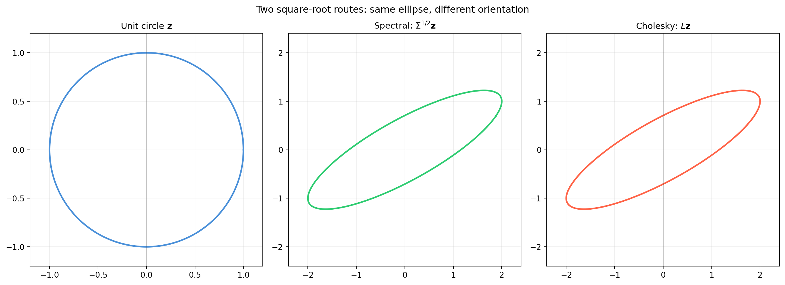
L_true = np.linalg.cholesky(Sigma_true)
n_good = 400
X_good = rng.standard_normal((n_good, 3)) @ L_true.T + mu_good

mu_shriv = np.array([580.0, 0.52, 51.0])
X_shriv  = rng.standard_normal((40, 3)) @ np.linalg.cholesky(
               np.diag([900.0, 0.008, 25.0])).T + mu_shriv

mu_mold = np.array([830.0, 0.70, 35.0])
X_mold  = rng.standard_normal((40, 3)) @ np.linalg.cholesky(
               np.diag([1200.0, 0.005, 20.0])).T + mu_mold

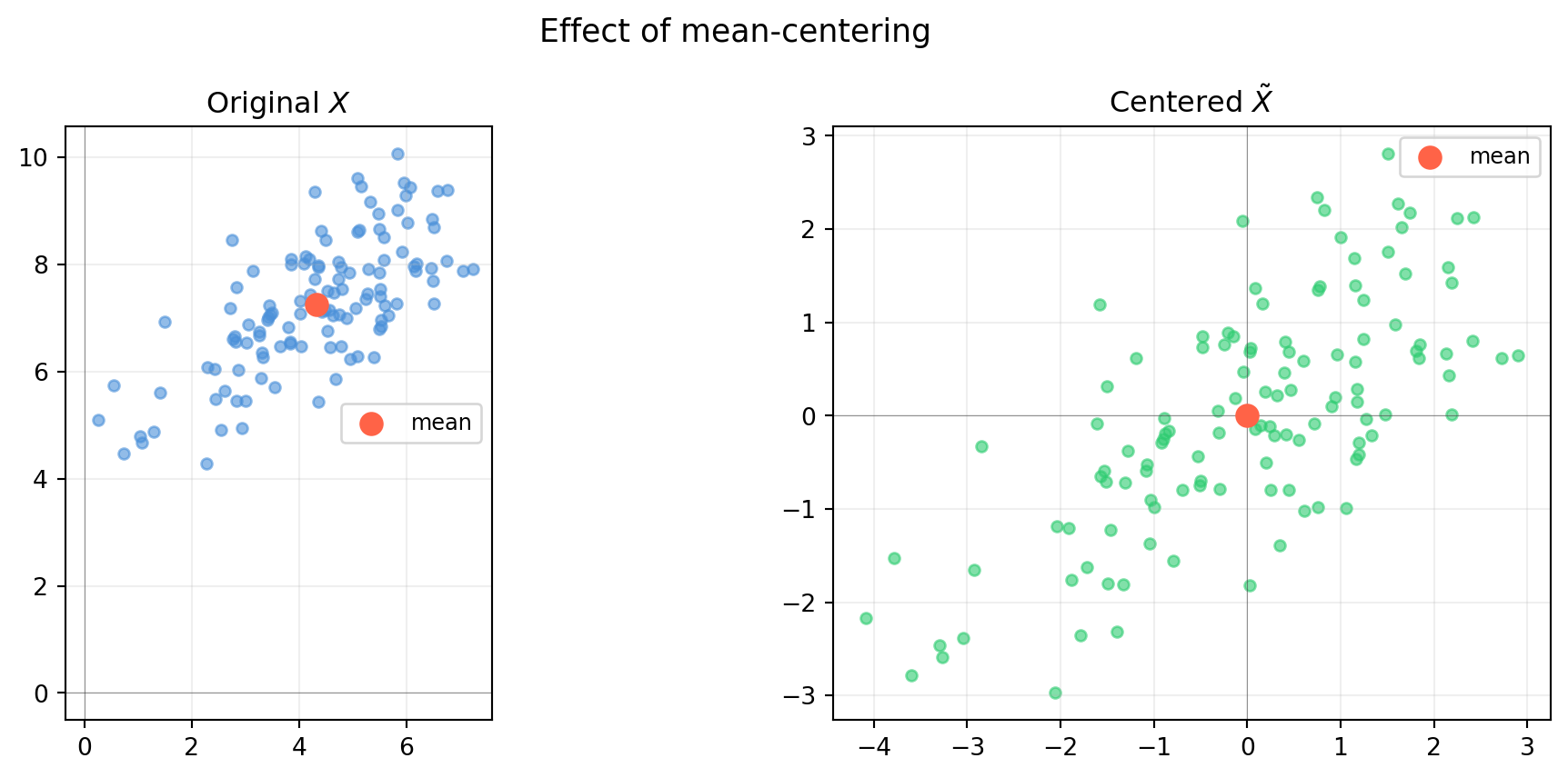
mu_hat    = X_good.mean(axis=0)
X_c       = X_good - mu_hat
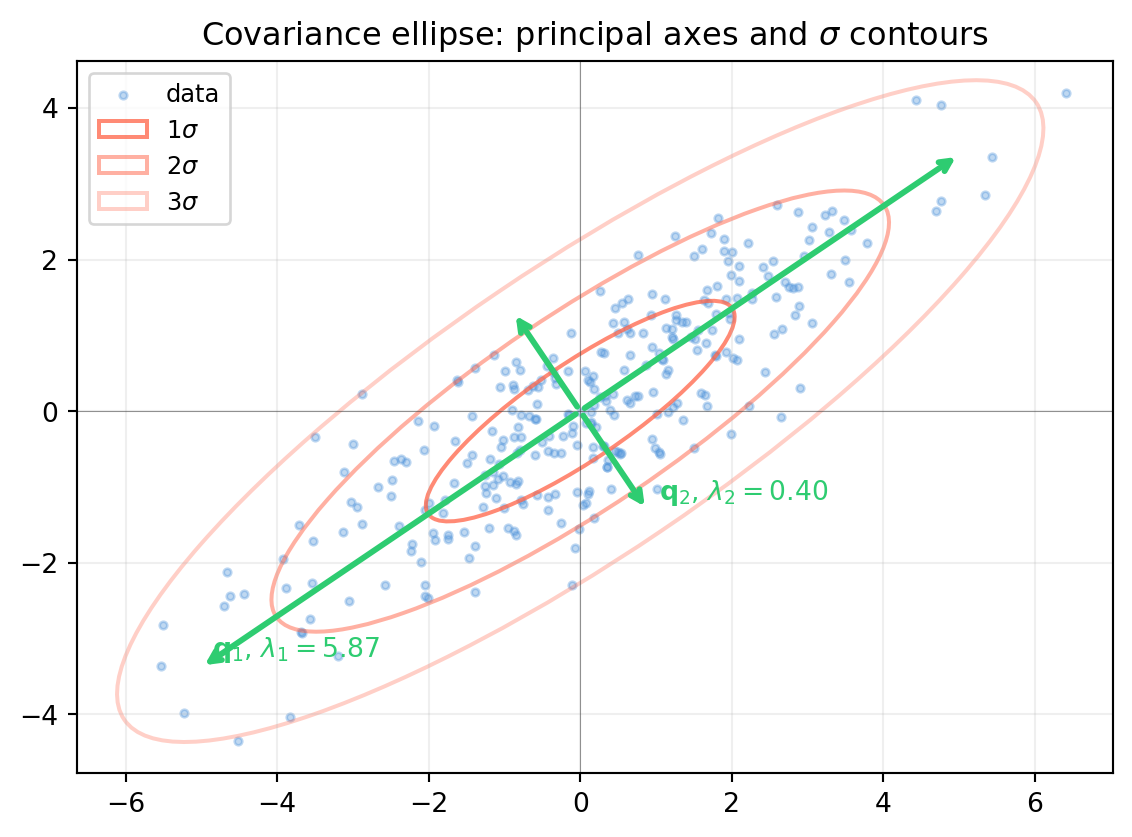
Sigma_hat = X_c.T @ X_c / (n_good - 1)
L_hat     = np.linalg.cholesky(Sigma_hat)

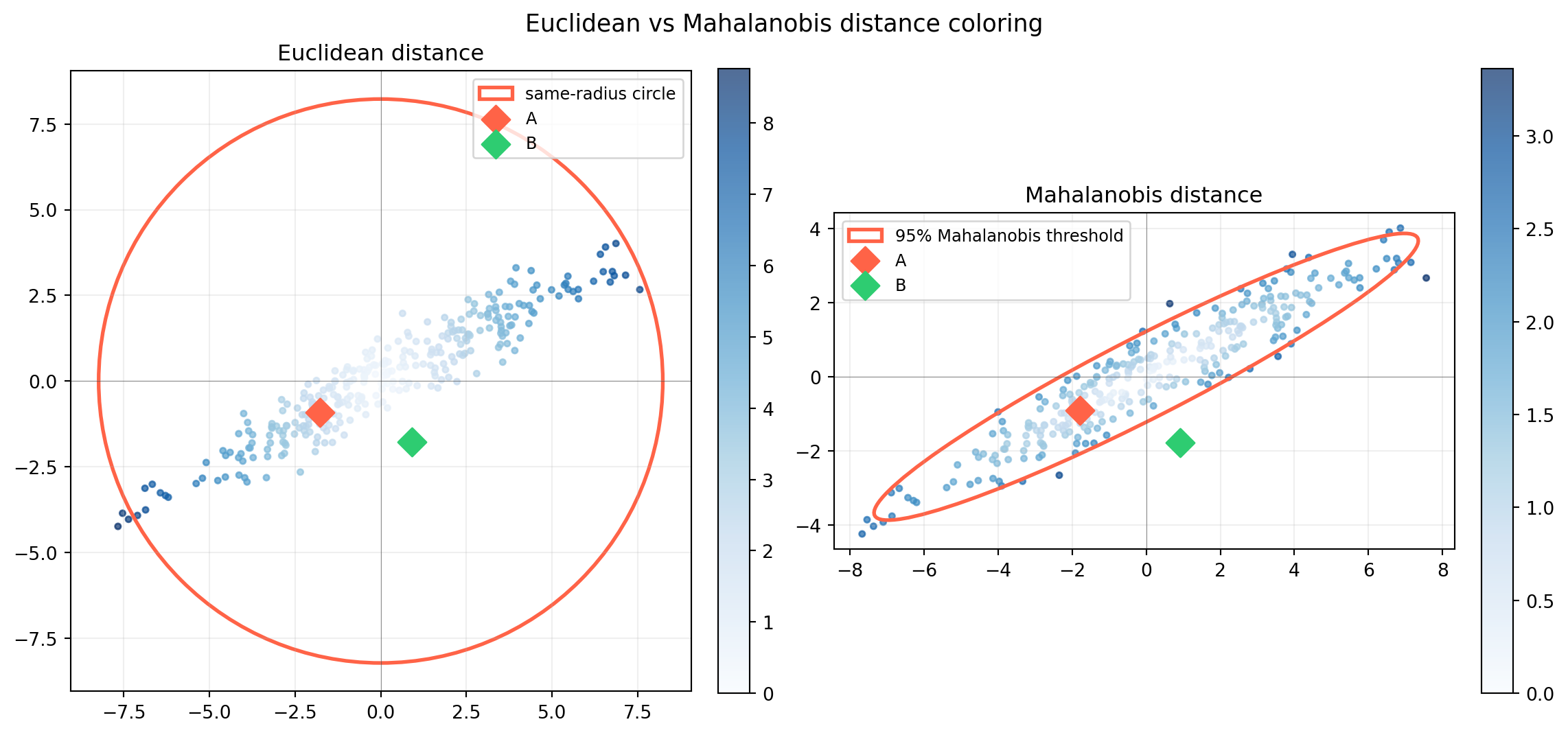
def mahalanobis(X, mu, L):
    diff = X - mu
    Z    = np.linalg.solve(L, diff.T).T
    return np.linalg.norm(Z, axis=1)

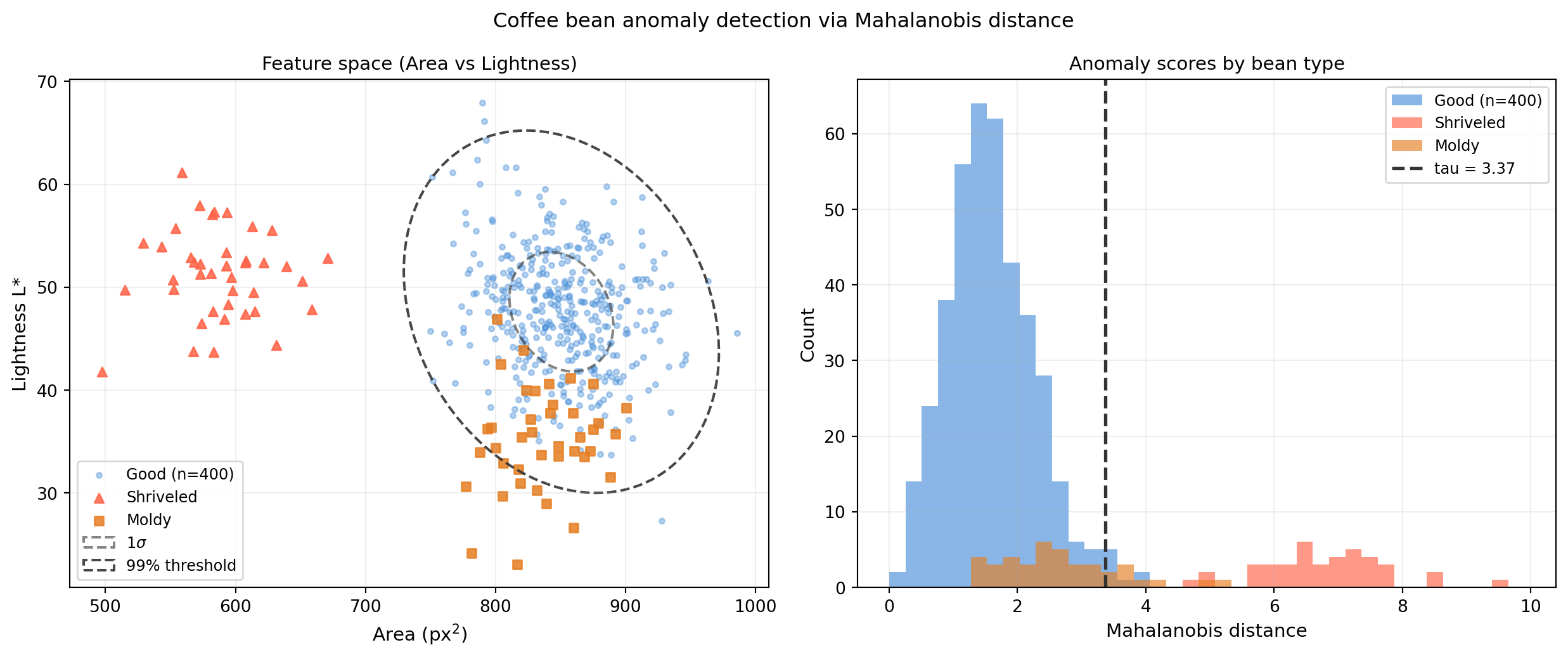
tau = np.sqrt(chi2.ppf(0.99, df=3))
d_good  = mahalanobis(X_good,  mu_hat, L_hat)
d_shriv = mahalanobis(X_shriv, mu_hat, L_hat)
d_mold  = mahalanobis(X_mold,  mu_hat, L_hat)

# Project to 2-D subspace: Area (feat 0) vs Lightness (feat 2) for visualization
feat_x, feat_y = 0, 2
labels_x = ['Area (px$^2$)', 'Eccentricity', 'Lightness L*']

# Marginal covariance for the 2-D projection
idx2 = [feat_x, feat_y]
Sigma_2d = Sigma_hat[np.ix_(idx2, idx2)]     # shape (2, 2)
mu_2d    = mu_hat[idx2]                       # shape (2,)
lam2, Q2 = np.linalg.eigh(Sigma_2d)
ord2 = np.argsort(lam2)[::-1]
lam2 = lam2[ord2];  Q2 = Q2[:, ord2]
angle2 = np.degrees(np.arctan2(Q2[1, 0], Q2[0, 0]))

fig, axes = plt.subplots(1, 2, figsize=(13, 5.5))

# Left: scatter in 2-D feature space
ax = axes[0]
ax.scatter(X_good[:, feat_x],  X_good[:, feat_y],
           s=10, color='#4a90d9', alpha=0.4, label=f'Good (n={n_good})')
ax.scatter(X_shriv[:, feat_x], X_shriv[:, feat_y],
           s=30, color='tomato', alpha=0.85, marker='^', label='Shriveled')
ax.scatter(X_mold[:, feat_x],  X_mold[:, feat_y],
           s=30, color='#e67e22', alpha=0.85, marker='s', label='Moldy')

# 99% Mahalanobis ellipse (marginal 2-D; chi2 df=2 for 2-D projection)
tau_2d = np.sqrt(chi2.ppf(0.99, df=2))
for n_sig, alpha_ell in [(1, 0.6), (tau_2d, 0.9)]:
    lbl = '99% threshold' if n_sig == tau_2d else '1$\\sigma$'
    ell = Ellipse(xy=mu_2d,
                  width  = 2 * n_sig * np.sqrt(lam2[0]),
                  height = 2 * n_sig * np.sqrt(lam2[1]),
                  angle=angle2, edgecolor='#333333', facecolor='none',
                  lw=1.5, linestyle='--', alpha=alpha_ell, label=lbl)
    ax.add_patch(ell)
ax.set_xlabel(labels_x[feat_x], fontsize=11)
ax.set_ylabel(labels_x[feat_y], fontsize=11)
ax.set_title('Feature space (Area vs Lightness)', fontsize=11)
ax.legend(fontsize=9)
ax.grid(alpha=0.2)

# Right: Mahalanobis distance histogram
ax2 = axes[1]
all_d = np.concatenate([d_good, d_shriv, d_mold])
bins  = np.linspace(0, all_d.max() * 1.05, 40)
ax2.hist(d_good,  bins=bins, color='#4a90d9', alpha=0.65, label=f'Good (n={n_good})')
ax2.hist(d_shriv, bins=bins, color='tomato',  alpha=0.65, label='Shriveled')
ax2.hist(d_mold,  bins=bins, color='#e67e22', alpha=0.65, label='Moldy')
ax2.axvline(tau, color='#333333', lw=2, linestyle='--', label=f'tau = {tau:.2f}')
ax2.set_xlabel('Mahalanobis distance', fontsize=11)
ax2.set_ylabel('Count', fontsize=11)
ax2.set_title('Anomaly scores by bean type', fontsize=11)
ax2.legend(fontsize=9)
ax2.grid(alpha=0.2)

fig.suptitle('Coffee bean anomaly detection via Mahalanobis distance', fontsize=12)
fig.tight_layout()
plt.savefig('ch19-covariance/fig-coffee-anomaly.png', dpi=150, bbox_inches='tight')
plt.show()

19.8.4 Key Takeaways

One-class classification requires only inlier data. No labeled defective examples are needed during training – only an estimate of \(\boldsymbol{\mu}\) and \(\Sigma\) from good beans. The chi-squared threshold provides a theoretically grounded false positive rate.
Mahalanobis handles correlated features without hand-tuning. If area and eccentricity are correlated (larger beans tend to be more circular), a point deviating in both features simultaneously might be only mildly surprising. Mahalanobis accounts for this; a per-feature threshold would not.
Detection power depends on defect type. Shriveled beans (small, eccentric) are easily detected because they deviate far in the Area dimension. Moldy beans (same shape, lighter color) are detected via the Lightness feature. A single Euclidean threshold would miss moldy beans entirely.
Regularize in production. With \(p = 3\) and \(n = 400\), the sample covariance is well-conditioned. In practice with \(p\) large (color histograms, texture features), add a ridge term \(\Sigma \leftarrow \Sigma + \epsilon I\) or use a shrinkage estimator (Ledoit-Wolf) before inverting.

19.9 Solutions

19.9.1 Mean-Centering and the Data Matrix

19.1.1 \(H^2 = (I - \frac{1}{n}\mathbf{1}\mathbf{1}^T)^2 = I - \frac{2}{n}\mathbf{1}\mathbf{1}^T + \frac{1}{n^2}\mathbf{1}\mathbf{1}^T\mathbf{1}\mathbf{1}^T = I - \frac{2}{n}\mathbf{1}\mathbf{1}^T + \frac{n}{n^2}\mathbf{1}\mathbf{1}^T = I - \frac{1}{n}\mathbf{1}\mathbf{1}^T = H\). \(H\mathbf{1} = \mathbf{1} - \frac{1}{n}\mathbf{1}\mathbf{1}^T\mathbf{1} = \mathbf{1} - \mathbf{1} = \mathbf{0}\). Idempotency means applying \(H\) twice gives the same result as once: \(H\) is an orthogonal projection onto the subspace orthogonal to \(\mathbf{1}\), and projecting onto a subspace is a “one-shot” operation.

19.1.2 Let \(X' = X + \mathbf{1}\mathbf{c}^T\). Mean: \(\bar{\mathbf{x}}' = \bar{\mathbf{x}} + \mathbf{c}\). Centered: \(X' - \mathbf{1}\bar{\mathbf{x}}'^T = X + \mathbf{1}\mathbf{c}^T - \mathbf{1}(\bar{\mathbf{x}} + \mathbf{c})^T = X - \mathbf{1}\bar{\mathbf{x}}^T = \tilde{X}\). Equivalently, \(HX' = HX + H\mathbf{1}\mathbf{c}^T = HX\) since \(H\mathbf{1} = \mathbf{0}\).

19.1.3 Column-centering ensures \(\tilde{X}^T\mathbf{1}_n = \mathbf{0}\) (each column sums to zero), but says nothing about row sums. The row sum \(\tilde{X}\mathbf{1}_p\) is \(\sum_j \tilde{X}_{ij}\) for each row \(i\), which is generally non-zero. Double-centering (\(H_n X H_p\) with both the row and column centering matrices) forces both row and column sums to zero. This is used in collaborative filtering (e.g., Netflix matrix) to remove user and item biases simultaneously.

19.1.4 When \(\bar{\mathbf{x}} = \mathbf{0}\) exactly, \(\tilde{X} = X\) so \(\frac{1}{n-1}X^TX = \frac{n}{n-1} \cdot \frac{1}{n}X^TX\). As \(n \to \infty\), \(n/(n-1) \to 1\), so the two converge. For finite \(n\), dividing by \(n-1\) rather than \(n\) gives an unbiased estimator of the population covariance: \(\mathbb{E}[\frac{1}{n-1}\tilde{X}^T\tilde{X}] = \Sigma_{\text{pop}}\) (Bessel’s correction). Dividing by \(n\) gives the maximum-likelihood estimator, which is biased downward.

19.9.2 The Covariance Matrix

19.2.1 The \((j,k)\) entry of \(\tilde{X}^T\tilde{X}\) is \((\tilde{X}^T\tilde{X})_{jk} = \sum_{i=1}^n (\tilde{X}^T)_{ji}\tilde{X}_{ik} = \sum_{i=1}^n \tilde{X}_{ij}\tilde{X}_{ik}\). Dividing by \(n-1\) gives \(\Sigma_{jk}\).

19.2.2 \(\mathbf{v}^T\Sigma\mathbf{v} = \frac{1}{n-1}\mathbf{v}^T\tilde{X}^T\tilde{X}\mathbf{v} = \frac{1}{n-1}\|\tilde{X}\mathbf{v}\|_2^2 \ge 0\). Equality holds iff \(\tilde{X}\mathbf{v} = \mathbf{0}\), i.e., \(\mathbf{v} \in \text{Null}(\tilde{X})\). This happens when \(\mathbf{v}\) is a linear combination of features that is identically zero across all observations (e.g., a feature that is a constant multiple of another).

19.2.3 \(\Sigma_{jk} = 0\) means features \(j\) and \(k\) are orthogonal in the centered data. Geometrically, the covariance ellipse has no tilt between those two feature axes – the projection onto the \((j,k)\) plane is an axis-aligned ellipse. Two features can be uncorrelated (\(\Sigma_{jk} = 0\)) yet dependent: for example, if \(x_j \sim \text{Uniform}(-1,1)\) and \(x_k = x_j^2\), then \(\text{Cov}(x_j, x_k) = 0\) but knowing \(x_j\) determines \(x_k\).

19.2.4 \(R_{jk} = \Sigma_{jk}/\sqrt{\Sigma_{jj}\Sigma_{kk}} = (D^{-1/2})_{jj}\Sigma_{jk}(D^{-1/2})_{kk}\) \(= (D^{-1/2}\Sigma D^{-1/2})_{jk}\). Diagonal entries: \(R_{jj} = \Sigma_{jj}/\sqrt{\Sigma_{jj}}\sqrt{\Sigma_{jj}} = \Sigma_{jj}/\Sigma_{jj} = 1\). Each feature is perfectly correlated with itself.

19.9.3 The Multivariate Gaussian and Its Geometry

19.3.1 For \(\mathbf{z} \sim \mathcal{N}(\mathbf{0}, I_2)\), \(\|\mathbf{z}\|^2 \sim \chi^2_2\). The \(\chi^2_2\) CDF is \(F(k^2) = 1 - e^{-k^2/2}\). At \(k = 1\): \(P(\|\mathbf{z}\|^2 \le 1) = 1 - e^{-1/2} \approx 0.393\). So the 2-D 1-sigma ellipsoid contains only \(39.3\%\) of the mass, not \(68\%\). The curse of dimensionality: as \(p\) increases, the 1-sigma ellipsoid captures an ever smaller fraction of mass.

19.3.2 The moment generating function of \(A\mathbf{x}\) at \(\mathbf{t}\) is \(\mathbb{E}[e^{\mathbf{t}^T A\mathbf{x}}] = e^{\mathbf{t}^T A\boldsymbol{\mu} + \frac{1}{2}\mathbf{t}^T A\Sigma A^T \mathbf{t}}\), which is the MGF of \(\mathcal{N}(A\boldsymbol{\mu}, A\Sigma A^T)\). When \(m < p\), \(A\Sigma A^T \in \mathbb{R}^{m \times m}\) has rank at most \(m\); the image is an \(m\)-dimensional Gaussian. The original density (in \(\mathbb{R}^p\)) is degenerate (concentrated on the \(m\)-dim subspace \(\text{Col}(A^T)\)) and has no density with respect to Lebesgue measure in \(\mathbb{R}^p\).

19.3.3 The block \(\Sigma\) is PSD, so for any \(\mathbf{v}\), \(\mathbf{v}^T\Sigma\mathbf{v} \ge 0\). Take \(\mathbf{v} = [\mathbf{v}_A^T, -\Sigma_{BB}^{-1}\Sigma_{BA}\mathbf{v}_A^T]^T\): \(\mathbf{v}^T\Sigma\mathbf{v} = \mathbf{v}_A^T(\Sigma_{AA} - \Sigma_{AB}\Sigma_{BB}^{-1}\Sigma_{BA})\mathbf{v}_A \ge 0\). So the Schur complement is PSD. Since \(\Sigma_{AA} - (\Sigma_{AA} - \Sigma_{AB}\Sigma_{BB}^{-1}\Sigma_{BA}) = \Sigma_{AB}\Sigma_{BB}^{-1}\Sigma_{BA}\) is PSD (as \(\Sigma_{BB}^{-1}\) is PSD), we have \(\Sigma_{AA} \succeq \Sigma_{AA} - \Sigma_{AB}\Sigma_{BB}^{-1}\Sigma_{BA}\).

19.3.4 The change-of-variables from \(\mathbf{x}\) to \(\mathbf{z} = \Sigma^{-1/2}(\mathbf{x} - \boldsymbol{\mu})\) has Jacobian \(|\partial\mathbf{x}/\partial\mathbf{z}| = |\Sigma^{1/2}| = |\Sigma|^{1/2}\) (the determinant of the linear map). To keep \(\int p\, d\mathbf{x} = 1\) after the change of variables, the normalizer picks up a factor of \(|\Sigma|^{1/2}\) from the volume scaling.

19.9.4 Mahalanobis Distance

19.4.1 \(d_M(\mathbf{x})^2 = (\mathbf{x}-\boldsymbol{\mu})^T (\sigma^2 I)^{-1} (\mathbf{x}-\boldsymbol{\mu}) = \|\mathbf{x}-\boldsymbol{\mu}\|^2/\sigma^2\). So \(d_M = \|\mathbf{x}-\boldsymbol{\mu}\|/\sigma\). Euclidean distance is Mahalanobis distance with \(\Sigma = I\) (isotropic unit variance); it treats all directions and scales equally.

19.4.2 \(\Sigma = \text{diag}(1, 100)\), \(\mathbf{x} = (0, 5)^T\), \(\boldsymbol{\mu} = \mathbf{0}\). Euclidean: \(\|(0,5)\| = 5\). Mahalanobis: \(\sqrt{0^2/1 + 5^2/100} = \sqrt{0.25} = 0.5\). The Mahalanobis distance of \(0.5\) correctly reflects that a deviation of 5 units in a feature with standard deviation 10 is only half a standard deviation – not surprising. Euclidean would flag this as anomalous.

19.4.3 With centered \(X\), the leverage score \(h_{ii} = \mathbf{x}_i^T(X^TX)^{-1}\mathbf{x}_i\). The sample covariance is \(\Sigma = X^TX/(n-1)\), so \((X^TX)^{-1} = \Sigma^{-1}/(n-1)\). Thus \(h_{ii} = \mathbf{x}_i^T\Sigma^{-1}\mathbf{x}_i/(n-1) = d_M^2(\mathbf{x}_i)/(n-1)\) (with \(\boldsymbol{\mu} = \mathbf{0}\) since \(X\) is centered). High-leverage points are Mahalanobis-far from the centroid.

19.4.4 \(\mathbf{z} = \Sigma^{-1/2}(\mathbf{x}-\boldsymbol{\mu})\). Since \(\mathbf{x} \sim \mathcal{N}(\boldsymbol{\mu},\Sigma)\), we have \(\mathbf{z} = \Sigma^{-1/2}(\mathbf{x}-\boldsymbol{\mu}) \sim \mathcal{N}(\mathbf{0}, \Sigma^{-1/2}\Sigma\Sigma^{-1/2}) = \mathcal{N}(\mathbf{0}, I_p)\). Then \(d_M^2 = \|\mathbf{z}\|^2 = \sum_{j=1}^p z_j^2\), a sum of \(p\) independent standard normal squares, which is \(\chi^2_p\) by definition.

19.9.5 The Matrix Square Root \(\Sigma^{1/2}\)

19.5.1 \(\Sigma = \begin{bmatrix}2&1\\1&2\end{bmatrix}\). Eigenvalues: \(\det(\Sigma - \lambda I) = (2-\lambda)^2 - 1 = 0 \Rightarrow \lambda = 1, 3\). Eigenvectors: \(\lambda_1 = 3\), \(\mathbf{q}_1 = \frac{1}{\sqrt{2}}(1,1)^T\); \(\lambda_2 = 1\), \(\mathbf{q}_2 = \frac{1}{\sqrt{2}}(-1,1)^T\). \(\Sigma^{1/2} = \sqrt{3}\,\mathbf{q}_1\mathbf{q}_1^T + 1\,\mathbf{q}_2\mathbf{q}_2^T = \frac{1}{2}\begin{bmatrix}\sqrt{3}+1 & \sqrt{3}-1\\\sqrt{3}-1 & \sqrt{3}+1\end{bmatrix}\). Verification: \((\Sigma^{1/2})^2 = Q\text{diag}(3,1)Q^T = \Sigma\).

19.5.2 Example: \(\Sigma = \begin{bmatrix}4&2\\2&2\end{bmatrix}\). Cholesky: \(L = \begin{bmatrix}2&0\\1&1\end{bmatrix}\) (\(L\) is lower triangular, not symmetric). Spectral: \(\Sigma^{1/2}\) is symmetric (as computed from eigenvectors). Since \(L\) is not symmetric, \(L \ne \Sigma^{1/2}\). Both satisfy \((\cdot)(\cdot)^T = \Sigma\).

19.5.3 For \(\Sigma = Q\Lambda Q^T\): \(e^\Sigma = \sum_{k=0}^\infty \Sigma^k / k! = Q\left(\sum_{k=0}^\infty \Lambda^k/k!\right)Q^T = Q\,e^\Lambda\,Q^T\), where \(e^\Lambda = \text{diag}(e^{\lambda_1}, \ldots, e^{\lambda_p})\). Functions of normal matrices are computed by applying the scalar function to the eigenvalues.

19.5.4 Factorization cost: both spectral and Cholesky are \(O(p^3)\). Per-draw cost (once \(A\) is known): computing \(A\mathbf{z}\) for one draw costs \(O(p^2)\), so \(n\) draws cost \(O(np^2)\). The factorization dominates when \(O(p^3) \gg O(np^2)\), i.e., \(p \gg n\). For \(p = 100\): factorization \(\sim 10^6\) flops; draw cost \(\sim n \cdot 10^4\) flops. Factorization dominates until \(n \approx 100\); for \(n \gg 100\) (certainly for \(n = 10^5\)), the draw cost \(O(np^2) = O(10^9)\) dominates. The factorization is a one-time \(O(p^3)\) investment.

19.9.6 Whitening: ZCA and PCA

19.6.1 \(W_{\text{ZCA}}\Sigma W_{\text{ZCA}}^T = \Sigma^{-1/2}\Sigma\Sigma^{-1/2} = I\) since \(\Sigma^{-1/2}\) is symmetric. For minimality: write \(W = R\Sigma^{-1/2}\) for some orthogonal \(R\) (all solutions are of this form). Then \(\|W - I\|_F^2 = \|R\Sigma^{-1/2} - I\|_F^2\). Using \(\|AB\|_F \ge \|\sigma_{\min}(A)\| \cdot \|B\|_F\) and the unitary invariance of the Frobenius norm, the minimum over orthogonal \(R\) is achieved at \(R = I\) (Procrustes argument), giving \(W = \Sigma^{-1/2}\).

19.6.2 \(W_k = \Lambda_k^{-1/2} Q_k^T\) where \(Q_k\) holds the top \(k\) eigenvectors and \(\Lambda_k = \text{diag}(\lambda_1,\ldots,\lambda_k)\). \(W_k\Sigma W_k^T = \Lambda_k^{-1/2}Q_k^T(Q\Lambda Q^T)Q_k\Lambda_k^{-1/2} = \Lambda_k^{-1/2}\Lambda_k\Lambda_k^{-1/2} = I_k\). This simultaneously projects to the top-\(k\) PC space and whitens – one matrix-vector multiply instead of two separate operations.

19.6.3 \(\Sigma^{-1/2} = Q\Lambda^{-1/2}Q^T\) with \(\Lambda^{-1/2} = \text{diag}(1/\sqrt{\lambda_j})\). When \(\lambda_j \approx 0\), \(1/\sqrt{\lambda_j} \to \infty\) – the whitening transform amplifies negligible variation to unit scale, magnifying numerical noise. Regularized: \(W_\epsilon = Q(\Lambda + \epsilon I)^{-1/2}Q^T\), which caps the amplification at \(1/\sqrt{\epsilon}\) in the near-zero directions.

19.6.4 Let \(\Sigma = \begin{bmatrix}1 & 0.99 \\ 0.99 & 1\end{bmatrix}\). \(D = I\), so \(D^{-1/2}\Sigma D^{-1/2} = \Sigma\). After batch normalization, the residual covariance is still \(\Sigma\) – off-diagonal entry \(0.99\) is unchanged. Scalar batch normalization does nothing when variances are already equal; the correlation structure remains fully intact.

19.9.7 Information Form: \(\Omega = \Sigma^{-1}\)

19.7.1 The conditional of \((x_j, x_k)\) given the rest has covariance \((\Omega_{\{j,k\},\{j,k\}})^{-1}\) (the inverse of the \(2\times 2\) block of \(\Omega\) indexed by \(\{j,k\}\)). When \(\Omega_{jk} = 0\), this block is diagonal: \(\Omega_{\{j,k\},\{j,k\}} = \text{diag}(\Omega_{jj}, \Omega_{kk})\), so the conditional covariance is also diagonal, meaning \(x_j\) and \(x_k\) are conditionally independent.

19.7.2 The likelihood of \(\mathbf{x}\) given \(\mathbf{y}_1, \mathbf{y}_2\) factors as \(p(\mathbf{y}_1|\mathbf{x})p(\mathbf{y}_2|\mathbf{x})\). Each factor contributes \(-\frac{1}{2}(y_i - H_i\mathbf{x})^TR_i^{-1}(y_i - H_i\mathbf{x})\) to the log-likelihood, which expands to \(-\frac{1}{2}\mathbf{x}^T H_i^TR_i^{-1}H_i\mathbf{x} + \mathbf{x}^T H_i^TR_i^{-1}\mathbf{y}_i + \text{const}\). Summing: \(\Omega_{\text{post}} = H_1^TR_1^{-1}H_1 + H_2^TR_2^{-1}H_2\), \(\boldsymbol{\eta}_{\text{post}} = H_1^TR_1^{-1}\mathbf{y}_1 + H_2^TR_2^{-1}\mathbf{y}_2\).

19.7.3 A \(p \times p\) tridiagonal system has bandwidth \(b = 1\). Banded Cholesky (forward elimination) requires \(O(pb^2) = O(p)\) operations – linear in the number of poses. The dense case requires \(O(p^3)\). For \(T = 1000\) poses, the tridiagonal system solves in \(\sim 10^3\) flops vs. \(\sim 10^9\) for the dense matrix – a factor of \(10^6\) speedup.

19.7.4 Suppose poses \(i\) and \(k\) (\(i < k\)) both observed landmark \(l\). After marginalizing out \(l\) from the factor \((x_i, l)\) and \((x_k, l)\), the Schur complement introduces a non-zero entry \(\Omega_{ik}\) in the pose-only information matrix: observing the same landmark creates a virtual constraint between two poses, even if they were not directly connected by odometry. Geometrically, “the relative pose between \(i\) and \(k\) is constrained because we both saw landmark \(l\) from different viewpoints.” This is the phenomenon of loop closure in SLAM.