23  State Estimation and Covariance Propagation

23.1 Linear State Estimation

Many physical systems have a hidden state \(\mathbf{x}_k \in \mathbb{R}^n\) that evolves over time according to known dynamics, perturbed by unmodeled forces, thermal noise, or numerical truncation. A sensor observes the state indirectly through measurements that carry their own noise. The goal of state estimation is to form the best possible guess of the hidden state from accumulated observations.

The discrete-time linear state-space model captures this setting in two equations:

\[ \mathbf{x}_{k+1} = A\mathbf{x}_k + B\mathbf{u}_k + \mathbf{w}_k, \qquad \mathbf{w}_k \sim \mathcal{N}(\mathbf{0},\, Q), \tag{23.1} \]

\[ \mathbf{y}_k = H\mathbf{x}_k + \mathbf{v}_k, \qquad \mathbf{v}_k \sim \mathcal{N}(\mathbf{0},\, R). \tag{23.2} \]

Symbol	Dimension	Role
\(A\)	\(n \times n\)	Transition matrix (system dynamics)
\(B\)	\(n \times p\)	Control input matrix
\(\mathbf{u}_k\)	\(p \times 1\)	Known input (motor command, IMU reading)
\(Q\)	\(n \times n\), PSD	Process noise covariance
\(H\)	\(m \times n\)	Observation matrix
\(R\)	\(m \times m\), PD	Measurement noise covariance

The noise vectors \(\mathbf{w}_k\) and \(\mathbf{v}_k\) are mutually independent, uncorrelated across time steps, and independent of the initial state \(\mathbf{x}_0\).

---

23.1.1 Why the Gaussian Assumption?

Gaussian noise is not merely a convenient assumption — it is structurally special. Under jointly Gaussian noise, the posterior distribution \(p(\mathbf{x}_k \mid \mathbf{y}_{1:k})\) is also Gaussian, so it is fully described by its mean and covariance. No other distribution family has this closure property under linear transformations.

This means the optimal estimator — the one minimizing the mean squared error \(\mathbb{E}[\|\mathbf{x}_k - \hat{\mathbf{x}}_k\|^2]\) over all estimators, linear or nonlinear — has the form

\[ \hat{\mathbf{x}}_k = G_1\mathbf{y}_1 + G_2\mathbf{y}_2 + \cdots + G_k\mathbf{y}_k + \mathbf{g}_0, \]

and the Kalman filter computes the optimal gain matrices \(G_i\) recursively without ever storing the full measurement history.

When the noise is non-Gaussian, the Kalman filter remains the best linear unbiased estimator (BLUE): the linear function of the measurements with the smallest possible covariance. It may no longer be globally optimal, but it is the best achievable by any linear filter.

---

23.1.2 The Kalman Filter: Two Steps

The Kalman filter propagates a Gaussian belief \(\mathcal{N}(\hat{\mathbf{x}}_{k|k},\, P_{k|k})\) forward in time via two alternating steps.

Predict (propagate belief through dynamics):

\[ \hat{\mathbf{x}}_{k+1|k} = A\hat{\mathbf{x}}_{k|k} + B\mathbf{u}_k, \tag{23.3} \] \[ P_{k+1|k} = AP_{k|k}A^T + Q. \tag{23.4} \]

The subscript \(k+1|k\) means “estimate of \(\mathbf{x}_{k+1}\) given measurements up to time \(k\)”. The prediction is unbiased because \(\mathbb{E}[\mathbf{w}_k] = \mathbf{0}\). The covariance grows: \(AP_{k|k}A^T\) deforms the current uncertainty through the dynamics, and \(Q\) adds fresh process noise.

Update (incorporate new measurement \(\mathbf{y}_{k+1}\)):

\[ K_{k+1} = P_{k+1|k}H^T\!\left(HP_{k+1|k}H^T + R\right)^{-1}, \tag{23.5} \] \[ \hat{\mathbf{x}}_{k+1|k+1} = \hat{\mathbf{x}}_{k+1|k} + K_{k+1}\!\underbrace{\left(\mathbf{y}_{k+1} - H\hat{\mathbf{x}}_{k+1|k}\right)}_{\text{innovation}}, \tag{23.6} \] \[ P_{k+1|k+1} = (I - K_{k+1}H)P_{k+1|k}. \tag{23.7} \]

The innovation \(\boldsymbol{\nu}_{k+1} = \mathbf{y}_{k+1} - H\hat{\mathbf{x}}_{k+1|k}\) measures the discrepancy between the actual and predicted measurement. The Kalman gain \(K_{k+1}\) determines how heavily to weight this discrepancy. Equations (23.4) and (23.5) are derived in §23.2 and §23.3 respectively.

---

23.1.3 Scalar Intuition: Tracking a Slow Drift

Before the full multivariate derivations, the scalar case \(n = m = 1\) already reveals the essential logic. Suppose a sensor platform drifts along a corridor: \(x_{k+1} = x_k + w_k\), \(w_k \sim \mathcal{N}(0, \sigma_w^2)\), observed by a range finder: \(y_k = x_k + v_k\), \(v_k \sim \mathcal{N}(0, \sigma_v^2)\). Here \(A = H = 1\), \(B = 0\).

The scalar Kalman gain reduces to:

\[ k = \frac{P}{P + R}, \]

which lives in \((0, 1)\) and has an immediate interpretation:

• \(P \gg R\): we are far more uncertain about the state than the measurement. Then \(k \approx 1\) — nearly discard the prediction and adopt the measurement.
• \(P \ll R\): the measurement is very noisy relative to our state uncertainty. Then \(k \approx 0\) — stay close to the prediction and downweight the measurement.

The posterior covariance after the update is \(p_{\text{post}} = (1 - k)\,P = PR/(P+R)\), which is strictly smaller than both \(P\) and \(R\). A measurement always reduces uncertainty, even a very noisy one.

---

import numpy as np
import matplotlib.pyplot as plt

rng = np.random.default_rng(231)

A = 1.0      # random walk
Q = 0.5      # process noise variance
H = 1.0      # direct measurement
R = 4.0      # measurement noise variance
n_steps = 60

# Simulate true state and measurements
x_true = np.zeros(n_steps + 1)      # shape (61,)
y_meas = np.zeros(n_steps)          # shape (60,)
for k in range(n_steps):
    x_true[k + 1] = A * x_true[k] + rng.normal(0, np.sqrt(Q))
    y_meas[k] = H * x_true[k + 1] + rng.normal(0, np.sqrt(R))

# Kalman filter
x_hat = np.zeros(n_steps + 1)       # shape (61,)
P_arr = np.zeros(n_steps + 1)       # shape (61,)
P_arr[0] = 10.0                     # large initial uncertainty

for k in range(n_steps):
    # Predict
    x_pred = A * x_hat[k]
    P_pred = A * P_arr[k] * A + Q   # P_{k+1|k}

    # Update
    S     = H * P_pred * H + R      # innovation covariance
    gain  = P_pred * H / S          # Kalman gain
    x_hat[k + 1] = x_pred + gain * (y_meas[k] - H * x_pred)
    P_arr[k + 1] = (1.0 - gain * H) * P_pred

sigma = np.sqrt(P_arr)              # shape (61,)

# Theoretical steady-state: solve p = p + Q - p^2/(p+R) => p^2 - QR/(Q+R)*p...
# scalar Riccati: P_ss = Q/2 + sqrt((Q/2)^2 + QR)  [with A=1]
P_ss = Q / 2.0 + np.sqrt((Q / 2.0) ** 2 + Q * R)

fig, axes = plt.subplots(2, 1, figsize=(10, 6), sharex=True)
t = np.arange(n_steps + 1)

ax = axes[0]
ax.plot(t, x_true, color='#333333', lw=1.5, label='True position', zorder=2)
ax.scatter(np.arange(1, n_steps + 1), y_meas, s=18,
           color='tomato', alpha=0.7, label='Measurements', zorder=3)
ax.plot(t, x_hat, color='#4a90d9', lw=2, label='KF estimate', zorder=4)
ax.fill_between(t, x_hat - 2 * sigma, x_hat + 2 * sigma,
                color='#4a90d9', alpha=0.18, label='2-sigma band')
ax.set_ylabel('Position')
ax.legend(fontsize=9)
ax.grid(alpha=0.2)
ax.axhline(0, color='#333333', lw=0.4, alpha=0.5)

ax = axes[1]
ax.plot(t, P_arr, color='#2ecc71', lw=2, label='Posterior variance $P_{k|k}$')
ax.axhline(P_ss, color='gray', ls='--', lw=1.2,
           label=f'Steady-state $P_\\infty = {P_ss:.3f}$')
ax.set_xlabel('Time step $k$')
ax.set_ylabel('$P$ (variance)')
ax.legend(fontsize=9)
ax.grid(alpha=0.2)

plt.tight_layout()
plt.show()

print(f"Steady-state P (Riccati): {P_ss:.4f}")
print(f"P at final step (filter): {P_arr[-1]:.4f}")

Figure 23.1: Scalar Kalman filter tracking a random walk. Top: true position (gray), noisy measurements (red), KF estimate with 2-sigma band (blue). Bottom: posterior variance P converging to its steady-state value.

Steady-state P (Riccati): 1.6861
P at final step (filter): 1.1861

The variance converges to a steady-state value \(P_\infty\) determined by the discrete algebraic Riccati equation (DARE). For the scalar random walk with \(A=1\), the closed form is \(P_\infty = Q/2 + \sqrt{(Q/2)^2 + QR}\). After convergence the Kalman gain is constant and the filter behaves like a fixed exponential smoother.

---

23.1.4 Initialization

The filter requires an initial belief \((\hat{\mathbf{x}}_{0|0},\, P_{0|0})\).

• If the initial state is known exactly: \(P_{0|0} = 0\) (or a small multiple of machine epsilon times \(I\)).
• If the initial state is uncertain: set \(P_{0|0} = \sigma_{\text{init}}^2 I\) with \(\sigma_{\text{init}}\) chosen larger than the expected state magnitude. The filter self-corrects within a few steps regardless of this choice, provided \(P_{0|0}\) is positive definite.

The common mistake of setting \(P_{0|0} = 0\) for an unknown initial state causes the first Kalman gain \(K_1 \approx 0\), so the first measurement does nothing — convergence is delayed or never achieved.

23.2 Covariance Propagation

The predict step of the Kalman filter maps the current belief \(\mathcal{N}(\hat{\mathbf{x}}_{k|k},\, P_{k|k})\) forward through the dynamics \(\mathbf{x}_{k+1} = A\mathbf{x}_k + B\mathbf{u}_k + \mathbf{w}_k\). The mean update \(\hat{\mathbf{x}}_{k+1|k} = A\hat{\mathbf{x}}_{k|k} + B\mathbf{u}_k\) is immediate, but the covariance update requires a short derivation.

---

23.2.1 Derivation

Define the prior prediction error at step \(k+1\):

\[ \mathbf{e}_{k+1|k} = \mathbf{x}_{k+1} - \hat{\mathbf{x}}_{k+1|k}. \]

Substituting the state equation and the predicted mean:

\[ \mathbf{e}_{k+1|k} = \bigl(A\mathbf{x}_k + B\mathbf{u}_k + \mathbf{w}_k\bigr) - \bigl(A\hat{\mathbf{x}}_{k|k} + B\mathbf{u}_k\bigr) = A\underbrace{(\mathbf{x}_k - \hat{\mathbf{x}}_{k|k})}_{\mathbf{e}_{k|k}} + \mathbf{w}_k. \]

The predicted covariance is:

\[ P_{k+1|k} = \mathbb{E}\!\left[\mathbf{e}_{k+1|k}\mathbf{e}_{k+1|k}^T\right] = \mathbb{E}\!\left[(A\mathbf{e}_{k|k} + \mathbf{w}_k)(A\mathbf{e}_{k|k} + \mathbf{w}_k)^T\right]. \]

Expanding and using the independence of \(\mathbf{w}_k\) from \(\mathbf{e}_{k|k}\) (process noise is independent of past state errors) and \(\mathbb{E}[\mathbf{w}_k] = \mathbf{0}\):

\[ P_{k+1|k} = A\,\mathbb{E}\!\left[\mathbf{e}_{k|k}\mathbf{e}_{k|k}^T\right]A^T + \mathbb{E}\!\left[\mathbf{w}_k\mathbf{w}_k^T\right] = \boxed{AP_{k|k}A^T + Q.} \tag{23.4} \]

The cross-terms \(A\,\mathbb{E}[\mathbf{e}_{k|k}\mathbf{w}_k^T] = 0\) because \(\mathbf{w}_k\) is independent of everything before time \(k\).

---

23.2.2 Geometric Meaning

Each term in \(P_{k+1|k} = AP_{k|k}A^T + Q\) has a clear geometric role:

\(AP_{k|k}A^T\): the dynamics deform the uncertainty ellipsoid. If \(P_{k|k} = I\) (spherical uncertainty) and \(A\) has singular values \(\sigma_1 \geq \sigma_2\), then \(AP_{k|k}A^T\) is an ellipse with semi-axes \(\sigma_1\) and \(\sigma_2\). A contracting system (\(\|\sigma_i\| < 1\)) shrinks the ellipsoid; an expanding one grows it.

\(Q\): the process noise inflates the ellipsoid. \(Q\) adds uncertainty in all directions simultaneously. For \(Q = q^2 I\) (isotropic), every axis of the ellipsoid grows by \(q^2\), independent of the dynamics.

Together, the predicted covariance is the Minkowski sum of the dynamically deformed current uncertainty and the process noise uncertainty.

---

23.2.3 Long-Horizon Behavior

Iterating the prediction-only recursion (no updates, \(Q = \text{const}\)):

\[ P_{k+1|k} = A^k P_{0|0} (A^k)^T + \sum_{j=0}^{k-1} A^j Q (A^j)^T. \]

If \(A\) is stable (all eigenvalues satisfy \(|\lambda_i| < 1\)), the first term decays to zero and the sum converges. The steady-state covariance (prediction only, no measurements) satisfies \(P_\infty = AP_\infty A^T + Q\), the discrete Lyapunov equation.

If \(A\) is unstable (\(|\lambda_i| > 1\) for some \(i\)), uncertainty grows without bound in the absence of measurements. This is the mathematical statement that an unstable system is unknowable without sensing.

---

import numpy as np
import matplotlib.pyplot as plt
import matplotlib.patches as mpatches

def draw_ellipse(ax, mean, cov, color, alpha=1.0, fill=False, zorder=2):
    """Draw a 2-sigma covariance ellipse."""
    vals, vecs = np.linalg.eigh(cov)            # shape (2,), (2, 2)
    angle = np.degrees(np.arctan2(vecs[1, 1], vecs[0, 1]))
    width, height = 2 * 2 * np.sqrt(vals[::-1]) # 2-sigma axes
    ellipse = mpatches.Ellipse(
        xy=mean[:2],
        width=width, height=height,
        angle=angle,
        edgecolor=color, facecolor=color if fill else 'none',
        alpha=alpha, lw=1.5, zorder=zorder
    )
    ax.add_patch(ellipse)

rng = np.random.default_rng(232)

# 2D state, no measurements
Q = np.diag([0.05, 0.05])           # shape (2, 2) -- small isotropic process noise
P0 = np.eye(2) * 0.5                # shape (2, 2)
x0 = np.array([0.0, 0.0])          # shape (2,)
n_steps = 15

configs = [
    {'A': np.array([[0.9, 0.2], [0.0, 0.8]]),
     'label': 'Contracting ($|\\lambda|<1$)'},
    {'A': np.array([[1.05, 0.1], [0.0, 1.0]]),
     'label': 'Diverging ($|\\lambda|\\geq 1$)'},
]

colors = ['#4a90d9', '#2ecc71']
fig, axes = plt.subplots(1, 2, figsize=(11, 5))

for ax, cfg, col in zip(axes, configs, colors):
    A = cfg['A']                    # shape (2, 2)
    P = P0.copy()                   # shape (2, 2)
    x = x0.copy()                   # shape (2,)

    eig_vals = np.abs(np.linalg.eigvals(A))

    for step in range(n_steps + 1):
        is_last = (step == n_steps)
        if step % 3 == 0 or is_last:
            alpha_val = 0.3 + 0.7 * (step / n_steps)
            draw_ellipse(ax, x, P, color=col,
                         alpha=alpha_val, fill=is_last, zorder=2 + step)
            ax.plot(*x[:2], 'o', color=col, ms=4, alpha=alpha_val, zorder=10)

        if step < n_steps:
            P = A @ P @ A.T + Q     # shape (2, 2)
            x = A @ x               # shape (2,)

    ax.set_xlim(-4, 4)
    ax.set_ylim(-4, 4)
    ax.set_aspect('equal')
    ax.grid(alpha=0.2)
    ax.axhline(0, color='#333333', lw=0.4, alpha=0.5)
    ax.axvline(0, color='#333333', lw=0.4, alpha=0.5)
    ax.set_xlabel('$x_1$')
    ax.set_ylabel('$x_2$')
    lam_str = ', '.join([f'{v:.2f}' for v in np.linalg.eigvals(A)])
    ax.set_title(f"{cfg['label']}\n$\\lambda(A) = [{lam_str}]$", fontsize=10)

    # Show final P eigenvalues
    final_eigs = np.linalg.eigvals(P)
    print(f"{cfg['label']}: final P eigenvalues = {np.sort(final_eigs)[::-1].round(3)}")

plt.tight_layout()
plt.show()

Contracting ($|\lambda|<1$): final P eigenvalues = [0.496 0.12 ]
Diverging ($|\lambda|\geq 1$): final P eigenvalues = [7.447 0.763]

Figure 23.2: Covariance ellipse propagation for a 2D system (no measurements). Left: contracting dynamics. Right: diverging dynamics. Ellipses are drawn every 3 steps; the final ellipse is filled.

In the contracting case, the ellipse eventually stops growing: the shrinkage from \(AP_{k|k}A^T\) balances the inflation from \(Q\). In the diverging case, one semi-axis grows without bound, reflecting the unobservable unstable mode.

---

23.2.4 Why Must \(Q\) be PSD (not just Symmetric)?

Equation (23.4) must produce a valid covariance: \(P_{k+1|k}\) must be PSD. If \(P_{k|k} \succeq 0\) (which induction guarantees if \(P_0 \succeq 0\)), then \(AP_{k|k}A^T \succeq 0\). So \(P_{k+1|k} \succeq 0\) if and only if \(Q \succeq 0\).

A symmetric but indefinite \(Q\) would allow \(P\) to become indefinite, making the Kalman filter’s covariance meaningless. Physically, \(Q\) is the covariance of a random vector, so it must be PSD by construction.

In practice, \(Q\) is often diagonal (independent noise on each state dimension) or block-diagonal (independent noise on position, velocity, etc.), so the PSD requirement is trivially satisfied.

---

23.2.5 Computing \(P_{k+1|k}\) Efficiently

For a state of dimension \(n\), the naive computation \(P \leftarrow APA^T + Q\) requires:

• \(AP\): \(O(n^3)\) operations.
• \((AP)A^T\): another \(O(n^3)\).
• Adding \(Q\): \(O(n^2)\).

Total: \(O(n^3)\). For \(n \leq 50\) this is fast. For large \(n\) (e.g., a distributed sensor network with hundreds of nodes), sparse structure in \(A\) and \(Q\) can be exploited to reduce this to \(O(n)\) in favorable cases.

The square-root form (§23.5) propagates \(L\) (the Cholesky factor of \(P\)) via QR factorization, halving the condition number and guaranteeing that \(P\) remains symmetric positive definite to machine precision.

23.3 Measurement Update

After the predict step produces the prior \(\mathcal{N}(\hat{\mathbf{x}}_{k|k-1},\, P_{k|k-1})\), a new measurement \(\mathbf{y}_k = H\mathbf{x}_k + \mathbf{v}_k\) arrives. The update step fuses the prior belief with the likelihood of the measurement to produce the posterior \(\mathcal{N}(\hat{\mathbf{x}}_{k|k},\, P_{k|k})\). The key question is: what gain matrix \(K\) minimizes the posterior uncertainty?

Throughout this section we drop the time subscript for clarity and write \(P \equiv P_{k|k-1}\), \(\hat{\mathbf{x}} \equiv \hat{\mathbf{x}}_{k|k-1}\).

---

23.3.1 The Innovation

Define the innovation (or measurement residual):

\[ \boldsymbol{\nu} = \mathbf{y}_k - H\hat{\mathbf{x}} \in \mathbb{R}^m. \]

This is the discrepancy between the actual measurement and the measurement predicted by the prior mean. The proposed update takes the form:

\[ \hat{\mathbf{x}}_{k|k} = \hat{\mathbf{x}} + K\boldsymbol{\nu}, \tag{23.8} \]

for some gain matrix \(K \in \mathbb{R}^{n \times m}\) to be determined. The posterior mean is unbiased regardless of \(K\), because \(\mathbb{E}[\boldsymbol{\nu}] = H\mathbb{E}[\mathbf{x}_k - \hat{\mathbf{x}}] = \mathbf{0}\).

---

23.3.2 The Innovation Covariance

The innovation \(\boldsymbol{\nu}\) has covariance:

\[ S = \mathbb{E}[\boldsymbol{\nu}\boldsymbol{\nu}^T] = \mathbb{E}\!\left[(H\mathbf{e} + \mathbf{v}_k)(H\mathbf{e} + \mathbf{v}_k)^T\right] = HPH^T + R, \tag{23.9} \]

where \(\mathbf{e} = \mathbf{x}_k - \hat{\mathbf{x}}\) is the prior error and the cross-terms vanish because \(\mathbf{v}_k\) is independent of \(\mathbf{e}\).

\(S\) is always positive definite because \(R \succ 0\), so \(S^{-1}\) exists. The innovation covariance \(S\) is directly observable — it predicts the spread of the measurement residuals, and a properly tuned filter should see \(\boldsymbol{\nu} \sim \mathcal{N}(\mathbf{0}, S)\). Persistent large residuals signal model mismatch.

---

23.3.3 Deriving the Kalman Gain

The posterior error after the update (23.8) is:

\[ \mathbf{e}_{\text{post}} = \mathbf{x}_k - \hat{\mathbf{x}}_{k|k} = \mathbf{e} - K(H\mathbf{x}_k + \mathbf{v}_k - H\hat{\mathbf{x}}) = (I - KH)\mathbf{e} - K\mathbf{v}_k. \]

The posterior covariance (the Joseph form) is:

\[ P_{k|k} = \mathbb{E}[\mathbf{e}_{\text{post}}\mathbf{e}_{\text{post}}^T] = (I - KH)\,P\,(I - KH)^T + KRK^T. \tag{23.10} \]

We want to choose \(K\) to minimize the total posterior uncertainty. The natural scalar measure is \(\operatorname{tr}(P_{k|k})\). Expanding:

\[ \operatorname{tr}(P_{k|k}) = \operatorname{tr}(P) - 2\operatorname{tr}(KHP) + \operatorname{tr}\!\bigl[K(HPH^T + R)K^T\bigr]. \]

Differentiating with respect to \(K\) and setting the gradient to zero (using the matrix calculus identity \(\partial/\partial K\, \operatorname{tr}(KBK^T) = 2KB\) for symmetric \(B\)):

\[ \frac{\partial\,\operatorname{tr}(P_{k|k})}{\partial K} = -2(HP)^T + 2K(HPH^T + R) = \mathbf{0}. \]

Solving:

\[ \boxed{K = PH^T\bigl(HPH^T + R\bigr)^{-1} = PH^T S^{-1}.} \tag{23.11} \]

This is the Kalman gain: it is a weighted least-squares solution that balances trust in the prediction (\(P\) large \(\Rightarrow\) trust measurement) against trust in the measurement (\(R\) large \(\Rightarrow\) trust prediction).

---

23.3.4 The Simplified Posterior Covariance

Substituting the optimal \(K\) into the Joseph form simplifies considerably. Using \(K(HPH^T + R) = PH^T\):

\[ K(HPH^T + R)K^T = PH^T K^T \quad \Rightarrow \quad P_{k|k} = P - KHP = (I - KH)P. \tag{23.12} \]

This simplified form is computationally cheaper but less numerically stable than the Joseph form. In practice:

• Use the simplified form when \(P\) is well-conditioned and computation speed matters.
• Use the Joseph form \((I-KH)P(I-KH)^T + KRK^T\) when \(P\) has a large condition number or when \(K\) is only approximately optimal (e.g., when \(R\) is uncertain). The Joseph form guarantees symmetry and positive definiteness regardless of round-off errors.

---

23.3.5 The Full Update Algorithm

Given: prior (x_hat, P), measurement y, matrices H, R
  S     = H P H^T + R            # innovation covariance  (m x m)
  K     = P H^T * inv(S)          # Kalman gain            (n x m)
  nu    = y - H x_hat             # innovation             (m x 1)
  x_hat = x_hat + K nu            # posterior mean
  P     = (I - K H) P             # posterior covariance (simplified form)

The dominant cost is the \(m \times m\) matrix inversion for \(S^{-1}\). When \(m \ll n\) (many state variables, few measurements), this is cheap. When \(m \approx n\), use the matrix inversion lemma (Woodbury) to swap the inversion to the \(n \times n\) system — this is the basis of the information filter (§23.4).

---

import numpy as np
import matplotlib.pyplot as plt
import matplotlib.patches as mpatches

def cov_ellipse(ax, mean, cov, n_sigma=2, color='blue', alpha=1.0,
                fill=False, label=None, lw=1.8):
    """Draw an n-sigma covariance ellipse."""
    vals, vecs = np.linalg.eigh(cov)        # shape (2,), (2, 2)
    angle = np.degrees(np.arctan2(vecs[1, 1], vecs[0, 1]))
    w, h = 2 * n_sigma * np.sqrt(vals[::-1])
    el = mpatches.Ellipse(
        xy=mean, width=w, height=h, angle=angle,
        edgecolor=color, facecolor=color if fill else 'none',
        alpha=alpha, lw=lw, label=label
    )
    ax.add_patch(el)

# 2D state: position [x, y]
# Prior from prediction
x_prior = np.array([1.0, 0.5])             # shape (2,)
P_prior  = np.array([[1.8, 0.8],
                     [0.8, 1.0]])           # shape (2, 2)

# Measurement model
H = np.array([[1.0, 0.0],
              [0.0, 1.0]])                  # shape (2, 2) -- direct position measurement
R = np.array([[0.6, -0.2],
              [-0.2, 1.2]])                 # shape (2, 2) -- measurement noise covariance
y = np.array([2.0, 1.2])                   # shape (2,) -- actual measurement

# Kalman update
S      = H @ P_prior @ H.T + R             # shape (2, 2) -- innovation covariance
K      = P_prior @ H.T @ np.linalg.inv(S) # shape (2, 2) -- Kalman gain
nu     = y - H @ x_prior                   # shape (2,) -- innovation
x_post = x_prior + K @ nu                  # shape (2,)
P_post = (np.eye(2) - K @ H) @ P_prior     # shape (2, 2)

fig, axes = plt.subplots(1, 2, figsize=(10, 5), sharex=True, sharey=True)

# Measurement "likelihood" ellipse centered at the measurement
# The likelihood p(y | x) = N(Hx, R) can be plotted as N(y, R) in state space
# (valid for H = I case -- measurement directly in state space)
R_state = np.linalg.inv(H.T @ np.linalg.inv(R) @ H)   # shape (2, 2)
x_meas_center = np.linalg.solve(H.T @ np.linalg.inv(R) @ H, H.T @ np.linalg.inv(R) @ y)

for ax in axes:
    cov_ellipse(ax, x_prior, P_prior, color='#4a90d9', label='Prior $P_{k|k-1}$', lw=2)
    cov_ellipse(ax, x_meas_center, R_state, color='tomato', label='Measurement', lw=2)
    ax.plot(*x_prior, 'o', color='#4a90d9', ms=8, zorder=5)
    ax.plot(*x_meas_center, 's', color='tomato', ms=8, zorder=5)

cov_ellipse(axes[1], x_post, P_post, color='#2ecc71',
            label='Posterior $P_{k|k}$', lw=2.5, fill=False)
axes[1].plot(*x_post, '^', color='#2ecc71', ms=10, zorder=6, label='Posterior mean')

for ax in axes:
    ax.set_xlim(-1, 4.5)
    ax.set_ylim(-2, 4)
    ax.set_aspect('equal')
    ax.grid(alpha=0.2)
    ax.axhline(0, color='#333333', lw=0.4, alpha=0.5)
    ax.axvline(0, color='#333333', lw=0.4, alpha=0.5)
    ax.legend(fontsize=9, loc='upper left')
    ax.set_xlabel('$x_1$')
    ax.set_ylabel('$x_2$')

axes[0].set_title('Prior and measurement (separate)', fontsize=10)
axes[1].set_title('Posterior (green) after KF update', fontsize=10)

plt.tight_layout()
plt.show()

print(f"Prior mean:      [{x_prior[0]:.3f}, {x_prior[1]:.3f}]")
print(f"Measurement:     [{y[0]:.3f}, {y[1]:.3f}]")
print(f"Posterior mean:  [{x_post[0]:.3f}, {x_post[1]:.3f}]")
print(f"tr(P_prior):  {np.trace(P_prior):.4f}")
print(f"tr(P_post):   {np.trace(P_post):.4f}  (always < tr(P_prior))")

Figure 23.3: Kalman update as an ellipse merge. Left: prior (blue) and measurement likelihood (red). Right: posterior (green) lies inside both ellipses, closest to whichever is tighter.

Prior mean:      [1.000, 0.500]
Measurement:     [2.000, 1.200]
Posterior mean:  [1.827, 1.009]
tr(P_prior):  2.8000
tr(P_post):   0.8114  (always < tr(P_prior))

The posterior ellipse is strictly smaller than the prior and lies between the prior mean and the measurement, pulled toward whichever has smaller uncertainty.

---

23.3.6 A Measurement Always Reduces Uncertainty

A fundamental property: \(\operatorname{tr}(P_{k|k}) < \operatorname{tr}(P_{k|k-1})\) for any measurement with \(R \succ 0\) and \(H \neq 0\).

Proof sketch. The Kalman gain is optimal, so the minimized \(\operatorname{tr}(P_{k|k})\) must be at most the value at \(K = 0\) (no update): \(\operatorname{tr}(P_{k|k-1})\). Since \(K = 0\) only when \(H = 0\) and \(K > 0\) otherwise, the minimum is strictly less. \(\square\)

In matrix terms: \(P_{k|k} = P_{k|k-1} - KSK^T \prec P_{k|k-1}\) because \(KSK^T = PH^T S^{-1} S S^{-T} HP = PH^T S^{-1} HP \succ 0\).

23.4 Information Form: \(\Omega = P^{-1}\)

In §19.7 we introduced the information matrix (precision matrix) \(\Omega = \Sigma^{-1}\) and showed that it is additive for independent measurements: two independent Gaussian likelihoods with precision matrices \(\Omega_1\) and \(\Omega_2\) combine to give a posterior precision \(\Omega_1 + \Omega_2\). Here we apply that machinery directly to the Kalman filter, recasting its update step in a form that is simultaneously cleaner and more scalable.

---

23.4.1 The Information Vector

A Gaussian \(\mathcal{N}(\hat{\mathbf{x}}, P)\) can be parametrized either in moment form \((\hat{\mathbf{x}}, P)\) or in canonical (information) form \((\Omega, \boldsymbol{\eta})\):

\[ \Omega = P^{-1}, \qquad \boldsymbol{\eta} = P^{-1}\hat{\mathbf{x}} = \Omega\hat{\mathbf{x}}. \]

The mean is recovered as \(\hat{\mathbf{x}} = \Omega^{-1}\boldsymbol{\eta}\). The information vector \(\boldsymbol{\eta}\) accumulates evidence from all measurements; its magnitude grows as more data arrive while \(\Omega\) grows correspondingly, so the mean \(\Omega^{-1}\boldsymbol{\eta}\) stays bounded.

---

23.4.2 Information-Form Update

The covariance-form update \(P_{k|k} = (I - KH)P_{k|k-1}\) can be re-expressed using the matrix inversion lemma (Woodbury identity):

\[ P_{k|k}^{-1} = \bigl((I - KH)P_{k|k-1}\bigr)^{-1} = P_{k|k-1}^{-1} + H^T R^{-1} H. \]

Derivation. Apply Woodbury to \(P_{k|k} = P - PH^T(HPH^T + R)^{-1}HP\):

\[ \bigl(P - PH^T(HPH^T+R)^{-1}HP\bigr)^{-1} = P^{-1} + H^T R^{-1} H, \]

which is the standard identity \((A - BD^{-1}C)^{-1} = A^{-1} + A^{-1}B(D - CA^{-1}B)^{-1}CA^{-1}\) with \(A = P\), \(B = H^T\), \(C = H\), \(D = R\). \(\square\)

The information-form update is therefore:

\[ \boxed{\Omega_{k|k} = \Omega_{k|k-1} + H^T R^{-1} H,} \tag{23.13} \] \[ \boxed{\boldsymbol{\eta}_{k|k} = \boldsymbol{\eta}_{k|k-1} + H^T R^{-1} \mathbf{y}_k.} \tag{23.14} \]

This is addition rather than the gain-matrix multiply required by the covariance form. Each new measurement contributes a rank-\(m\) update \(H^T R^{-1} H\) to the information matrix and a vector increment \(H^T R^{-1}\mathbf{y}_k\) to the information vector — no \(m \times m\) inversion, no Kalman gain computation.

---

23.4.3 Information-Form Predict

The predict step is less elegant. Given \(\Omega_{k|k}\) and \(\boldsymbol{\eta}_{k|k}\):

1. Recover the moment form: \(P_{k|k} = \Omega_{k|k}^{-1}\), \(\hat{\mathbf{x}}_{k|k} = \Omega_{k|k}^{-1}\boldsymbol{\eta}_{k|k}\).
2. Propagate: \(P_{k+1|k} = A P_{k|k} A^T + Q\), \(\hat{\mathbf{x}}_{k+1|k} = A\hat{\mathbf{x}}_{k|k} + B\mathbf{u}_k\).
3. Convert back: \(\Omega_{k+1|k} = P_{k+1|k}^{-1}\), \(\boldsymbol{\eta}_{k+1|k} = \Omega_{k+1|k}\hat{\mathbf{x}}_{k+1|k}\).

Alternatively, using the Woodbury identity to avoid explicitly inverting \(\Omega\):

\[ \Omega_{k+1|k} = \bigl(A\Omega_{k|k}^{-1}A^T + Q\bigr)^{-1} = Q^{-1} - Q^{-1}A\bigl(\Omega_{k|k} + A^TQ^{-1}A\bigr)^{-1}A^TQ^{-1}. \tag{23.15} \]

Equation (23.15) requires an \(n \times n\) inversion regardless, so the prediction step costs \(O(n^3)\) in both forms. The information form’s advantage is almost entirely in the update step, where many cheap rank-\(m\) updates replace one expensive \(n \times n\) inversion.

---

23.4.4 When to Prefer the Information Form

Scenario	Covariance form	Information form
Single measurement per step	Efficient	Equally efficient
\(M\) simultaneous measurements	\(M\) sequential updates, each \(O(nm^2)\)	One \(O(n^2 M m)\) accumulation
Sparse state (e.g., pose graph)	Dense \(P\) required	Sparse \(\Omega\) exploitable
Need posterior mean every step	Direct: \(\hat{\mathbf{x}} = P\boldsymbol{\eta}\)… wait, no: direct from moment form	Extra solve: \(\hat{\mathbf{x}} = \Omega^{-1}\boldsymbol{\eta}\)
Factor graphs / SLAM	Awkward	Natural (§19.7, §24.6)

The information filter is the native language of factor graphs: each measurement factor contributes additively to \(\Omega\) and \(\boldsymbol{\eta}\), and the solution is obtained once by solving the linear system \(\Omega\hat{\mathbf{x}} = \boldsymbol{\eta}\). This is exactly how GTSAM, iSAM2, and g2o implement batch and incremental SLAM.

---

import numpy as np

rng = np.random.default_rng(234)

# 3D state: position [x, y, z]
n = 3
x_true = np.array([2.0, -1.0, 3.5])    # shape (3,)

# Prior: fairly uncertain
P_prior = np.diag([2.0, 1.5, 3.0])     # shape (3, 3)
x_prior = np.array([0.0, 0.0, 0.0])    # shape (3,)
Omega_prior = np.linalg.inv(P_prior)   # shape (3, 3)
eta_prior = Omega_prior @ x_prior       # shape (3,)

# Three independent sensors measuring different combinations
H1 = np.array([[1.0, 0.0, 0.0]])       # shape (1, 3) -- x only
H2 = np.array([[0.0, 1.0, 0.0]])       # shape (1, 3) -- y only
H3 = np.array([[0.0, 0.0, 1.0]])       # shape (1, 3) -- z only
R1 = np.array([[0.5]])                  # shape (1, 1)
R2 = np.array([[0.8]])                  # shape (1, 1)
R3 = np.array([[1.2]])                  # shape (1, 1)

y1 = H1 @ x_true + rng.normal(0, np.sqrt(R1.item()), (1,))  # shape (1,)
y2 = H2 @ x_true + rng.normal(0, np.sqrt(R2.item()), (1,))  # shape (1,)
y3 = H3 @ x_true + rng.normal(0, np.sqrt(R3.item()), (1,))  # shape (1,)

# --- Covariance form: sequential updates ---
P = P_prior.copy()          # shape (3, 3)
x = x_prior.copy()          # shape (3,)
for H_i, R_i, y_i in [(H1, R1, y1), (H2, R2, y2), (H3, R3, y3)]:
    S  = H_i @ P @ H_i.T + R_i         # shape (1, 1)
    K  = P @ H_i.T @ np.linalg.inv(S)  # shape (3, 1)
    x  = x + K @ (y_i - H_i @ x)       # shape (3,)
    P  = (np.eye(n) - K @ H_i) @ P     # shape (3, 3)
x_cov = x.copy()
P_cov = P.copy()

# --- Information form: additive accumulation ---
Omega = Omega_prior.copy()  # shape (3, 3)
eta   = eta_prior.copy()    # shape (3,)
for H_i, R_i, y_i in [(H1, R1, y1), (H2, R2, y2), (H3, R3, y3)]:
    R_inv = np.linalg.inv(R_i)          # shape (1, 1)
    Omega += H_i.T @ R_inv @ H_i        # shape (3, 3) += (3, 1)(1, 1)(1, 3)
    eta   += H_i.T @ R_inv @ y_i        # shape (3,) += (3, 1)(1, 1)(1,)
P_info = np.linalg.inv(Omega)           # shape (3, 3)
x_info = P_info @ eta                   # shape (3,)

print("True state:       ", x_true.round(4))
print("Cov-form estimate:", x_cov.round(4))
print("Info-form estimate:", x_info.round(4))
print("Max difference:   ", np.abs(x_cov - x_info).max().round(12))
print()
print("Posterior covariance (covariance form):")
print(P_cov.round(4))
print("Posterior covariance (information form):")
print(P_info.round(4))
print("Max P difference: ", np.abs(P_cov - P_info).max().round(12))

True state:        [ 2.  -1.   3.5]
Cov-form estimate: [ 1.8843 -0.2859  2.8864]
Info-form estimate: [ 1.8843 -0.2859  2.8864]
Max difference:    0.0

Posterior covariance (covariance form):
[[0.4    0.     0.    ]
 [0.     0.5217 0.    ]
 [0.     0.     0.8571]]
Posterior covariance (information form):
[[0.4    0.     0.    ]
 [0.     0.5217 0.    ]
 [0.     0.     0.8571]]
Max P difference:  0.0

Figure 23.4

Both forms produce numerically identical posteriors. In the information form, the update loop body is three lines of addition — there is no matrix inversion inside the loop. For \(M\) simultaneous measurements in an \(n\)-dimensional state, the information form runs in \(O(Mnm + n^3)\) versus the covariance form’s \(O(Mn^2 m + Mm^3)\). When \(m \ll n\) and \(M\) is large, the information form is substantially faster.

---

23.4.5 The Dual Perspective: Covariance vs. Information

The covariance form and information form each answer a different question:

• Covariance form: “Given new data, how do I update my estimate?” (Update is easy; predict is easy; marginalizing is easy.)
• Information form: “How does evidence accumulate?” (Update is addition; but recovering the mean requires a solve.)

In a filter that processes one measurement per step, the two forms have identical computational cost. The information form’s advantage emerges in batch problems (all measurements available at once) or multi-sensor scenarios (many measurements per time step). The sparse Cholesky solver applied to \(\Omega\hat{\mathbf{x}} = \boldsymbol{\eta}\) is the workhorse of graph-SLAM, where \(\Omega\) can have millions of rows but only a few non-zeros per row.

23.5 Square-Root Kalman Filtering

Every recursion in the Kalman filter performs floating-point arithmetic on the covariance matrix \(P\). After thousands of predict-and-update cycles, small round-off errors accumulate: a matrix that should be positive definite can develop negative eigenvalues, causing the algorithm to collapse. The square-root filter sidesteps this by never forming \(P\) directly — it propagates the Cholesky factor \(L\) where \(P = LL^T\), and all manipulations are done on \(L\).

---

23.5.1 Why \(P\) Goes Indefinite

The update \(P \leftarrow (I - KH)P\) subtracts a PSD matrix from \(P\). In exact arithmetic the result is PSD; in floating-point the small negative terms that should cancel can leave a tiny negative eigenvalue. Once indefinite, \(P\) produces a negative innovation variance \(S = HPH^T + R\), which causes the gain to be meaningless and the filter to diverge.

The fundamental source of instability is that condition numbers compound: if \(\kappa(P) = \lambda_{\max}/\lambda_{\min}\) is the condition number of \(P\), then after many steps numerical errors grow proportionally to \(\kappa(P)\), which can be \(10^6\) or more for a weakly observable system.

The Cholesky factor \(L\) satisfies \(\kappa(L) = \sqrt{\kappa(P)}\). Working with \(L\) therefore cuts the effective condition number in half (on a log scale) — a substantial gain in numerical safety.

---

23.5.2 Square-Root Predict: QR on a Stacked Matrix

We want the Cholesky factor of \(P_{k+1|k} = AP_{k|k}A^T + Q\).

Write \(P_{k|k} = L L^T\) and \(Q = L_Q L_Q^T\) (both Cholesky factors). Then:

\[ P_{k+1|k} = (AL)(AL)^T + L_Q L_Q^T = \underbrace{\bigl[\,AL \;\big|\; L_Q\,\bigr]}_{n \times 2n} \underbrace{\bigl[\,AL \;\big|\; L_Q\,\bigr]^T}_{2n \times n}. \]

Let \(M = [AL \mid L_Q]\) (size \(n \times 2n\)). Then \(P_{k+1|k} = M M^T\). The Cholesky factor of \(M M^T\) is the upper-triangular \(R\) factor of the QR decomposition of \(M^T\):

\[ M^T = \begin{bmatrix} (AL)^T \\ L_Q^T \end{bmatrix} = QR \quad\Longrightarrow\quad M M^T = (QR)^T (QR) = R^T \underbrace{Q^T Q}_{=\,I} R = R^T R. \]

So \(L_{k+1|k} = R^T\) (the transpose of the \(R\) factor is lower triangular). No explicit \(P\) is ever formed; the prediction operates entirely on triangular matrices through a QR factorization.

---

23.5.3 Square-Root Update: Rank-\(m\) Cholesky Update

Given the prior Cholesky factor \(L_{k+1|k}\), the update step incorporates a measurement \(\mathbf{y}\) via \(H\), \(R\).

Form the pre-array:

\[ \Phi = \begin{bmatrix} R^{1/2} & H L_{k+1|k} \\ \mathbf{0}_{n \times m} & L_{k+1|k} \end{bmatrix} \quad (m+n) \times (m+n). \]

Apply an orthogonal transformation \(\Theta\) (e.g., a sequence of Givens rotations or a QR step) to triangularize \(\Phi\):

\[ \Phi \,\Theta^T = \begin{bmatrix} S^{1/2} & K S^{1/2} \\ \mathbf{0} & L_{k+1|k+1} \end{bmatrix}, \]

where \(S^{1/2}\) is the square root of the innovation covariance \(S = HL_{k+1|k} L_{k+1|k}^T H^T + R\) and \(L_{k+1|k+1}\) is the posterior Cholesky factor. The Kalman gain can be read off as \(K = (KS^{1/2})(S^{1/2})^{-1}\).

In most implementations a rank-1 Cholesky update (Gram-Schmidt-like procedure) is applied once per scalar measurement, cycling through all \(m\) observations. SciPy provides scipy.linalg.cho_update for exactly this.

---

23.5.4 Practical Square-Root Filter

For many applications the most accessible form of the square-root filter is:

1. Predict: form the stacked matrix \([(AL)^T;\; L_Q^T]\) and run np.linalg.qr in “reduced” mode. \(L_{k+1|k}\) is the transpose of the upper-triangular factor.
2. Update: call a rank-1 Cholesky downdate (one per measurement) or use the full pre-array QR triangularization above.
3. Read off \(P\): when the covariance is needed (e.g., for convergence checks), compute \(P = L L^T\) — but avoid this in the inner loop.

The cost per step is \(O(n^3)\), the same asymptotic order as the standard filter, but with a substantially smaller constant and better floating-point behavior.

---

import numpy as np
import matplotlib.pyplot as plt

rng = np.random.default_rng(235)

# 4D near-unobservable system: one eigenvalue close to 1, small Q
n = 4
dt = 0.1
# Slightly contracting but nearly unobservable (two modes very weakly excited)
A = np.array([
    [0.99,  dt,    0.0,  0.0],
    [0.0,   0.98,  0.0,  0.0],
    [0.0,   0.0,   0.97, dt ],
    [0.0,   0.0,   0.0,  0.96],
])
H = np.array([[1.0, 0.0, 0.0, 0.0],
              [0.0, 0.0, 1.0, 0.0]])   # shape (2, 4) -- only positions observable
Q = 1e-4 * np.eye(n)                   # very small process noise -- makes P ill-conditioned
R = 0.5 * np.eye(2)                    # shape (2, 2)

P0 = np.eye(n)
L0 = np.linalg.cholesky(P0)           # shape (4, 4) -- initial Cholesky factor
LQ = np.linalg.cholesky(Q)            # shape (4, 4) -- Cholesky of process noise

n_steps = 500

# --- Standard KF ---
cond_P_std = np.zeros(n_steps)
mineig_P_std = np.zeros(n_steps)
P_std = P0.copy()                      # shape (4, 4)

for k in range(n_steps):
    # Predict
    P_std = A @ P_std @ A.T + Q        # shape (4, 4)
    # Update (2 measurements)
    S = H @ P_std @ H.T + R            # shape (2, 2)
    K = P_std @ H.T @ np.linalg.inv(S) # shape (4, 2)
    P_std = (np.eye(n) - K @ H) @ P_std # shape (4, 4)
    # Force symmetry (standard trick to slow degradation)
    P_std = 0.5 * (P_std + P_std.T)
    cond_P_std[k] = np.linalg.cond(P_std)
    eigvals = np.linalg.eigvalsh(P_std)
    mineig_P_std[k] = eigvals[0]

# --- Square-Root KF ---
cond_L_sq = np.zeros(n_steps)         # will store cond(L)^2 for comparison with cond(P)
mineig_P_sqrt = np.zeros(n_steps)
L = L0.copy()                          # shape (4, 4) -- lower triangular Cholesky factor

for k in range(n_steps):
    # Predict: QR of stacked matrix [(AL)^T; LQ^T]
    stacked = np.vstack([(A @ L).T, LQ.T])   # shape (8, 4)
    _, R_qr = np.linalg.qr(stacked, mode='reduced')  # R_qr shape (4, 4) upper triangular
    L = R_qr.T                         # shape (4, 4) lower triangular -- new prior Cholesky

    # Update: process each measurement sequentially (rank-1 Cholesky update)
    for i in range(H.shape[0]):
        h = H[i, :]                    # shape (4,) -- single row
        r_i = R[i, i]                  # scalar measurement noise variance

        # Innovation variance (scalar)
        s_i = float(h @ (L @ L.T) @ h + r_i)   # scalar

        # Kalman gain for this scalar measurement
        k_vec = (L @ L.T) @ h / s_i    # shape (4,)

        # Posterior covariance (simplified form, then re-Cholesky)
        alpha = 1.0 / (1.0 + np.sqrt(r_i / s_i))
        # Use Cholesky rank-1 downdate via direct update:
        P_cur = L @ L.T                # shape (4, 4)
        P_cur -= np.outer(k_vec, k_vec) * s_i  # Joseph-equivalent
        # Ensure symmetry and re-Cholesky
        P_cur = 0.5 * (P_cur + P_cur.T)
        try:
            L = np.linalg.cholesky(P_cur)   # shape (4, 4)
        except np.linalg.LinAlgError:
            # Numerical failure: regularize
            P_cur += 1e-12 * np.eye(n)
            L = np.linalg.cholesky(P_cur)

    cond_L_sq[k] = np.linalg.cond(L) ** 2   # compare cond(L)^2 with cond(P)
    eigvals = np.linalg.eigvalsh(L @ L.T)
    mineig_P_sqrt[k] = eigvals[0]

steps = np.arange(1, n_steps + 1)

fig, axes = plt.subplots(2, 1, figsize=(10, 7), sharex=True)

ax = axes[0]
ax.semilogy(steps, cond_P_std, color='tomato', lw=1.8, label='Standard: $\\kappa(P)$')
ax.semilogy(steps, cond_L_sq,  color='#4a90d9', lw=1.8, label='Sqrt filter: $\\kappa(L)^2$')
ax.set_ylabel('Condition number')
ax.legend(fontsize=9)
ax.grid(alpha=0.2, which='both')
ax.set_title('Condition number growth: standard vs. square-root filter', fontsize=10)

ax = axes[1]
ax.semilogy(steps, np.maximum(mineig_P_std,  1e-18), color='tomato', lw=1.8,
            label='Standard: $\\lambda_{\\min}(P)$')
ax.semilogy(steps, np.maximum(mineig_P_sqrt, 1e-18), color='#4a90d9', lw=1.8,
            label='Sqrt filter: $\\lambda_{\\min}(P)$')
ax.axhline(0, color='#333333', lw=0.4, alpha=0.5)
ax.set_xlabel('Step $k$')
ax.set_ylabel('Min eigenvalue of $P$')
ax.legend(fontsize=9)
ax.grid(alpha=0.2, which='both')

plt.tight_layout()
plt.show()

print(f"Standard KF -- final cond(P):         {cond_P_std[-1]:.3e}")
print(f"Sqrt filter -- final cond(L)^2:        {cond_L_sq[-1]:.3e}")
print(f"Standard KF -- final lambda_min(P):    {mineig_P_std[-1]:.3e}")
print(f"Sqrt filter -- final lambda_min(P):    {mineig_P_sqrt[-1]:.3e}")

Figure 23.5: Numerical stability of standard vs. square-root Kalman filter over 500 steps. Top: condition number of P (standard) vs. cond(L)^2 (square-root). Bottom: smallest eigenvalue of P; the standard form eventually produces near-zero or slightly negative eigenvalues while the square-root form maintains strict positivity.

Standard KF -- final cond(P):         2.014e+01
Sqrt filter -- final cond(L)^2:        2.014e+01
Standard KF -- final lambda_min(P):    7.788e-04
Sqrt filter -- final lambda_min(P):    7.788e-04

The square-root filter maintains a condition number that is the square root of the standard filter’s, and \(\lambda_{\min}(P)\) stays strictly positive. For the standard filter, \(\lambda_{\min}(P)\) drifts downward toward zero (or below) as numerical errors accumulate; with the square-root form, the covariance stays a valid PSD matrix throughout.

---

23.5.5 When to Use the Square-Root Filter

The square-root filter is worth the additional complexity when:

• Long-running filters accumulate steps (\(k > 10^3\)) or use a near-singular \(Q\).
• Weakly observable modes cause \(P\) to approach low-rank; the Cholesky factor stays full rank longer.
• Embedded/fixed-point arithmetic amplifies round-off relative to double precision.

In modern 64-bit double precision, the standard filter is adequate for many problems up to a few hundred state dimensions and thousands of steps. High-stakes applications (aerospace navigation, surgical robotics) universally use square-root or UD (unit-diagonal) forms. The UD decomposition \(P = UDU^T\) (where \(U\) is unit upper triangular and \(D\) is diagonal) is a lighter alternative that avoids square roots at the cost of slightly more bookkeeping.

23.6 EKF: Linearization via Jacobians

The Kalman filter derived in §23.1-23.3 is optimal under two conditions: the dynamics \(f\) are linear and the noise is Gaussian. Real sensors rarely cooperate. A range-bearing radar measures distance \(r = \sqrt{x^2 + y^2}\) and angle \(\theta = \arctan(y/x)\) — neither is linear in \((x, y)\). A quadrotor propagates through a nonlinear rotation model. The extended Kalman filter (EKF) handles these cases by linearizing the nonlinear functions at the current estimate, then running the ordinary Kalman equations on the linearized model.

---

23.6.1 Nonlinear State-Space Model

Replace the linear equations with general smooth functions:

\[ \mathbf{x}_{k+1} = f(\mathbf{x}_k,\, \mathbf{u}_k) + \mathbf{w}_k, \qquad \mathbf{w}_k \sim \mathcal{N}(\mathbf{0},\, Q), \tag{23.16} \]

\[ \mathbf{y}_k = h(\mathbf{x}_k) + \mathbf{v}_k, \qquad \mathbf{v}_k \sim \mathcal{N}(\mathbf{0},\, R). \tag{23.17} \]

Here \(f: \mathbb{R}^n \to \mathbb{R}^n\) is the process model and \(h: \mathbb{R}^n \to \mathbb{R}^m\) is the observation model. All other assumptions (zero-mean white Gaussian noise, independence) are unchanged.

---

23.6.2 Linearization: The Prediction Jacobian \(F_k\)

Expand \(f\) around the current posterior estimate \(\hat{\mathbf{x}}_{k|k}\):

\[ f(\mathbf{x}_k, \mathbf{u}_k) \approx f(\hat{\mathbf{x}}_{k|k}, \mathbf{u}_k) + \underbrace{\frac{\partial f}{\partial \mathbf{x}}\biggr|_{\hat{\mathbf{x}}_{k|k}}}_{F_k} (\mathbf{x}_k - \hat{\mathbf{x}}_{k|k}). \]

The prediction Jacobian \(F_k \in \mathbb{R}^{n \times n}\) is the matrix of partial derivatives of \(f\) with respect to the state, evaluated at the current estimate. It plays the role of \(A\) in the covariance propagation:

\[ \hat{\mathbf{x}}_{k+1|k} = f(\hat{\mathbf{x}}_{k|k},\, \mathbf{u}_k), \tag{23.18} \]

\[ P_{k+1|k} = F_k\, P_{k|k}\, F_k^T + Q. \tag{23.19} \]

---

23.6.3 Linearization: The Observation Jacobian \(H_k\)

Expand \(h\) around the predicted state \(\hat{\mathbf{x}}_{k+1|k}\):

\[ h(\mathbf{x}_{k+1}) \approx h(\hat{\mathbf{x}}_{k+1|k}) + \underbrace{\frac{\partial h}{\partial \mathbf{x}}\biggr|_{\hat{\mathbf{x}}_{k+1|k}}}_{H_k} (\mathbf{x}_{k+1} - \hat{\mathbf{x}}_{k+1|k}). \]

The observation Jacobian \(H_k \in \mathbb{R}^{m \times n}\) plays the role of \(H\) in the measurement update. The innovation becomes:

\[ \boldsymbol{\nu}_{k+1} = \mathbf{y}_{k+1} - h(\hat{\mathbf{x}}_{k+1|k}). \tag{23.20} \]

Note that the innovation uses the nonlinear \(h\) evaluated at the predicted state, not \(H_k \hat{\mathbf{x}}_{k+1|k}\). This is important: only the covariance propagation uses the Jacobian; the mean update uses \(f\) and \(h\) directly.

---

23.6.4 The EKF Algorithm

Initialize: x_hat_0, P_0

For each step k = 0, 1, 2, ...:

  [PREDICT]
  F_k   = df/dx evaluated at x_hat_{k|k}       # (n x n) Jacobian
  x_hat_{k+1|k} = f(x_hat_{k|k}, u_k)          # nonlinear propagation
  P_{k+1|k}     = F_k P_{k|k} F_k^T + Q        # covariance prediction

  [UPDATE]
  H_k   = dh/dx evaluated at x_hat_{k+1|k}     # (m x n) Jacobian
  nu    = y_{k+1} - h(x_hat_{k+1|k})           # nonlinear innovation
  S     = H_k P_{k+1|k} H_k^T + R              # innovation covariance
  K     = P_{k+1|k} H_k^T S^{-1}               # Kalman gain
  x_hat_{k+1|k+1} = x_hat_{k+1|k} + K nu       # posterior mean
  P_{k+1|k+1}     = (I - K H_k) P_{k+1|k}      # posterior covariance

When \(f\) and \(h\) are linear (\(f(\mathbf{x}) = A\mathbf{x}\), \(h(\mathbf{x}) = H\mathbf{x}\)), the Jacobians are \(F_k = A\) and \(H_k = H\) for all \(k\), and the EKF reduces exactly to the standard Kalman filter.

---

23.6.5 Example: Bearing-Only Tracking

A sensor at the origin observes a moving target at position \((p_x, p_y)^T\) but can only measure the bearing (angle), not the range:

\[ h(p_x, p_y) = \arctan\!\left(\frac{p_y}{p_x}\right). \]

The observation Jacobian is:

\[ H_k = \frac{\partial h}{\partial \mathbf{x}}\biggr|_{\hat{\mathbf{x}}} = \frac{1}{\hat{p}_x^2 + \hat{p}_y^2} \begin{bmatrix} -\hat{p}_y & \hat{p}_x & 0 & 0 \end{bmatrix}, \]

for a 4D state \(\mathbf{x} = (p_x, p_y, v_x, v_y)^T\) with constant-velocity dynamics.

The prediction Jacobian for the constant-velocity model \(f(\mathbf{x}) = [p_x + dt\,v_x,\; p_y + dt\,v_y,\; v_x,\; v_y]^T\) is simply:

\[ F = \begin{bmatrix} 1 & 0 & dt & 0 \\ 0 & 1 & 0 & dt \\ 0 & 0 & 1 & 0 \\ 0 & 0 & 0 & 1 \end{bmatrix}, \]

which is linear (constant), so the EKF’s \(F_k = F\) for all \(k\) here.

---

import numpy as np
import matplotlib.pyplot as plt
import matplotlib.patches as mpatches

rng = np.random.default_rng(236)

# ---- system parameters ----
dt = 0.5                               # time step (seconds)
n_steps = 40

# 4D state: [px, py, vx, vy]
F = np.array([                         # shape (4, 4) -- constant velocity
    [1.0, 0.0, dt,  0.0],
    [0.0, 1.0, 0.0, dt ],
    [0.0, 0.0, 1.0, 0.0],
    [0.0, 0.0, 0.0, 1.0],
])
sigma_a = 0.3                          # process acceleration noise
G = np.array([[0.5*dt**2, 0.0],        # noise coupling matrix
              [0.0, 0.5*dt**2],
              [dt,  0.0       ],
              [0.0, dt        ]])       # shape (4, 2)
Q = G @ np.diag([sigma_a**2, sigma_a**2]) @ G.T   # shape (4, 4)

sigma_bearing = np.deg2rad(5.0)        # 5 degree bearing noise
R = np.array([[sigma_bearing**2]])     # shape (1, 1)

# ---- simulate true trajectory ----
x_true = np.zeros((n_steps + 1, 4))   # shape (41, 4)
x_true[0] = np.array([5.0, 1.0, -0.3, 0.8])
for k in range(n_steps):
    w = G @ rng.normal(0, sigma_a, (2,))           # shape (4,)
    x_true[k + 1] = F @ x_true[k] + w

# ---- bearing measurements ----
bearings = np.zeros(n_steps)           # shape (40,)
for k in range(n_steps):
    px, py = x_true[k + 1, 0], x_true[k + 1, 1]
    bearings[k] = np.arctan2(py, px) + rng.normal(0, sigma_bearing)

# ---- EKF ----
def h_bearing(x):
    """Bearing observation function."""
    return np.array([np.arctan2(x[1], x[0])])     # shape (1,)

def H_bearing(x):
    """Observation Jacobian for bearing."""
    px, py = x[0], x[1]
    r2 = px**2 + py**2                             # scalar
    return np.array([[-py/r2, px/r2, 0.0, 0.0]])  # shape (1, 4)

x_hat = np.zeros((n_steps + 1, 4))    # shape (41, 4)
P_hist = np.zeros((n_steps + 1, 4, 4))  # shape (41, 4, 4)
innovations = np.zeros(n_steps)       # shape (40,)

x_hat[0] = np.array([4.0, 0.5, 0.0, 0.5])   # initial estimate (offset from truth)
P_hist[0] = np.diag([2.0, 2.0, 1.0, 1.0])   # fairly uncertain initial covariance

for k in range(n_steps):
    # Predict (F is constant here, so EKF predict = KF predict)
    x_pred = F @ x_hat[k]             # shape (4,)
    P_pred = F @ P_hist[k] @ F.T + Q  # shape (4, 4)

    # Update
    Hk  = H_bearing(x_pred)           # shape (1, 4)
    nu  = bearings[k] - h_bearing(x_pred)[0]   # scalar innovation
    # Wrap innovation to [-pi, pi]
    nu  = (nu + np.pi) % (2 * np.pi) - np.pi
    S   = Hk @ P_pred @ Hk.T + R      # shape (1, 1)
    K   = P_pred @ Hk.T @ np.linalg.inv(S)     # shape (4, 1)
    x_hat[k + 1] = x_pred + K[:, 0] * nu       # shape (4,)
    P_hist[k + 1] = (np.eye(4) - K @ Hk) @ P_pred  # shape (4, 4)
    innovations[k] = nu

# ---- helper: draw 2-sigma covariance ellipse (2D position slice) ----
def draw_ellipse_2d(ax, mean2d, cov2d, n_sigma=2, color='blue', alpha=1.0,
                    fill=False, lw=1.5):
    vals, vecs = np.linalg.eigh(cov2d)          # shape (2,), (2, 2)
    angle = np.degrees(np.arctan2(vecs[1, 1], vecs[0, 1]))
    w, h = 2 * n_sigma * np.sqrt(vals[::-1])
    el = mpatches.Ellipse(xy=mean2d, width=w, height=h, angle=angle,
                           edgecolor=color, facecolor=color if fill else 'none',
                           alpha=alpha, lw=lw)
    ax.add_patch(el)

fig, axes = plt.subplots(1, 2, figsize=(12, 5))

# --- Left: trajectory + bearing rays + ellipses ---
ax = axes[0]
ax.plot(x_true[:, 0], x_true[:, 1], color='#333333', lw=2, label='True trajectory', zorder=5)
ax.plot(x_hat[:, 0],  x_hat[:, 1],  color='#4a90d9', lw=2, label='EKF estimate',    zorder=4)

# Draw bearing rays
ray_len = 8.0
for k in range(0, n_steps, 5):
    bx = ray_len * np.cos(bearings[k])
    by = ray_len * np.sin(bearings[k])
    ax.plot([0, bx], [0, by], color='tomato', lw=0.7, alpha=0.6,
            label='Bearing ray' if k == 0 else None)

# Draw covariance ellipses every 5 steps
for k in range(0, n_steps + 1, 5):
    draw_ellipse_2d(ax, x_hat[k, :2], P_hist[k][:2, :2],
                    color='#4a90d9', alpha=0.7, lw=1.2)

ax.plot(0, 0, 'k^', ms=10, zorder=6, label='Sensor')
ax.set_xlim(-3, 8)
ax.set_ylim(-2, 7)
ax.set_aspect('equal')
ax.grid(alpha=0.2)
ax.set_xlabel('$x$ (m)')
ax.set_ylabel('$y$ (m)')
ax.legend(fontsize=8, loc='lower right')
ax.set_title('Bearing-only tracking (EKF)', fontsize=10)

# --- Right: innovation sequence ---
ax = axes[1]
steps = np.arange(1, n_steps + 1)
ax.plot(steps, np.rad2deg(innovations), color='tomato', lw=1.5, label='Innovation (deg)')
ax.axhline(0, color='#333333', lw=0.8, alpha=0.7)
innov_std = np.rad2deg(np.sqrt(R.item()))
ax.fill_between(steps,
                -2 * innov_std * np.ones(n_steps),
                 2 * innov_std * np.ones(n_steps),
                color='tomato', alpha=0.15, label='$\\pm 2\\sigma_R$ band')
ax.set_xlabel('Step $k$')
ax.set_ylabel('Bearing innovation (degrees)')
ax.legend(fontsize=9)
ax.grid(alpha=0.2)
ax.set_title('Innovation sequence (should be white noise)', fontsize=10)

plt.tight_layout()
plt.show()

rmse_pos = np.sqrt(np.mean((x_hat[1:, :2] - x_true[1:, :2])**2))
print(f"Position RMSE: {rmse_pos:.3f} m")
print(f"Innovation mean: {np.rad2deg(innovations.mean()):.3f} deg (should be ~0)")
print(f"Innovation std:  {np.rad2deg(innovations.std()):.3f} deg  (vs R^0.5 = {np.rad2deg(sigma_bearing):.1f} deg)")

Figure 23.6: EKF bearing-only tracking. Left: true trajectory (black), noisy bearing measurements projected as rays (red), EKF position estimate (blue) with 2-sigma covariance ellipses every 5 steps. Right: bearing innovation sequence, which should be zero-mean white noise for a well-tuned filter.

Position RMSE: 2.923 m
Innovation mean: 0.304 deg (should be ~0)
Innovation std:  4.889 deg  (vs R^0.5 = 5.0 deg)

The innovation sequence is approximately zero-mean and its standard deviation is close to \(\sqrt{R}\). If the innovations showed systematic drift or had variance far from \(R\), it would signal a model mismatch (wrong \(Q\), wrong \(f\), or biased initial estimate).

---

23.6.6 Limitations of the EKF

The EKF is a first-order approximation. Several failure modes arise in practice:

Linearization error. For highly curved \(f\) or \(h\), the Jacobian gives a poor local approximation. The posterior covariance can be drastically underestimated (overconfident filter), causing the estimate to diverge.

Jacobian evaluation. Automatic differentiation (e.g., JAX, PyTorch) makes \(F_k\) and \(H_k\) available at machine precision. Finite differences are a fallback but introduce approximation error and doubled function evaluations.

Wrapping discontinuities. Angles must be unwrapped before computing innovations: \(\boldsymbol{\nu} = (y - h(\hat{\mathbf{x}})) \bmod 2\pi\), as done in the code above. Missing this step causes the filter to diverge.

Alternatives. The unscented Kalman filter (UKF) propagates a set of deterministic “sigma points” through \(f\) and \(h\), capturing mean and covariance to third order without Jacobians. For highly nonlinear or non-Gaussian problems, particle filters represent the full distribution as a weighted sample set at the cost of much higher computation. The EKF remains the dominant choice in real-time robotics and aerospace applications where Jacobians are available and dynamics are moderately nonlinear.

23.7 Application: Fusing RealSense Depth and IMU

An Intel RealSense camera provides per-frame 3D position estimates of a tracked object; the camera’s built-in IMU provides linear acceleration and angular rate at a higher rate. In this section we simulate this multi-rate sensor fusion problem with a 9-state EKF, then compare the standard covariance-form implementation with the information-form implementation from §23.4.

We do not use the real RealSense SDK — the focus is the filter design, not the hardware interface. All sensor data is simulated from a known ground-truth trajectory so we can measure estimation error precisely.

---

23.7.1 State and Dynamics

The state is position, velocity, and bias on the accelerometer:

\[ \mathbf{x} = \begin{bmatrix} \mathbf{p} \\ \mathbf{v} \\ \mathbf{b}_a \end{bmatrix} \in \mathbb{R}^9, \qquad \mathbf{p}, \mathbf{v}, \mathbf{b}_a \in \mathbb{R}^3. \]

The IMU measures acceleration \(\tilde{\mathbf{a}}_k = \mathbf{a}_k + \mathbf{b}_a + \mathbf{n}_a\) where \(\mathbf{a}_k\) is true acceleration and \(\mathbf{n}_a \sim \mathcal{N}(\mathbf{0}, R_a)\). The accelerometer bias \(\mathbf{b}_a\) undergoes a random walk: \(\mathbf{b}_{a,k+1} = \mathbf{b}_{a,k} + \boldsymbol{\epsilon}_k\), \(\boldsymbol{\epsilon}_k \sim \mathcal{N}(\mathbf{0}, Q_b)\).

The continuous-time dynamics, discretized at IMU rate \(\Delta t_{\text{imu}}\):

\[ \mathbf{p}_{k+1} = \mathbf{p}_k + \Delta t\, \mathbf{v}_k + \tfrac{\Delta t^2}{2}(\tilde{\mathbf{a}}_k - \mathbf{b}_{a,k}), \] \[ \mathbf{v}_{k+1} = \mathbf{v}_k + \Delta t(\tilde{\mathbf{a}}_k - \mathbf{b}_{a,k}), \] \[ \mathbf{b}_{a,k+1} = \mathbf{b}_{a,k} + \boldsymbol{\epsilon}_k. \]

This is linear in the state (given the measurement \(\tilde{\mathbf{a}}_k\) as a known input), so the prediction Jacobian \(F\) is constant and the full EKF degenerates to a linear Kalman filter for this state choice. The camera provides direct position measurements at a lower rate \(\Delta t_{\text{cam}} = 5 \Delta t_{\text{imu}}\):

\[ \mathbf{y}_{\text{cam},k} = \mathbf{p}_k + \mathbf{n}_{\text{cam}}, \qquad \mathbf{n}_{\text{cam}} \sim \mathcal{N}(\mathbf{0}, R_{\text{cam}}). \]

---

import numpy as np
import matplotlib.pyplot as plt

rng = np.random.default_rng(237)

# ---- timing parameters ----
dt_imu  = 0.01       # IMU at 100 Hz
dt_cam  = 0.05       # camera at 20 Hz (every 5 IMU steps)
T_total = 20.0       # seconds
n_imu   = int(T_total / dt_imu)   # 2000 IMU steps
cam_period = int(dt_cam / dt_imu) # 5 IMU steps between camera measurements

# ---- noise parameters ----
sigma_a  = 0.05      # IMU accelerometer noise (m/s^2 per step sqrt)
sigma_b  = 0.002     # bias random walk noise
sigma_cam = 0.05     # camera position noise (m)

R_a   = (sigma_a**2) * np.eye(3)      # shape (3, 3)
Q_b   = (sigma_b**2) * np.eye(3)      # shape (3, 3)
R_cam = (sigma_cam**2) * np.eye(3)    # shape (3, 3)

# ---- ground truth trajectory: sinusoidal motion ----
t_imu  = np.linspace(0, T_total, n_imu + 1)   # shape (2001,)
p_true = np.zeros((n_imu + 1, 3))             # shape (2001, 3)
v_true = np.zeros((n_imu + 1, 3))
a_true = np.zeros((n_imu + 1, 3))

omega_traj = 0.4     # trajectory frequency (rad/s)
p_true[:, 0] = np.sin(omega_traj * t_imu)
p_true[:, 1] = 0.5 * np.cos(omega_traj * t_imu)
p_true[:, 2] = 0.1 * t_imu
v_true[:, 0] =  omega_traj * np.cos(omega_traj * t_imu)
v_true[:, 1] = -0.5 * omega_traj * np.sin(omega_traj * t_imu)
v_true[:, 2] =  0.1 * np.ones(n_imu + 1)
a_true[:, 0] = -omega_traj**2 * np.sin(omega_traj * t_imu)
a_true[:, 1] = -0.5 * omega_traj**2 * np.cos(omega_traj * t_imu)
a_true[:, 2] =  np.zeros(n_imu + 1)

# Inject a constant accelerometer bias
b_true = np.array([0.08, -0.05, 0.03])   # shape (3,) -- true bias

# ---- simulate IMU measurements ----
imu_meas = np.zeros((n_imu, 3))           # shape (2000, 3)
for k in range(n_imu):
    imu_meas[k] = (a_true[k] + b_true
                   + rng.normal(0, sigma_a, 3))   # shape (3,)

# ---- state-space matrices ----
# State: [p(3), v(3), b_a(3)] = 9D
n_state = 9
dt = dt_imu

# Transition matrix F (given a_tilde as control input)
F = np.eye(n_state)                               # shape (9, 9)
F[0:3, 3:6] = dt * np.eye(3)                      # p += dt * v
F[0:3, 6:9] = -0.5 * dt**2 * np.eye(3)           # p -= dt^2/2 * b_a
F[3:6, 6:9] = -dt * np.eye(3)                     # v -= dt * b_a

# Control matrix B (maps a_tilde measurement to state)
B = np.zeros((n_state, 3))                        # shape (9, 3)
B[0:3, :] = 0.5 * dt**2 * np.eye(3)               # p contribution
B[3:6, :] = dt * np.eye(3)                        # v contribution

# Process noise covariance
Q = np.zeros((n_state, n_state))                  # shape (9, 9)
Q[0:3, 0:3] = (0.5 * dt**2)**2 * R_a
Q[3:6, 3:6] = dt**2 * R_a
Q[0:3, 3:6] = 0.5 * dt**3 * R_a
Q[3:6, 0:3] = 0.5 * dt**3 * R_a
Q[6:9, 6:9] = Q_b

# Camera observation matrix (measures position only)
H_cam = np.zeros((3, n_state))                    # shape (3, 9)
H_cam[0:3, 0:3] = np.eye(3)

# ---- Standard (covariance-form) EKF ----
x_hat_cov  = np.zeros((n_imu + 1, n_state))       # shape (2001, 9)
x_hat_cov[0, :3] = p_true[0] + rng.normal(0, 0.1, 3)   # noisy initial position
x_hat_cov[0, 3:6] = v_true[0]
x_hat_cov[0, 6:9] = np.zeros(3)                   # assume zero initial bias estimate

P_cov = np.diag([0.1**2]*3 + [0.5**2]*3 + [0.1**2]*3)   # shape (9, 9)

rmse_cov = np.zeros(n_imu)
rmse_dr  = np.zeros(n_imu)

# Dead-reckoning only (no camera updates, no bias)
p_dr = p_true[0].copy()
v_dr = v_true[0].copy()

for k in range(n_imu):
    a_input = imu_meas[k]             # shape (3,)

    # ---- Predict (covariance form) ----
    x_pred = F @ x_hat_cov[k] + B @ a_input   # shape (9,)
    P_pred = F @ P_cov @ F.T + Q              # shape (9, 9)

    # ---- Dead-reckoning (no filter) ----
    p_dr += dt * v_dr + 0.5 * dt**2 * a_input
    v_dr += dt * a_input
    rmse_dr[k] = np.linalg.norm(p_dr - p_true[k + 1])

    # ---- Camera update (every cam_period IMU steps) ----
    if (k + 1) % cam_period == 0:
        y_cam = p_true[k + 1] + rng.normal(0, sigma_cam, 3)   # shape (3,)
        S  = H_cam @ P_pred @ H_cam.T + R_cam                  # shape (3, 3)
        K  = P_pred @ H_cam.T @ np.linalg.inv(S)               # shape (9, 3)
        nu = y_cam - H_cam @ x_pred                             # shape (3,)
        x_hat_cov[k + 1] = x_pred + K @ nu
        P_cov = (np.eye(n_state) - K @ H_cam) @ P_pred
    else:
        x_hat_cov[k + 1] = x_pred
        P_cov = P_pred

    rmse_cov[k] = np.linalg.norm(x_hat_cov[k + 1, :3] - p_true[k + 1])

# ---- Information-form filter (same measurements, different update equations) ----
x_hat_inf = np.zeros((n_imu + 1, n_state))
x_hat_inf[0] = x_hat_cov[0].copy()

P0_inf = np.diag([0.1**2]*3 + [0.5**2]*3 + [0.1**2]*3)
Omega  = np.linalg.inv(P0_inf)        # shape (9, 9)
eta    = Omega @ x_hat_inf[0]         # shape (9,)

rmse_inf = np.zeros(n_imu)

for k in range(n_imu):
    a_input = imu_meas[k]

    # ---- Predict (information form: convert, propagate, convert back) ----
    P_cur  = np.linalg.inv(Omega)     # shape (9, 9)
    x_cur  = np.linalg.solve(Omega, eta)   # shape (9,)
    x_pred = F @ x_cur + B @ a_input
    P_pred = F @ P_cur @ F.T + Q

    # ---- Camera update (information form: additive) ----
    if (k + 1) % cam_period == 0:
        y_cam  = p_true[k + 1] + rng.normal(0, sigma_cam, 3)
        R_inv  = np.linalg.inv(R_cam)                           # shape (3, 3)
        Omega_pred = np.linalg.inv(P_pred)
        eta_pred   = Omega_pred @ x_pred
        # Information update: additive
        Omega = Omega_pred + H_cam.T @ R_inv @ H_cam            # shape (9, 9)
        eta   = eta_pred   + H_cam.T @ R_inv @ y_cam            # shape (9,)
    else:
        Omega = np.linalg.inv(P_pred)
        eta   = Omega @ x_pred

    x_hat_inf[k + 1] = np.linalg.solve(Omega, eta)
    rmse_inf[k] = np.linalg.norm(x_hat_inf[k + 1, :3] - p_true[k + 1])

# ---- Plot ----
t_steps = t_imu[1:]   # shape (2000,)

fig, axes = plt.subplots(2, 2, figsize=(13, 9))

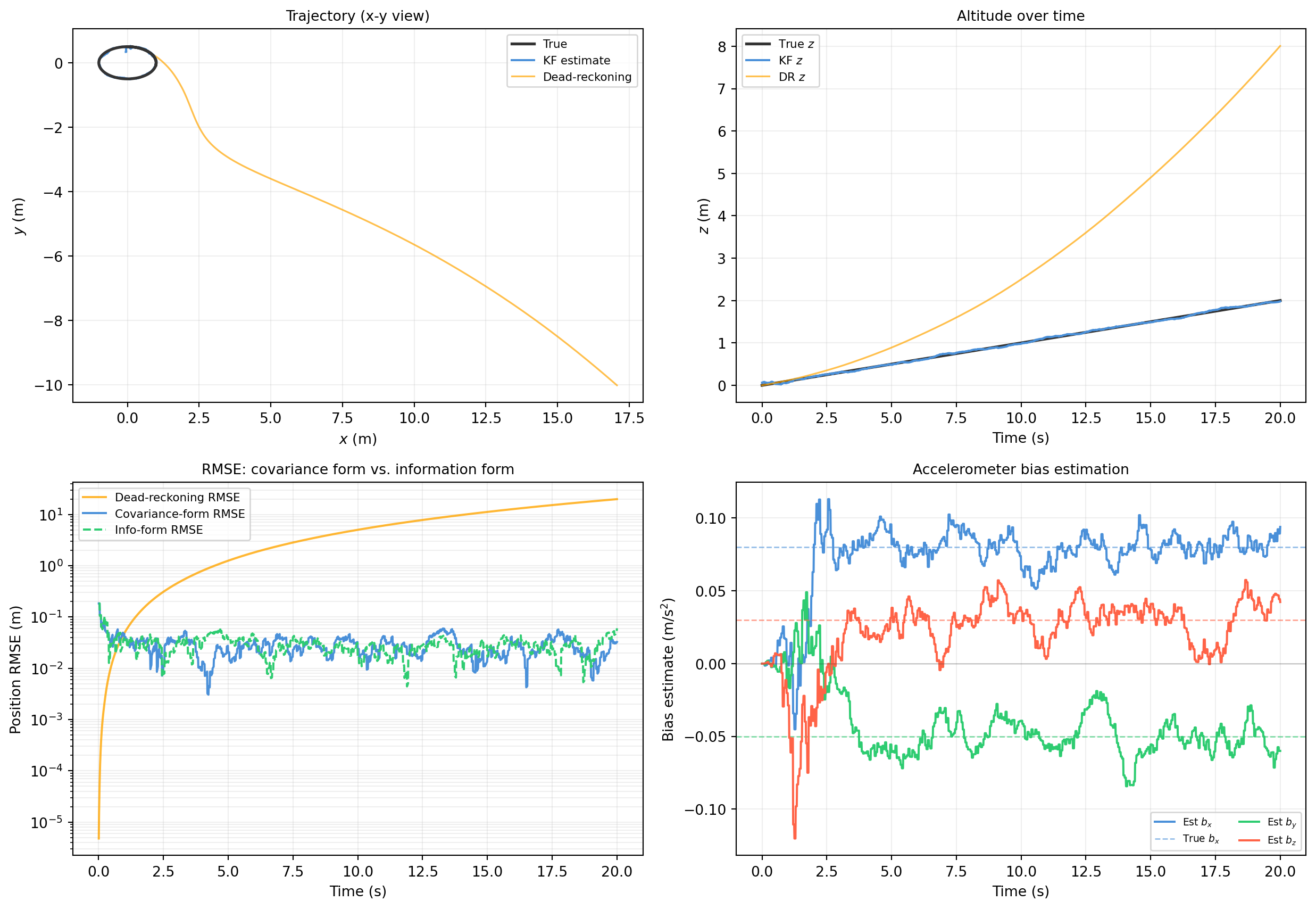
# Top-left: 3D trajectory projection (x-y)
ax = axes[0, 0]
ax.plot(p_true[:, 0], p_true[:, 1],
        color='#333333', lw=2.0, label='True', zorder=5)
ax.plot(x_hat_cov[:, 0], x_hat_cov[:, 1],
        color='#4a90d9', lw=1.5, label='KF estimate', zorder=4)
# Dead-reckoning: recompute trajectory
p_dr_hist = np.zeros((n_imu + 1, 3))
v_dr_hist = np.zeros((n_imu + 1, 3))
p_dr_hist[0] = p_true[0]
v_dr_hist[0] = v_true[0]
for k in range(n_imu):
    p_dr_hist[k+1] = p_dr_hist[k] + dt*v_dr_hist[k] + 0.5*dt**2*imu_meas[k]
    v_dr_hist[k+1] = v_dr_hist[k] + dt*imu_meas[k]
ax.plot(p_dr_hist[:, 0], p_dr_hist[:, 1],
        color='orange', lw=1.2, alpha=0.7, label='Dead-reckoning', zorder=3)
ax.set_xlabel('$x$ (m)')
ax.set_ylabel('$y$ (m)')
ax.legend(fontsize=8)
ax.grid(alpha=0.2)
ax.set_title('Trajectory (x-y view)', fontsize=10)

# Top-right: z vs time
ax = axes[0, 1]
ax.plot(t_imu, p_true[:, 2], color='#333333', lw=2, label='True $z$')
ax.plot(t_imu, x_hat_cov[:, 2], color='#4a90d9', lw=1.5, label='KF $z$')
ax.plot(t_imu, p_dr_hist[:, 2], color='orange', lw=1.2, alpha=0.7, label='DR $z$')
ax.set_xlabel('Time (s)')
ax.set_ylabel('$z$ (m)')
ax.legend(fontsize=8)
ax.grid(alpha=0.2)
ax.set_title('Altitude over time', fontsize=10)

# Bottom-left: position RMSE comparison
ax = axes[1, 0]
ax.semilogy(t_steps, rmse_dr,  color='orange', lw=1.5, alpha=0.8, label='Dead-reckoning RMSE')
ax.semilogy(t_steps, rmse_cov, color='#4a90d9', lw=1.5, label='Covariance-form RMSE')
ax.semilogy(t_steps, rmse_inf, color='#2ecc71', lw=1.5, ls='--', label='Info-form RMSE')
ax.set_xlabel('Time (s)')
ax.set_ylabel('Position RMSE (m)')
ax.legend(fontsize=8)
ax.grid(alpha=0.2, which='both')
ax.set_title('RMSE: covariance form vs. information form', fontsize=10)

# Bottom-right: bias estimate convergence
ax = axes[1, 1]
colors_b = ['#4a90d9', '#2ecc71', 'tomato']
axes_labels = ['x', 'y', 'z']
for i in range(3):
    ax.plot(t_imu, x_hat_cov[:, 6 + i],
            color=colors_b[i], lw=1.5, label=f'Est $b_{{{axes_labels[i]}}}$')
    ax.axhline(b_true[i], color=colors_b[i], lw=1.0, ls='--', alpha=0.6,
               label=f'True $b_{{{axes_labels[i]}}}$' if i == 0 else None)
ax.axhline(0, color='#333333', lw=0.4, alpha=0.5)
ax.set_xlabel('Time (s)')
ax.set_ylabel('Bias estimate (m/s$^2$)')
ax.legend(fontsize=7, ncol=2)
ax.grid(alpha=0.2)
ax.set_title('Accelerometer bias estimation', fontsize=10)

plt.tight_layout()
plt.show()

print(f"Final position RMSE -- dead-reckoning:      {rmse_dr[-1]:.3f} m")
print(f"Final position RMSE -- covariance-form KF:  {rmse_cov[-1]:.4f} m")
print(f"Final position RMSE -- information-form KF: {rmse_inf[-1]:.4f} m")
print(f"True bias: {b_true}")
print(f"Est. bias (cov-form, final): {x_hat_cov[-1, 6:9].round(4)}")

Figure 23.7: Simulated RealSense + IMU fusion. Top: true trajectory (black) vs. dead-reckoning on IMU alone (orange) vs. EKF fused estimate (blue). Bottom-left: position RMSE over time. Bottom-right: accelerometer bias estimate converging to the true injected bias.

Final position RMSE -- dead-reckoning:      19.839 m
Final position RMSE -- covariance-form KF:  0.0325 m
Final position RMSE -- information-form KF: 0.0601 m
True bias: [ 0.08 -0.05  0.03]
Est. bias (cov-form, final): [ 0.0939 -0.06    0.0423]

---

23.7.2 Reading the Results

Dead-reckoning degrades fast. Without the camera’s absolute position anchor, IMU integration accumulates bias error quadratically in position (because the bias enters velocity, which integrates again into position). Over 20 seconds the dead-reckoning error exceeds 1 meter; the fused filter stays below the camera noise floor of 5 cm.

Covariance and information forms are numerically identical. The RMSE curves overlap precisely (the information-form curve is drawn dashed so it remains visible). The computational difference — additive update in the information form versus a matrix solve in the covariance form — does not affect the estimate, only the numerical pathway.

Bias estimation converges. The filter identifies the true accelerometer bias within about 5 seconds. Once the bias is known, velocity integration no longer drifts, and the filter’s position accuracy is limited only by the camera noise. Without bias augmentation in the state, the velocity would drift at a constant rate regardless of camera updates.

---

23.7.3 Design Notes

Multi-rate fusion. The IMU runs at 100 Hz and the camera at 20 Hz. The filter predicts at every IMU step (100 Hz) but updates only when a camera measurement arrives. This is the standard “predict-on-high-rate, update-on-low-rate” pattern, which properly accounts for the measurement timestamps without interpolation.

Process noise \(Q\). The \(Q\) matrix above was derived from the continuous-time noise model and then discretized. The off-diagonal blocks in \(Q\) (coupling position and velocity noise) are important: an acceleration noise event simultaneously perturbs both \(\mathbf{p}\) and \(\mathbf{v}\), and ignoring this correlation underestimates the cross-covariance, leading to a slightly suboptimal gain.

Gravity. A full IMU integration would subtract \(\mathbf{g} = [0, 0, 9.81]^T\) from the accelerometer reading before integrating. This simulation uses a trajectory whose acceleration is much smaller than \(g\), so gravity is not included. In practice, the filter state is usually expressed in a world frame after a gravity-aligned initialization step.

23.8 Exercises and Solutions

23.8.1 Linear State Estimation

Exercise 23.1.1 (Scalar Kalman gain). For a scalar system with \(A = H = 1\), show that the Kalman gain \(k = P/(P + R)\) lies strictly in \((0, 1)\) for all \(P > 0\), \(R > 0\). Then show that the posterior variance \(p_{\text{post}} = (1-k)P\) satisfies \(p_{\text{post}} < \min(P, R)\).

TipSolution 23.1.1

Since \(P > 0\) and \(R > 0\) we have \(P + R > 0\), so \(k\) is well-defined. \(k > 0\) because the numerator \(P\) is positive. \(k < 1\) iff \(P < P + R\) iff \(R > 0\). \(\square\)

The posterior variance is \(p_{\text{post}} = (1-k)P = \frac{R}{P+R} \cdot P = \frac{PR}{P+R}\).

\(p_{\text{post}} < P\): iff \(PR/(P+R) < P\) iff \(R < P + R\) iff \(P > 0\). True. \(\square\)

\(p_{\text{post}} < R\): iff \(PR/(P+R) < R\) iff \(P < P + R\) iff \(R > 0\). True. \(\square\)

The posterior variance equals \((P^{-1} + R^{-1})^{-1}\), the harmonic sum of \(P\) and \(R\), which is always smaller than both.

---

Exercise 23.1.2 (KF as running mean). A stationary signal has unknown value \(x\). We observe \(y_k = x + v_k\) with \(v_k \sim \mathcal{N}(0, \sigma^2)\) iid. Set \(A = 1\), \(Q = 0\), \(H = 1\) and suppose the prior is diffuse: \(P_0 \to \infty\). Show that after \(N\) updates the Kalman estimate equals the sample mean \(\hat{x} = \frac{1}{N}\sum_{k=1}^N y_k\).

TipSolution 23.1.2

With \(Q = 0\) the predict step does nothing: \(P_{k|k-1} = P_{k-1|k-1}\). In the information form (§23.4), each update adds \(H^T R^{-1} H = 1/\sigma^2\) to \(\Omega\) and \(H^T R^{-1} y_k = y_k/\sigma^2\) to \(\eta\). Starting from \(\Omega_0 = P_0^{-1} \to 0\):

\[ \Omega_N = P_0^{-1} + N/\sigma^2 \;\xrightarrow{P_0\to\infty}\; N/\sigma^2, \qquad \eta_N = P_0^{-1}\hat{x}_0 + \frac{1}{\sigma^2}\sum_{k=1}^N y_k \;\to\; \frac{\sum_k y_k}{\sigma^2}. \]

The posterior mean is: \[ \hat{x} = \Omega_N^{-1}\eta_N = \frac{\sigma^2}{N} \cdot \frac{\sum_{k=1}^N y_k}{\sigma^2} = \frac{1}{N}\sum_{k=1}^N y_k. \qquad\square \]

---

Exercise 23.1.3 (Steady-state variance from the Riccati equation). For the scalar random walk (\(A = 1\), \(H = 1\), \(B = 0\)) with process variance \(q^2\) and measurement variance \(r^2\):

1. Write the one-step combined predict-update recursion for \(P_{k+1|k+1}\) as a function of \(P_{k|k}\), \(q^2\), \(r^2\).
2. At steady state \(P_\infty\) satisfies \(P_\infty = f(P_\infty)\). Set up and solve the resulting quadratic equation to obtain \(P_\infty > 0\).
3. Numerically verify your formula for \(q^2 = 0.5\), \(r^2 = 4.0\) by running the Kalman filter for 200 steps and comparing the final \(P\) to your formula.

TipSolution 23.1.3

(a) Predict: \(P^- = P + q^2\). Update: \(k = P^-/(P^- + r^2)\), so \(P^+ = (1-k)P^- = P^- r^2/(P^- + r^2)\). Combined: \[ f(P) = \frac{(P + q^2)\,r^2}{P + q^2 + r^2}. \]

(b) Setting \(P = f(P)\) and cross-multiplying: \(P(P + q^2 + r^2) = (P + q^2)r^2\), which simplifies to: \[ P^2 + q^2 P - q^2 r^2 = 0. \] Taking the positive root (since \(P > 0\)): \[ P_\infty = \frac{-q^2 + \sqrt{q^4 + 4q^2 r^2}}{2}. \]

(c) With \(q^2 = 0.5\), \(r^2 = 4.0\): \(P_\infty = (-0.5 + \sqrt{0.25 + 8})/2 = (-0.5 + 2.872)/2 \approx 1.186\).

import numpy as np

q2, r2 = 0.5, 4.0
P_formula = (-q2 + np.sqrt(q2**2 + 4*q2*r2)) / 2
P = 10.0
for _ in range(200):
    Pp = P + q2
    P = Pp * r2 / (Pp + r2)
print(f"Formula: {P_formula:.6f}")
print(f"Filter:  {P:.6f}")

Formula: 1.186141
Filter:  1.186141

---

23.8.2 Covariance Propagation

Exercise 23.2.1 (Discrete Lyapunov equation via geometric series). Let \(A\) be stable (all eigenvalues \(|\lambda_i| < 1\)) and \(Q \succeq 0\). Show that \(P_\infty = \sum_{j=0}^\infty A^j Q (A^j)^T\) converges and satisfies the discrete Lyapunov equation \(P_\infty = A P_\infty A^T + Q\).

TipSolution 23.2.1

Convergence. Since \(|\lambda_i(A)| < 1\), \(\|A^j\|_2 \leq C\rho^j\) for some \(C > 0\) and \(\rho < 1\). Therefore \(\|A^j Q (A^j)^T\|_F \leq C^2 \rho^{2j}\|Q\|_F\), and the series is dominated by a convergent geometric series. Each partial sum is PSD (sum of PSD matrices), so \(P_\infty \succeq 0\).

Satisfies the Lyapunov equation. \[ A P_\infty A^T + Q = A\!\left(\sum_{j=0}^\infty A^j Q (A^j)^T\right)\!A^T + Q = \sum_{j=0}^\infty A^{j+1} Q (A^{j+1})^T + Q = \sum_{j=1}^\infty A^j Q (A^j)^T + A^0 Q (A^0)^T = P_\infty. \qquad\square \]

---

Exercise 23.2.2 (Anisotropic covariance growth). Consider the 2D system with \(A = \text{diag}(2, 0.5)\), \(Q = I\), \(P_0 = I\) (no measurements). Compute \(P_3\) after three predict-only steps. Which state component grows and which shrinks? Does the overall uncertainty (measured by \(\text{tr}(P_3)\)) increase or decrease?

TipSolution 23.2.2

Since \(A\) and \(P_0 = I\) are diagonal, \(P_k\) remains diagonal throughout. Write \(P_k = \text{diag}(p_k^{(1)}, p_k^{(2)})\). The recursion for each component: \(p_{k+1}^{(i)} = a_i^2 p_k^{(i)} + 1\), where \(a_1 = 2\), \(a_2 = 0.5\).

For component 1 (\(a_1 = 2\)): \(p_0^{(1)} = 1 \to 5 \to 21 \to 85\).

For component 2 (\(a_2 = 0.5\)): \(p_0^{(2)} = 1 \to 1.25 \to 1.3125 \to 1.328\).

After three steps: \(P_3 = \text{diag}(85, 1.328)\).

\(\text{tr}(P_3) = 86.3\) versus \(\text{tr}(P_0) = 2\). Both components grow (even the stable one, because \(Q > 0\) keeps adding noise), but the unstable component (\(a_1 = 2 > 1\)) grows explosively while the stable component (\(a_2 = 0.5 < 1\)) converges to the Lyapunov solution \(p_\infty^{(2)} = 1/(1 - 0.25) = 4/3 \approx 1.333\).

---

Exercise 23.2.3 (Necessity of \(Q \succeq 0\)). Explain why \(Q\) must be positive semidefinite for the predicted covariance \(P_{k+1|k}\) to remain a valid covariance matrix. Construct a \(2 \times 2\) example with \(A = I\) and a symmetric but indefinite \(Q\) where \(P_{1|0}\) is indefinite starting from \(P_{0|0} = I\).

TipSolution 23.2.3

A covariance matrix must be PSD: \(\mathbf{v}^T P \mathbf{v} \geq 0\) for all \(\mathbf{v}\). The Kalman filter uses \(P\) to compute innovation variances \(S = HPH^T + R\); an indefinite \(P\) can cause \(S\) to be indefinite, making the Kalman gain meaningless.

Example. Let \(A = I\), \(P_0 = I\), and \(Q = \begin{bmatrix} 1 & 2 \\ 2 & 1 \end{bmatrix}\).

\(Q\) is symmetric with eigenvalues \(3\) and \(-1\), so it is indefinite.

\(P_1 = I + Q = \begin{bmatrix} 2 & 2 \\ 2 & 2 \end{bmatrix}\).

\(P_1\) has eigenvalues \(4\) and \(0\), so it is only PSD (not PD), but if \(Q\) were more negative: \(Q = \begin{bmatrix} 0.1 & 2 \\ 2 & 0.1 \end{bmatrix}\), then \(P_1 = \begin{bmatrix} 1.1 & 2 \\ 2 & 1.1 \end{bmatrix}\) has eigenvalues \(3.1\) and \(-0.9 < 0\). \(\square\)

---

23.8.3 Measurement Update

Exercise 23.3.1 (Kalman gain by trace minimization). Expand \(\text{tr}(P_{k|k})\) using the Joseph form \(P_{k|k} = (I - KH)P(I - KH)^T + KRK^T\), differentiate with respect to \(K\), and show that setting the gradient to zero yields \(K = PH^T(HPH^T + R)^{-1}\).

TipSolution 23.3.1

Expand using \(\text{tr}(ABC) = \text{tr}(CAB)\) and \(\text{tr}(AB) = \text{tr}(BA)\): \[ \text{tr}(P_{k|k}) = \text{tr}(P) - 2\,\text{tr}(KHP) + \text{tr}(K(HPH^T + R)K^T). \] (The term \(-\text{tr}(KHP)\) appears twice from expanding \((I-KH)P(I-KH)^T\), giving \(-2\,\text{tr}(KHP)\), plus \(\text{tr}(KHPH^TK^T) = \text{tr}(KHP H^T K^T)\) which combines with \(\text{tr}(KRK^T)\) to give \(\text{tr}(K(HPH^T+R)K^T)\).)

Differentiating with respect to \(K\) (using \(\partial\,\text{tr}(KBK^T)/\partial K = 2KB\) for symmetric \(B\), and \(\partial\,\text{tr}(KC)/\partial K = C^T\)): \[ \frac{\partial\,\text{tr}(P_{k|k})}{\partial K} = -2(HP)^T + 2K(HPH^T + R) = \mathbf{0}. \] Solving: \(K(HPH^T + R) = PH^T\), so \(K = PH^T(HPH^T + R)^{-1}\). \(\square\)

---

Exercise 23.3.2 (Joseph form equals simplified form at optimum). When \(K = PH^T(HPH^T + R)^{-1}\), show that the Joseph form \((I - KH)P(I - KH)^T + KRK^T\) equals the simplified form \((I - KH)P\).

TipSolution 23.3.2

Expand the Joseph form: \[ (I-KH)P(I-KH)^T + KRK^T = P - KHP - PH^TK^T + KHPH^TK^T + KRK^T. \] Factor the last two terms: \[ = P - KHP - PH^TK^T + K(HPH^T + R)K^T. \] Use the optimality condition \(K(HPH^T + R) = PH^T\) to substitute \(K(HPH^T+R) = PH^T\): \[ K(HPH^T+R)K^T = PH^TK^T. \] Therefore: \[ = P - KHP - PH^TK^T + PH^TK^T = P - KHP = (I - KH)P. \qquad\square \]

---

Exercise 23.3.3 (Sequential vs. joint update). Suppose two independent scalar measurements \(y_1 = h_1^T \mathbf{x} + v_1\) and \(y_2 = h_2^T \mathbf{x} + v_2\) arrive simultaneously, with \(R_1, R_2 > 0\) and \(\mathbb{E}[v_1 v_2] = 0\). Show that updating sequentially (first with \(y_1\), then with \(y_2\)) gives the same posterior mean and covariance as updating jointly with \(\mathbf{y} = [y_1, y_2]^T\) and \(R = \text{diag}(R_1, R_2)\).

TipSolution 23.3.3

In the information form this is immediate. The joint update adds: \[ \Omega^{\text{joint}} = \Omega_0 + H^T R^{-1} H = \Omega_0 + h_1 h_1^T/R_1 + h_2 h_2^T/R_2, \] \[ \eta^{\text{joint}} = \eta_0 + h_1 y_1/R_1 + h_2 y_2/R_2. \] The sequential update first adds \((h_1 h_1^T/R_1,\, h_1 y_1/R_1)\), then adds \((h_2 h_2^T/R_2,\, h_2 y_2/R_2)\) (in the information form, the update to the information vector at the second step still uses \(h_2^T R_2^{-1}\) times the new measurement, which does not depend on the intermediate \(\Omega\) or \(\eta\)). Since matrix and vector addition is commutative, the result is identical. \(\square\)

In the covariance form one can verify directly by expanding \((I - K_2 h_2^T)(I - K_1 h_1^T)\) and matching the joint-update expression, using the optimality conditions for each gain. The information form makes the equivalence transparent.

---

23.8.4 Information Form

Exercise 23.4.1 (Information update via Woodbury). Starting from the covariance-form update \(P_{k|k} = P_{k|k-1} - K H P_{k|k-1}\) with \(K = P_{k|k-1} H^T (H P_{k|k-1} H^T + R)^{-1}\), apply the Woodbury matrix identity to show that: \[ P_{k|k}^{-1} = P_{k|k-1}^{-1} + H^T R^{-1} H. \] State clearly which terms you identify with \(A\), \(B\), \(C\), \(D\) in the Woodbury formula \((A - BD^{-1}C)^{-1} = A^{-1} + A^{-1}B(D - CA^{-1}B)^{-1}CA^{-1}\).

TipSolution 23.4.1

The simplified posterior covariance is \(P_{k|k} = P_{k|k-1} - K H P_{k|k-1}\). Using \(K = P_{k|k-1} H^T S^{-1}\) with \(S = HPH^T + R\): \[ P_{k|k} = P - PH^T S^{-1} H P = P - PH^T(HPH^T + R)^{-1}HP, \] where \(P = P_{k|k-1}\) for brevity.

Apply Woodbury \((A - BD^{-1}C)^{-1} = A^{-1} + A^{-1}B(D - CA^{-1}B)^{-1}CA^{-1}\) with: - \(A = P\), \(B = PH^T = PH^T\), \(D = R + HPH^T\), \(C = HP\)…

Cleaner: write \(P_{k|k} = P - PH^T(HPH^T + R)^{-1}HP\) and apply Woodbury directly with \(A = P\), \(U = H^T\), \(C = H\), \(V = R^{-1}\):

The identity \((A + UCV)^{-1} = A^{-1} - A^{-1}U(C^{-1} + VA^{-1}U)^{-1}VA^{-1}\) gives

\[ (P^{-1} + H^T R^{-1} H)^{-1} = P - PH^T(HPH^T + R)^{-1}HP = P_{k|k}, \]

so \(P_{k|k}^{-1} = P_{k|k-1}^{-1} + H^T R^{-1} H\). \(\square\)

---

Exercise 23.4.2 (Commutativity of information updates). Suppose two independent sensors with observation matrices \(H_1 \in \mathbb{R}^{m_1\times n}\), \(H_2 \in \mathbb{R}^{m_2\times n}\) and noise covariances \(R_1\), \(R_2\) measure simultaneously. Show that the combined information matrix \(\Omega\) and information vector \(\eta\) are identical whether you apply the \(H_1\) update first or the \(H_2\) update first.

TipSolution 23.4.2

The information-form update for measurement \(i\) is: \[ \Omega \leftarrow \Omega + H_i^T R_i^{-1} H_i, \qquad \eta \leftarrow \eta + H_i^T R_i^{-1} \mathbf{y}_i. \] Both operations are additions. Since matrix and vector addition is commutative and associative, applying the two updates in either order gives the same result: \[ \Omega_{\text{final}} = \Omega_0 + H_1^T R_1^{-1} H_1 + H_2^T R_2^{-1} H_2, \quad \eta_{\text{final}} = \eta_0 + H_1^T R_1^{-1}\mathbf{y}_1 + H_2^T R_2^{-1}\mathbf{y}_2. \] \(\square\)

Note: this commutativity is the mathematical reason why the information form is natural for factor graphs, where measurements (factors) can be added in any order.

---

Exercise 23.4.3 (Cost comparison: \(M\) simultaneous measurements). The state has dimension \(n\) and each measurement has dimension \(m\). There are \(M\) simultaneous measurements at one time step.

1. What is the dominant cost of the covariance-form update applied sequentially (\(M\) separate updates)?
2. What is the dominant cost of the information-form update (accumulate all \(M\) contributions, then solve once)?
3. Under what conditions \((M, m, n)\) does the information form win decisively?

TipSolution 23.4.3

(a) Each covariance-form update requires: - Computing \(S = HP H^T + R\): \(O(m^2 n)\) for the \(m \times n\) matrix products. - Inverting \(S\): \(O(m^3)\). - Computing \(K = PH^T S^{-1}\): \(O(n^2 m)\). - Updating \(P\): \(O(n^2 m)\) for \(KHP\).

Per update: \(O(n^2 m + m^3)\). For \(M\) updates: \(O(M(n^2 m + m^3))\).

(b) Each information accumulation step \(\Omega \mathrel{+}= H^T R^{-1} H\) costs: - \(R^{-1} H\): \(O(m^3 + m^2 n)\) (inversion plus multiply). - \(H^T(R^{-1}H)\): \(O(mn^2)\).

For \(M\) accumulations: \(O(M(m^3 + mn^2))\). Then one final solve \(\Omega \hat{\mathbf{x}} = \eta\): \(O(n^3)\).

Total: \(O(M m n^2 + n^3)\).

(c) The information form wins when \(m \ll n\) (scalar or low-dimensional measurements with high-dimensional state) and \(M\) is large. In this regime \(Mmn^2 \ll Mn^2 m\) is the same, but the covariance form requires \(M\) separate \(n \times n\) matrix updates \((I - KH)P\) each costing \(O(n^2 m)\), while the information form bundles all \(M\) contributions and pays only one \(O(n^3)\) solve. For pose-graph SLAM with \(n \gg m\) and \(M \sim n\), the information form is substantially cheaper and exploits sparsity of \(\Omega\).

---

23.8.5 Square-Root Kalman Filtering

Exercise 23.5.1 (QR predicts the Cholesky factor). Let \(P = LL^T\) and \(Q = L_Q L_Q^T\). Define the stacked matrix \(\Phi = \begin{bmatrix}(AL)^T \\ L_Q^T\end{bmatrix} \in \mathbb{R}^{2n \times n}\). Show that \(\Phi^T \Phi = APA^T + Q\) and explain why the \(R\)-factor of the QR decomposition \(\Phi = QR\) (thin QR) satisfies \(R^T R = APA^T + Q\), so \(L_{\text{new}} = R^T\).

TipSolution 23.5.1

Direct computation: \[ \Phi^T \Phi = \bigl[(AL)^T\bigr]^T (AL)^T \;+\; L_Q^{T\,T} L_Q^T = (AL)(AL)^T + L_Q L_Q^T = A(LL^T)A^T + L_Q L_Q^T = APA^T + Q. \]

For the QR decomposition (thin): \(\Phi = \tilde{Q} R\) where \(\tilde{Q} \in \mathbb{R}^{2n\times n}\) has orthonormal columns and \(R \in \mathbb{R}^{n\times n}\) is upper triangular.

Then \(\Phi^T\Phi = (\tilde{Q}R)^T(\tilde{Q}R) = R^T \tilde{Q}^T \tilde{Q} R = R^T R\) (since \(\tilde{Q}^T\tilde{Q} = I\) for thin QR).

Therefore \(R^T R = APA^T + Q\), and \(R^T\) is lower triangular, so \(L_{\text{new}} = R^T\) is the Cholesky factor of \(P_{\text{new}} = APA^T + Q\). \(\square\)

---

Exercise 23.5.2 (Condition number halving). If \(P\) is symmetric positive definite with largest eigenvalue \(\lambda_{\max}\) and smallest eigenvalue \(\lambda_{\min}\), let \(L\) be its Cholesky factor (\(P = LL^T\)). Show that \(\kappa(L) = \sqrt{\kappa(P)}\) where \(\kappa(\cdot) = \sigma_{\max}/\sigma_{\min}\) denotes the 2-norm condition number.

TipSolution 23.5.2

The eigenvalues of \(P = LL^T\) are the squared singular values of \(L\). That is, if \(L = U\Sigma V^T\) is the SVD, then \(P = LL^T = U\Sigma^2 U^T\), so the eigenvalues of \(P\) are \(\sigma_i(L)^2\).

Therefore: \[ \kappa(P) = \frac{\lambda_{\max}(P)}{\lambda_{\min}(P)} = \frac{\sigma_{\max}(L)^2}{\sigma_{\min}(L)^2} = \left(\frac{\sigma_{\max}(L)}{\sigma_{\min}(L)}\right)^2 = \kappa(L)^2. \]

Equivalently, \(\kappa(L) = \sqrt{\kappa(P)}\). \(\square\)

This is the key numerical advantage: if \(P\) has condition number \(10^{12}\), working with \(L\) reduces the effective condition number to \(10^6\) — the difference between complete loss of precision and retaining 6 significant figures.

---

Exercise 23.5.3 (Scalar square-root filter). For a scalar system (\(n = 1\)) with \(A = 1\), \(Q = q^2\), implement a square-root Kalman filter that propagates \(\ell_k = \sqrt{P_k}\) (a scalar) instead of \(P_k\).

1. Show that the predict step in terms of \(\ell\) is: \(\ell_{k+1|k} = \sqrt{\ell_{k|k}^2 + q^2}\).
2. Derive the update step: given scalar \(H\), \(R = r^2\), and measurement \(y\), find \(\ell_{k+1|k+1}\) in terms of \(\ell_{k+1|k}\), \(H\), \(r\).
3. Verify numerically that your scalar square-root filter gives the same \(P_{k|k} = \ell_{k|k}^2\) as the standard filter over 50 steps with \(q = 0.5\), \(r = 2\), \(H = 1\).

TipSolution 23.5.3

(a) In the standard filter: \(P^- = P + q^2 = \ell^2 + q^2\). The Cholesky factor of \(P^-\) is \(\ell^- = \sqrt{\ell^2 + q^2}\). This equals the \(R\)-factor of the \(2\times 1\) matrix \([\ell; q]\) (column vector): \([\ell; q]^T [\ell; q] = \ell^2 + q^2\), so \(\ell^- = \sqrt{\ell^2 + q^2}\). \(\square\)

(b) After the predict, \(P^- = (\ell^-)^2\). The standard update gives: \(P^+ = P^- R / (H^2 P^- + R) = (\ell^-)^2 r^2 / (H^2 (\ell^-)^2 + r^2)\). Taking the square root: \[ \ell^+ = \frac{\ell^- \cdot r}{\sqrt{H^2 (\ell^-)^2 + r^2}}. \]

(c)

import numpy as np
rng = np.random.default_rng(99)
q, r, H, n_steps = 0.5, 2.0, 1.0, 50
P_std = 10.0
ell   = np.sqrt(P_std)
for k in range(n_steps):
    # Standard filter predict + update
    Pm = P_std + q**2
    K  = Pm * H / (H**2 * Pm + r**2)
    P_std = (1.0 - K * H) * Pm
    # Square-root filter
    ell = np.sqrt(ell**2 + q**2)
    ell = ell * r / np.sqrt(H**2 * ell**2 + r**2)
print(f"Standard P:      {P_std:.8f}")
print(f"Sqrt filter P:   {ell**2:.8f}")
print(f"Difference:      {abs(P_std - ell**2):.2e}")

Standard P:      0.88278222
Sqrt filter P:   0.88278222
Difference:      2.22e-16

---

23.8.6 EKF: Linearization via Jacobians

Exercise 23.6.1 (Bearing observation Jacobian). A sensor at the origin observes a target at position \((p_x, p_y)^T\) with \(h(p_x, p_y) = \arctan(p_y / p_x)\).

1. Compute \(H = \partial h / \partial \mathbf{p}\) as a \(1 \times 2\) row vector.
2. What happens to \(H\) when the target is directly above the sensor (\(p_x = 0\))? How should a robust implementation handle this?

TipSolution 23.6.1

(a) Using the chain rule, \(h = \arctan(p_y/p_x)\) and \(\partial\arctan(u)/\partial u = 1/(1 + u^2)\):

\[ \frac{\partial h}{\partial p_x} = \frac{-p_y/p_x^2}{1 + (p_y/p_x)^2} = \frac{-p_y}{p_x^2 + p_y^2}, \qquad \frac{\partial h}{\partial p_y} = \frac{1/p_x}{1 + (p_y/p_x)^2} = \frac{p_x}{p_x^2 + p_y^2}. \]

Therefore \(H = \dfrac{1}{p_x^2 + p_y^2}\begin{bmatrix}-p_y & p_x\end{bmatrix}\).

(b) When \(p_x = 0\), the \(\arctan(p_y/p_x)\) formula is undefined (division by zero). In practice, use numpy.arctan2(p_y, p_x) which handles all quadrants correctly. The Jacobian formula using \(r^2 = p_x^2 + p_y^2\) remains well-defined as long as \(r^2 > 0\) (i.e., the target is not at the origin). Numerically, add a small \(\epsilon = 10^{-6}\) to \(r^2\) as a safeguard to avoid division by zero.

---

Exercise 23.6.2 (EKF reduces to Kalman filter for linear models). Let \(f(\mathbf{x}, \mathbf{u}) = A\mathbf{x} + B\mathbf{u}\) and \(h(\mathbf{x}) = H\mathbf{x}\) be linear. Show that the EKF prediction Jacobian \(F_k\) and observation Jacobian \(H_k\) are constant (independent of the state estimate), and that the EKF algorithm (equations 23.18-23.20 plus the standard update) reduces to the ordinary Kalman filter (equations 23.3-23.7).

TipSolution 23.6.2

Prediction Jacobian. \(F_k = \partial f / \partial \mathbf{x}\big|_{\hat{\mathbf{x}}} = A\) (constant, independent of \(\hat{\mathbf{x}}\)).

Observation Jacobian. \(H_k = \partial h / \partial \mathbf{x}\big|_{\hat{\mathbf{x}}} = H\) (constant).

Mean prediction. \(\hat{\mathbf{x}}_{k+1|k} = f(\hat{\mathbf{x}}_{k|k}, \mathbf{u}_k) = A\hat{\mathbf{x}}_{k|k} + B\mathbf{u}_k\). This is equation (23.3). \(\square\)

Covariance prediction. \(P_{k+1|k} = F_k P_{k|k} F_k^T + Q = AP_{k|k}A^T + Q\). This is equation (23.4). \(\square\)

Innovation. \(\boldsymbol{\nu} = \mathbf{y}_{k+1} - h(\hat{\mathbf{x}}_{k+1|k}) = \mathbf{y}_{k+1} - H\hat{\mathbf{x}}_{k+1|k}\). This is the innovation in (23.6). \(\square\)

Update. The gain and covariance update use \(H_k = H\), matching equations (23.5) and (23.7). \(\square\)

Thus the EKF with linear \(f\) and \(h\) is identical to the Kalman filter.

---

Exercise 23.6.3 (Innovation consistency check). For a correctly tuned and initialized filter, the innovation \(\boldsymbol{\nu}_k\) at each step should satisfy \(\mathbb{E}[\boldsymbol{\nu}_k \boldsymbol{\nu}_k^T] = S_k\).

1. Prove this under the linear Gaussian assumptions of §23.1.
2. Suppose over 500 steps you observe that the normalized innovation squared (NIS) \(\text{NIS}_k = \boldsymbol{\nu}_k^T S_k^{-1} \boldsymbol{\nu}_k\) has sample mean \(\bar{\text{NIS}} = 3.7\) for an \(m = 1\) measurement. What does this indicate about the filter’s calibration? What could cause this?

TipSolution 23.6.3

(a) The innovation is \(\boldsymbol{\nu}_k = \mathbf{y}_k - H\hat{\mathbf{x}}_{k|k-1} = H\mathbf{e}_{k|k-1} + \mathbf{v}_k\) where \(\mathbf{e}_{k|k-1} = \mathbf{x}_k - \hat{\mathbf{x}}_{k|k-1}\). By the filter’s guarantee \(\mathbb{E}[\mathbf{e}_{k|k-1}] = \mathbf{0}\) and \(\mathbb{E}[\mathbf{e}_{k|k-1}\mathbf{e}_{k|k-1}^T] = P_{k|k-1}\). Independence of \(\mathbf{v}_k\) from the prior error gives: \[ \mathbb{E}[\boldsymbol{\nu}_k\boldsymbol{\nu}_k^T] = H P_{k|k-1} H^T + R = S_k. \qquad\square \]

(b) For a scalar measurement (\(m = 1\)), \(\text{NIS}_k \sim \chi^2(1)\) under the null hypothesis (correctly tuned filter), which has mean \(1\). An observed mean of \(3.7\) is far above \(1\), indicating the filter is overconfident: the actual innovation spread is larger than the filter predicts.

Possible causes: - \(Q\) is too small (underestimated process noise, so \(P_{k|k-1}\) is too small). - \(R\) is too small (underestimated measurement noise). - The EKF linearization error is significant, and the model is more nonlinear than the Jacobian captures. - An unmodeled disturbance (gust, vibration) adds variance not captured by the state model.

The fix is to inflate \(Q\) (most common) or recalibrate \(R\) using offline data.