27  Appendix B: Matrix Factorization Summary

27.1 Matrix Factorization Summary

Every major matrix factorization decomposes a matrix into structured factors that expose a different geometric or algebraic property. Knowing which factorization to reach for – and why – is as important as knowing the API.

---

27.1.1 At a Glance

Factorization	Form	Requirement	Cost	Primary uses
LU	\(PA = LU\)	Square	\(O(n^3)\)	Solve \(Ax = b\), compute det
Cholesky	\(A = LL^T\)	Symmetric PD	\(\tfrac{1}{2}O(n^3)\)	Kalman filter, multivariate sampling
QR	\(A = QR\)	Any	\(O(mn^2)\)	Least squares, eigenvalue algorithms
Eigendecomposition	\(A = P\Lambda P^{-1}\)	Square, diagonalizable	\(O(n^3)\)	Dynamics, stability, PageRank
Spectral	\(A = Q\Lambda Q^T\)	Symmetric	\(O(n^3)\)	PCA, quadratic forms, Hessians
SVD	\(A = U\Sigma V^T\)	Any	\(O(mn^2)\)	Low-rank approx, pseudoinverse, PCA

import numpy as np
import matplotlib.pyplot as plt
import matplotlib.patches as mpatches
import scipy.linalg

rng = np.random.default_rng(42)
n = 6

A_sq = rng.standard_normal((n, n))
A_sq = A_sq @ A_sq.T + n * np.eye(n)   # shape (n, n)  SPD

P_mat, L, U = scipy.linalg.lu(A_sq)             # PA = LU
L_cho = np.linalg.cholesky(A_sq)                # A = L L^T
Q_qr, R_qr = np.linalg.qr(A_sq)                # A = Q R
vals, P_eig = np.linalg.eigh(A_sq)              # symmetric -- spectral
Lam = np.diag(vals)                              # shape (n, n)
U_svd, s, Vt = np.linalg.svd(A_sq, full_matrices=False)  # shape (n,)

threshold = 1e-10
patterns = [
    (np.abs(L) > threshold,        'L\n(lower)'),
    (np.abs(U) > threshold,        'U\n(upper)'),
    (np.abs(L_cho) > threshold,    'L\n(Cholesky)'),
    (np.abs(Q_qr) > threshold,     'Q\n(orthogonal)'),
    (np.abs(R_qr) > threshold,     'R\n(upper)'),
    (np.abs(P_eig) > threshold,    'P\n(eigenvecs)'),
    (np.abs(Lam) > threshold,      'Lambda\n(diagonal)'),
    (np.abs(U_svd) > threshold,    'U\n(left sv)'),
    (np.abs(Vt) > threshold,       'V^T\n(right sv)'),
]

fig, axes = plt.subplots(1, 9, figsize=(13, 2.0))
for ax, (pat, label) in zip(axes, patterns):
    ax.imshow(pat, cmap='Blues', vmin=0, vmax=1, aspect='auto')
    ax.set_title(label, fontsize=7.5)
    ax.set_xticks([])
    ax.set_yticks([])

plt.suptitle('Factor sparsity patterns (n = 6)', fontsize=9, y=1.03)
plt.tight_layout()
plt.show()

Figure 27.1: Sparsity patterns of the factor matrices produced by each decomposition for a 6x6 example. Dark cells are non-zero entries; light cells are structural zeros. L (lower triangular), U (upper triangular), Q (orthogonal – dense), R (upper triangular), P (eigenvector matrix – dense), and U/V^T (singular vector matrices – dense).

---

27.2 LU Decomposition

Form: \(PA = LU\)

Gaussian elimination with partial pivoting factors a square matrix \(A\) into a permutation matrix \(P\), a unit lower-triangular matrix \(L\) (ones on diagonal), and an upper-triangular matrix \(U\).

27.2.1 Structure

Factor	Shape	Properties
\(P\)	\((n, n)\)	Permutation; \(P^T = P^{-1}\)
\(L\)	\((n, n)\)	Lower triangular; diagonal entries all 1
\(U\)	\((n, n)\)	Upper triangular; diagonal entries are pivots

The factorization always exists for any square matrix (no symmetry or positive-definiteness required). After factoring, each additional right-hand side costs \(O(n^2)\) via forward and back substitution.

---

27.2.2 API

Call	Description
np.linalg.solve(A, b)	Solve once; computes LU internally
scipy.linalg.lu_factor(A)	Return packed (lu, piv)
scipy.linalg.lu_solve((lu, piv), b)	Solve for each RHS using stored LU
scipy.linalg.lu(A)	Return explicit (P, L, U) matrices

import numpy as np
import scipy.linalg

rng = np.random.default_rng(0)
n = 4
A = rng.standard_normal((n, n))     # shape (4, 4)  general square
B = rng.standard_normal((n, 3))     # shape (4, 3)  multiple right-hand sides

# Factor once
lu, piv = scipy.linalg.lu_factor(A)        # packed representation

# Solve three right-hand sides cheaply
X = scipy.linalg.lu_solve((lu, piv), B)    # shape (4, 3)
print(f"||AX - B|| = {np.linalg.norm(A @ X - B):.2e}")

# Inspect factors explicitly
P, L, U = scipy.linalg.lu(A)              # P shape (4,4), L shape (4,4), U shape (4,4)
print(f"||PA - LU|| = {np.linalg.norm(P @ A - L @ U):.2e}")
print(f"L diagonal (all 1): {np.diag(L).round(4)}")
print(f"U diagonal (pivots): {np.diag(U).round(4)}")

||AX - B|| = 6.03e-16
||PA - LU|| = 1.16e-16
L diagonal (all 1): [1. 1. 1. 1.]
U diagonal (pivots): [-2.325  -1.1992  1.5065 -0.4487]

---

27.2.3 Determinant and Singular Systems

Once LU is available, the determinant is the product of the \(U\) diagonal (times the permutation sign), without a separate \(O(n^3)\) computation:

import numpy as np
import scipy.linalg

rng = np.random.default_rng(1)
A = rng.standard_normal((5, 5))   # shape (5, 5)

lu, piv = scipy.linalg.lu_factor(A)

# Sign of permutation: count swaps in piv
n = A.shape[0]
sign = (-1) ** int(np.sum(piv != np.arange(n)))
det_fast = sign * np.prod(np.diag(lu))
det_ref  = np.linalg.det(A)
print(f"det (fast): {det_fast:.6f}")
print(f"det (ref) : {det_ref:.6f}")

det (fast): 1.658587
det (ref) : 1.658587

scipy.linalg.lu_factor returns piv as a 1-D array of pivot indices used by LAPACK’s dgetrf, not a full permutation matrix. Use scipy.linalg.lu(A) when you need \(P\), \(L\), \(U\) as separate arrays.

---

27.2.4 Numerical Properties

Property	Value
Stability	Backward stable with partial pivoting
Condition sensitivity	\(\kappa(A) = \|A\| \cdot \|A^{-1}\|\) governs error
Memory	In-place; \(L\) and \(U\) share the storage of lu
Fails	Singular matrix (zero pivot encountered)

When the condition number \(\kappa(A)\) is large, small perturbations in \(b\) produce large changes in \(x\). Check np.linalg.cond(A) before trusting the solution.

---

27.3 Cholesky Decomposition

Form: \(A = LL^T\) (or equivalently \(A = U^T U\) with an upper triangular \(U\))

Cholesky factors a symmetric positive definite (SPD) matrix into a lower triangular matrix \(L\) whose diagonal entries are positive. It requires roughly half the floating-point operations of LU and is numerically very stable.

27.3.1 Structure

Factor	Shape	Properties
\(L\)	\((n, n)\)	Lower triangular; positive diagonal

Existence and uniqueness are guaranteed if and only if \(A\) is SPD. In practice, a failed Cholesky is the cheapest way to test whether a matrix is positive definite.

---

27.3.2 API

Call	Description
np.linalg.cholesky(A)	Return lower triangular \(L\); raises LinAlgError if not PD
scipy.linalg.cho_factor(A)	Return packed (c, lower) for repeated solves
scipy.linalg.cho_solve((c, lower), b)	Solve each RHS with stored Cholesky

import numpy as np
import scipy.linalg

rng = np.random.default_rng(0)
n = 5
A = rng.standard_normal((n, n))      # shape (5, 5)
A = A @ A.T + n * np.eye(n)          # shape (5, 5)  SPD
b = rng.standard_normal((n,))        # shape (5,)

# Single solve
L = np.linalg.cholesky(A)            # shape (5, 5)  lower triangular
print(f"||LL^T - A|| = {np.linalg.norm(L @ L.T - A):.2e}")
print(f"L diagonal (positive): {np.diag(L).round(4)}")

# Pre-factor for multiple right-hand sides
c, lower = scipy.linalg.cho_factor(A)         # packed Cholesky
x = scipy.linalg.cho_solve((c, lower), b)     # shape (5,)
print(f"||Ax - b||   = {np.linalg.norm(A @ x - b):.2e}")

||LL^T - A|| = 2.88e-15
L diagonal (positive): [2.3961 3.1016 3.4962 2.5086 2.8318]
||Ax - b||   = 2.31e-16

---

27.3.3 Applications in the Book

Sampling from a multivariate Gaussian \(\mathcal{N}(\mu, \Sigma)\):

If \(\Sigma = LL^T\), then \(x = \mu + L z\) where \(z \sim \mathcal{N}(0, I)\) produces samples from \(\mathcal{N}(\mu, \Sigma)\).

import numpy as np

rng = np.random.default_rng(7)
n_dim, n_samples = 3, 10000

# Covariance matrix and mean
Sigma = np.array([[2.0, 0.8, 0.3],
                  [0.8, 1.5, 0.1],
                  [0.3, 0.1, 1.0]])    # shape (3, 3)  SPD
mu    = np.array([1.0, 2.0, 0.5])     # shape (3,)

L = np.linalg.cholesky(Sigma)         # shape (3, 3)

z = rng.standard_normal((n_dim, n_samples))    # shape (3, 10000)
samples = mu[:, np.newaxis] + L @ z            # shape (3, 10000)

# Verify: empirical covariance should match Sigma
Sigma_emp = np.cov(samples)            # shape (3, 3)
print(f"Max error in recovered covariance: {np.abs(Sigma_emp - Sigma).max():.4f}")

Max error in recovered covariance: 0.0404

Kalman filter covariance update uses Cholesky for numerically stable square-root forms. Sparse SLAM solves the normal equations via sparse Cholesky (via scikit-sparse or cholmod).

---

27.3.4 Numerical Properties

Property	Value
Stability	Highly stable; no pivoting needed
Cost	\(\approx \frac{1}{3} n^3\) FLOPs (half of LU)
Failure mode	Raises np.linalg.LinAlgError if matrix is not PD
Near-singular case	Add small ridge A + eps * np.eye(n) before factoring

Diagonal check: np.all(np.diag(L) > 0) confirms positive definiteness after a successful Cholesky.

---

27.4 QR Decomposition

Form: \(A = QR\)

QR factors any \(m \times n\) matrix (\(m \ge n\)) into an orthogonal (or unitary) matrix \(Q\) and an upper-triangular matrix \(R\).

27.4.1 Thin vs Full QR

Mode	\(Q\) shape	\(R\) shape	When to use
Thin (economy)	\((m, n)\)	\((n, n)\)	Least squares, numerical linear algebra
Full	\((m, m)\)	\((m, n)\)	Completing orthonormal bases, null space

In the thin form, \(Q\) has orthonormal columns (\(Q^T Q = I_n\)) but is not square, so \(Q Q^T \ne I_m\). In the full form, \(Q\) is square and orthogonal (\(Q^T Q = Q Q^T = I_m\)).

---

27.4.2 API

Call	Description
np.linalg.qr(A)	Thin QR by default; returns (Q, R)
np.linalg.qr(A, mode='complete')	Full QR; \(Q\) is square \((m, m)\)
np.linalg.qr(A, mode='r')	\(R\) only (faster when \(Q\) not needed)
scipy.linalg.qr(A, pivoting=True)	Column-pivoted QR; reveals rank

import numpy as np

rng = np.random.default_rng(0)
m, n = 6, 4
A = rng.standard_normal((m, n))      # shape (6, 4)

# Thin QR
Q, R = np.linalg.qr(A)              # Q shape (6, 4), R shape (4, 4)
print(f"Thin QR: Q {Q.shape}, R {R.shape}")
print(f"||A - QR||        = {np.linalg.norm(A - Q @ R):.2e}")
print(f"||Q^T Q - I||     = {np.linalg.norm(Q.T @ Q - np.eye(n)):.2e}")

# Full QR
Q_full, R_full = np.linalg.qr(A, mode='complete')  # Q shape (6, 6)
print(f"\nFull QR: Q {Q_full.shape}, R {R_full.shape}")
print(f"||Q Q^T - I||     = {np.linalg.norm(Q_full @ Q_full.T - np.eye(m)):.2e}")

Thin QR: Q (6, 4), R (4, 4)
||A - QR||        = 1.60e-15
||Q^T Q - I||     = 1.00e-15

Full QR: Q (6, 6), R (6, 4)
||Q Q^T - I||     = 1.15e-15

---

27.4.3 QR for Least Squares

For an overdetermined system \(Ax \approx b\) (\(m > n\), full column rank), thin QR gives the least-squares solution without forming the normal equations \(A^T A x = A^T b\):

import numpy as np

rng = np.random.default_rng(3)
m, n = 20, 4
A = rng.standard_normal((m, n))    # shape (20, 4)
b = rng.standard_normal((m,))      # shape (20,)

# QR least squares: A = QR => min||Ax-b|| => Rx = Q^T b
Q, R = np.linalg.qr(A)            # Q shape (20,4), R shape (4,4)
x_qr = np.linalg.solve(R, Q.T @ b)          # shape (4,)

# Reference via lstsq
x_ls, *_ = np.linalg.lstsq(A, b, rcond=None)   # shape (4,)

print(f"||x_qr - x_ls||  = {np.linalg.norm(x_qr - x_ls):.2e}")
print(f"||Ax_qr - b||    = {np.linalg.norm(A @ x_qr - b):.4f}")

||x_qr - x_ls||  = 2.84e-16
||Ax_qr - b||    = 3.9128

---

27.4.4 Column-Pivoted QR and Rank Revelation

scipy.linalg.qr(A, pivoting=True) returns \(AP = QR\) where \(P\) is a permutation that places the largest pivots first on the diagonal of \(R\). The numerical rank is the number of diagonal entries above a tolerance.

import numpy as np
import scipy.linalg

rng = np.random.default_rng(5)
# Rank-2 matrix embedded in R^4
U = rng.standard_normal((5, 2))    # shape (5, 2)
V = rng.standard_normal((2, 4))    # shape (2, 4)
A = U @ V                          # shape (5, 4)  rank 2

Q, R, piv = scipy.linalg.qr(A, pivoting=True)
diag_R = np.abs(np.diag(R))
tol    = diag_R[0] * max(A.shape) * np.finfo(float).eps
rank   = int(np.sum(diag_R > tol))
print(f"Diagonal of R: {diag_R.round(4)}")
print(f"Numerical rank: {rank}")   # 2

Diagonal of R: [5.6351 2.0388 0.     0.    ]
Numerical rank: 2

---

27.4.5 Numerical Properties

Property	Value
Stability	Backward stable (Householder reflections or Givens rotations)
Cost	\(O(mn^2 - \frac{1}{3}n^3)\) for \(m \ge n\)
Orthogonality loss	Accumulates slowly; re-orthogonalize long iteration sequences
Rank-deficient case	Use column pivoting (scipy.linalg.qr(A, pivoting=True))

The thin \(Q\) from np.linalg.qr uses Householder reflections internally. It is more stable than the Gram-Schmidt orthogonalization you might write by hand.

---

27.5 Eigendecomposition and Spectral Decomposition

27.5.1 Eigendecomposition (General): \(A = P\Lambda P^{-1}\)

Any square, diagonalizable matrix \(A\) can be written as \(A = P \Lambda P^{-1}\) where the columns of \(P\) are the eigenvectors and \(\Lambda\) is diagonal with the eigenvalues.

Factor	Shape	Properties
\(P\)	\((n, n)\)	Columns are right eigenvectors; may be ill-conditioned
\(\Lambda\)	\((n, n)\)	Diagonal; entries may be complex for non-symmetric \(A\)

When to use: discrete-time dynamics (\(A^k = P \Lambda^k P^{-1}\)), continuous-time stability (sign of real parts of eigenvalues), PageRank, Markov chains.

---

27.5.2 Spectral Decomposition (Symmetric): \(A = Q\Lambda Q^T\)

When \(A\) is real symmetric (or complex Hermitian), the Spectral Theorem guarantees:

• All eigenvalues are real.
• Eigenvectors can be chosen orthonormal: \(Q^T Q = Q Q^T = I\).
• The decomposition is \(A = Q \Lambda Q^T\) (no matrix inversion needed).

This is the numerically preferable form; always use eigh for symmetric matrices.

Factor	Shape	Properties
\(Q\)	\((n, n)\)	Orthogonal; columns are orthonormal eigenvectors
\(\Lambda\)	\((n, n)\)	Diagonal; real, ascending by default

---

27.5.3 API

Call	Returns	Notes
np.linalg.eig(A)	(vals, vecs)	General; eigenvalues may be complex
np.linalg.eigh(A)	(vals, vecs)	Symmetric/Hermitian; real, ascending order
np.linalg.eigvals(A)	vals	Eigenvalues only; faster than eig
scipy.linalg.eigh(A, B)	(vals, vecs)	Generalized problem \(Ax = \lambda Bx\)
scipy.sparse.linalg.eigsh(A, k)	(vals, vecs)	Top-\(k\) from large sparse symmetric \(A\)

import numpy as np
import scipy.linalg

rng = np.random.default_rng(0)
n = 5
A = rng.standard_normal((n, n))     # shape (5, 5)
A = A @ A.T                         # shape (5, 5)  symmetric PSD

# Spectral decomposition
vals, Q = np.linalg.eigh(A)         # vals shape (5,) ascending; Q shape (5, 5)
print(f"Eigenvalues (ascending): {vals.round(4)}")

# Reconstruct A
Lam = np.diag(vals)                 # shape (5, 5)
A_rec = Q @ Lam @ Q.T              # shape (5, 5)
print(f"||A - Q Lam Q^T||     = {np.linalg.norm(A - A_rec):.2e}")
print(f"||Q^T Q - I||         = {np.linalg.norm(Q.T @ Q - np.eye(n)):.2e}")

Eigenvalues (ascending): [0.112  0.2429 3.3676 6.6151 8.0793]
||A - Q Lam Q^T||     = 1.22e-14
||Q^T Q - I||         = 1.80e-15

---

27.5.4 General (Non-Symmetric) Eigendecomposition

import numpy as np

rng = np.random.default_rng(2)
n = 4
A = rng.standard_normal((n, n))    # shape (4, 4)  general (not symmetric)

vals, P = np.linalg.eig(A)         # vals may be complex; P shape (4, 4)
print(f"Eigenvalues: {vals.round(3)}")
print(f"Eigenvalues are real: {np.allclose(vals.imag, 0)}")

# Check A P = P Lambda (element-wise: A @ P[:,i] = vals[i] * P[:,i])
residuals = np.linalg.norm(A @ P - P @ np.diag(vals), axis=0)
print(f"Eigenvector residuals: {residuals.round(6)}")

Eigenvalues: [-0.128+1.256j -0.128-1.256j  1.838+0.j     0.631+0.j   ]
Eigenvalues are real: False
Eigenvector residuals: [0. 0. 0. 0.]

---

27.5.5 Power of a Matrix via Eigendecomposition

\(A^k = P \Lambda^k P^{-1}\) (spectral form: \(A^k = Q \Lambda^k Q^T\))

import numpy as np

rng = np.random.default_rng(9)
n = 3
A = rng.standard_normal((n, n))    # shape (3, 3)
A = A @ A.T                        # shape (3, 3)  symmetric PSD
k = 10

# Via spectral: A^k = Q Lambda^k Q^T
vals, Q = np.linalg.eigh(A)       # vals shape (3,), Q shape (3, 3)
Ak_spectral = Q @ np.diag(vals**k) @ Q.T   # shape (3, 3)

# Via repeated multiplication (reference)
Ak_ref = np.linalg.matrix_power(A, k)      # shape (3, 3)

print(f"||A^{k} via spectral - direct||: {np.linalg.norm(Ak_spectral - Ak_ref):.2e}")

||A^10 via spectral - direct||: 5.40e-10

---

27.5.6 Pitfalls

Pitfall	Symptom	Fix
Using eig on a symmetric matrix	Spurious imaginary parts	Use eigh instead
eigh returns ascending order	First eigenvalue is smallest	Flip: vals[::-1], Q[:, ::-1] for descending
Eigenvectors not unique	Sign flip between runs	Normalize signs; dot product with reference vector
Ill-conditioned \(P\) in eig	Large inversion error	Condition number of \(P\): np.linalg.cond(P)
eig eigenvalues complex for real \(A\)	Complex conjugate pairs	Appear when \(A\) has rotation component

np.linalg.eigh sorts eigenvalues in ascending order. To get descending (largest first, as in PCA), reverse both arrays: vals = vals[::-1]; Q = Q[:, ::-1].

---

27.6 Singular Value Decomposition

Form: \(A = U \Sigma V^T\)

SVD factors any \(m \times n\) matrix into two orthogonal matrices (\(U\) and \(V\)) and a diagonal matrix \(\Sigma\) of singular values \(\sigma_1 \ge \sigma_2 \ge \cdots \ge \sigma_k \ge 0\) where \(k = \min(m, n)\).

27.6.1 Thin vs Full SVD

Mode	\(U\) shape	\(\Sigma\) (as 1-D s)	\(V^T\) shape	When to use
Thin (economy)	\((m, k)\)	\((k,)\)	\((k, n)\)	PCA, least squares, low-rank approx
Full	\((m, m)\)	\((k,)\)	\((n, n)\)	Null space, complete bases

where \(k = \min(m, n)\). In the thin form, \(U\) and \(V\) have orthonormal columns; in the full form both are square orthogonal matrices.

---

27.6.2 API

Call	Returns	Notes
np.linalg.svd(A, full_matrices=False)	(U, s, Vt)	Thin; s is 1-D descending
np.linalg.svd(A, full_matrices=True)	(U, s, Vt)	Full; s is still 1-D
np.linalg.svd(A, compute_uv=False)	s	1-D array directly – not a tuple
scipy.linalg.svd(A, full_matrices=False)	(U, s, Vt)	Adds lapack_driver option
scipy.sparse.linalg.svds(A, k)	(U, s, Vt)	Top-\(k\); returns ascending order

import numpy as np

rng = np.random.default_rng(0)
m, n = 6, 4
A = rng.standard_normal((m, n))      # shape (6, 4)

# Thin SVD
U, s, Vt = np.linalg.svd(A, full_matrices=False)
# U shape (6, 4), s shape (4,) descending, Vt shape (4, 4)
print(f"U {U.shape}, s {s.shape}, Vt {Vt.shape}")
print(f"Singular values: {s.round(4)}")

# Reconstruct A from thin factors
A_rec = U @ np.diag(s) @ Vt         # shape (6, 4)
print(f"||A - U S V^T|| = {np.linalg.norm(A - A_rec):.2e}")

# Singular values only -- returns 1-D array directly, NOT a tuple
s_only = np.linalg.svd(A, compute_uv=False)   # shape (4,)
print(f"s_only type: {type(s_only)}, shape: {s_only.shape}")

U (6, 4), s (4,), Vt (4, 4)
Singular values: [3.0361 2.0335 1.8563 0.8954]
||A - U S V^T|| = 9.83e-15
s_only type: <class 'numpy.ndarray'>, shape: (4,)

---

27.6.3 Low-Rank Approximation

The best rank-\(r\) approximation to \(A\) in both the 2-norm and Frobenius norm is \(A_r = U_r \Sigma_r V_r^T\) (Eckart-Young theorem).

import numpy as np

rng = np.random.default_rng(4)
m, n = 50, 40
A = rng.standard_normal((m, n))    # shape (50, 40)

U, s, Vt = np.linalg.svd(A, full_matrices=False)
# U shape (50,40), s shape (40,), Vt shape (40,40)

for r in [1, 5, 10, 20]:
    A_r = U[:, :r] @ np.diag(s[:r]) @ Vt[:r, :]   # shape (50, 40)
    err = np.linalg.norm(A - A_r, ord='fro')
    frac = (s[:r]**2).sum() / (s**2).sum()
    print(f"rank-{r:2d}: ||A - A_r||_F = {err:.3f},  variance captured = {frac:.3f}")

rank- 1: ||A - A_r||_F = 42.357,  variance captured = 0.089
rank- 5: ||A - A_r||_F = 35.741,  variance captured = 0.351
rank-10: ||A - A_r||_F = 28.875,  variance captured = 0.577
rank-20: ||A - A_r||_F = 16.883,  variance captured = 0.855

---

27.6.4 Pseudoinverse

\(A^+ = V \Sigma^+ U^T\) where \(\Sigma^+\) inverts the non-zero singular values.

import numpy as np

rng = np.random.default_rng(6)
m, n = 8, 5
A = rng.standard_normal((m, n))    # shape (8, 5)  full column rank
b = rng.standard_normal((m,))      # shape (8,)

U, s, Vt = np.linalg.svd(A, full_matrices=False)
# Pseudoinverse via SVD
tol  = s[0] * max(m, n) * np.finfo(float).eps
s_inv = np.where(s > tol, 1.0 / s, 0.0)   # shape (5,)
A_pinv = Vt.T @ np.diag(s_inv) @ U.T      # shape (5, 8)

x_svd   = A_pinv @ b             # shape (5,)
x_ref   = np.linalg.pinv(A) @ b  # shape (5,)
print(f"||x_svd - x_ref||       = {np.linalg.norm(x_svd - x_ref):.2e}")
print(f"least-squares residual  = {np.linalg.norm(A @ x_svd - b):.4f}")

||x_svd - x_ref||       = 3.04e-16
least-squares residual  = 1.2993

---

27.6.5 SVD and PCA

PCA of a zero-mean data matrix \(X\) of shape \((n, d)\) (\(n\) samples, \(d\) features) uses the SVD of \(X\) directly rather than forming the covariance matrix \(X^T X / (n-1)\):

import numpy as np

rng = np.random.default_rng(42)
n, d = 200, 10
X_raw = rng.standard_normal((n, d))    # shape (200, 10)
X     = X_raw - X_raw.mean(axis=0)     # shape (200, 10)  zero mean

U, s, Vt = np.linalg.svd(X, full_matrices=False)
# Vt rows are principal directions; s**2 / (n-1) = eigenvalues of covariance

# Verify: singular values of X relate to eigenvalues of X^T X
Cov = X.T @ X / (n - 1)               # shape (10, 10)
evals_cov = np.linalg.eigvalsh(Cov)   # shape (10,) ascending
evals_svd = (s**2) / (n - 1)          # shape (10,) descending

print(f"Covariance eigenvalues (desc): {evals_cov[::-1].round(3)}")
print(f"SVD-based eigenvalues  (desc): {evals_svd.round(3)}")

Covariance eigenvalues (desc): [1.45  1.233 1.169 1.092 1.021 0.925 0.851 0.801 0.794 0.715]
SVD-based eigenvalues  (desc): [1.45  1.233 1.169 1.092 1.021 0.925 0.851 0.801 0.794 0.715]

---

27.6.6 Numerical Properties

Property	Value
Stability	Among the most backward-stable algorithms
Cost	\(O(mn^2)\) for \(m \ge n\); expensive for large dense matrices
Sparse / large	Use scipy.sparse.linalg.svds(A, k) for top-\(k\)
svds order	Ascending (opposite of np.linalg.svd) – always sort after
Condition number	\(\kappa(A) = \sigma_{\max} / \sigma_{\min}\)

import numpy as np
import scipy.sparse.linalg

rng = np.random.default_rng(0)
A = rng.standard_normal((30, 20))    # shape (30, 20)

U_sp, s_sp, Vt_sp = scipy.sparse.linalg.svds(A, k=5)
# svds returns ASCENDING order -- reverse to get largest first
idx = np.argsort(s_sp)[::-1]
s_sp = s_sp[idx]
U_sp = U_sp[:, idx]
Vt_sp = Vt_sp[idx]

s_ref = np.linalg.svd(A, compute_uv=False)[:5]   # descending, top 5
print(f"svds (sorted desc):  {s_sp.round(4)}")
print(f"svd  (top 5 desc):   {s_ref.round(4)}")

svds (sorted desc):  [9.2868 8.4279 8.2091 7.3689 6.6779]
svd  (top 5 desc):   [9.2868 8.4279 8.2091 7.3689 6.6779]

scipy.sparse.linalg.svds returns singular values in ascending order. Always sort by descending singular value after calling svds.

---

27.7 Decision Guide

27.7.1 Which Factorization to Use

Situation	Factorization	Function
Solve \(Ax = b\), square \(A\), once	LU (internal)	np.linalg.solve(A, b)
Solve \(Ax = b\), square \(A\), many RHS	LU explicit	scipy.linalg.lu_factor + lu_solve
Solve \(Ax = b\), \(A\) symmetric PD	Cholesky	scipy.linalg.cho_factor + cho_solve
Overdetermined \(Ax \approx b\) (least squares)	QR or SVD	np.linalg.lstsq or QR solve
All eigenvalues, symmetric dense \(A\)	Spectral	np.linalg.eigh
All eigenvalues, non-symmetric \(A\)	Eigen	np.linalg.eig
Top-\(k\) eigenvalues, large sparse symmetric	Lanczos	scipy.sparse.linalg.eigsh(A, k)
All singular values, dense \(A\)	SVD	np.linalg.svd(A, full_matrices=False)
Top-\(k\) singular values, large \(A\)	Truncated SVD	scipy.sparse.linalg.svds(A, k)
Low-rank approximation	SVD (Eckart-Young)	Keep top-\(r\) singular triplets
PCA of data matrix	SVD of centered \(X\)	np.linalg.svd(X, full_matrices=False)
Sample from \(\mathcal{N}(\mu, \Sigma)\)	Cholesky of \(\Sigma\)	np.linalg.cholesky
Compute pseudoinverse \(A^+\)	SVD	np.linalg.pinv(A) or manual
Reveal numerical rank	Pivoted QR or SVD	scipy.linalg.qr(A, pivoting=True)
Matrix exponential \(e^A\)	Pade + scaling (SciPy)	scipy.linalg.expm(A)

---

27.7.2 Relationship Between Factorizations

import matplotlib.pyplot as plt
import matplotlib.patches as mpatches

fig, ax = plt.subplots(figsize=(9, 5))
ax.set_xlim(0, 10)
ax.set_ylim(0, 6)
ax.axis('off')

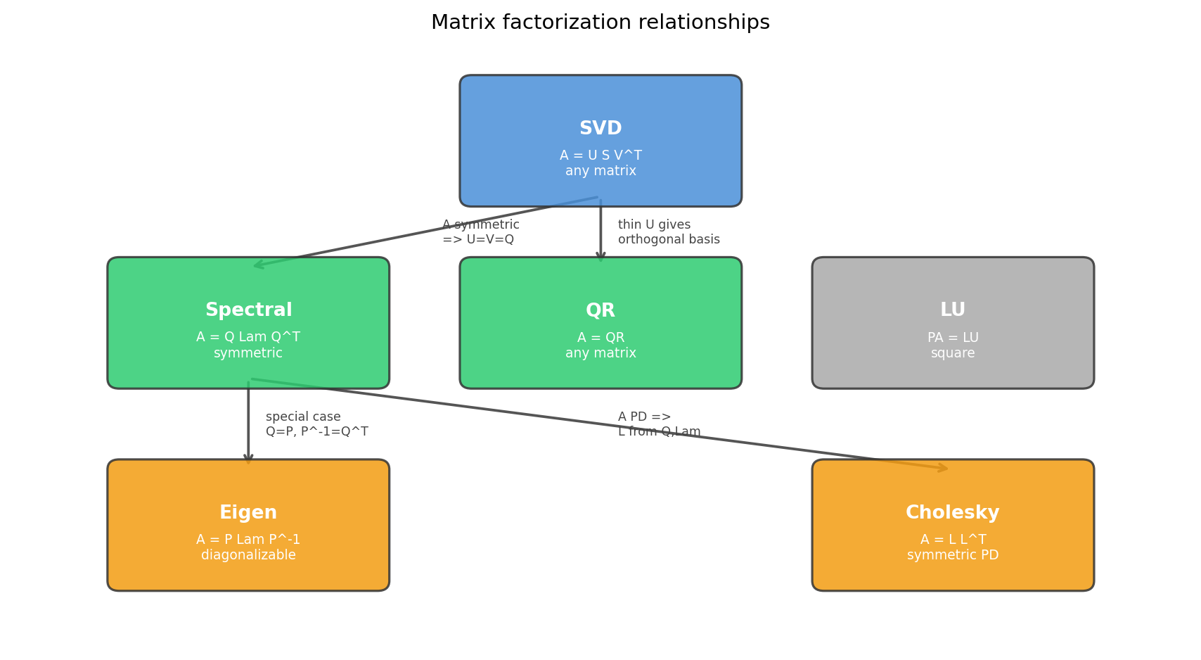
nodes = {
    'SVD':   (5.0, 5.0),
    'Spectral': (2.0, 3.2),
    'QR':    (5.0, 3.2),
    'LU':    (8.0, 3.2),
    'Eigen': (2.0, 1.2),
    'Cholesky': (8.0, 1.2),
}
colors = {
    'SVD': '#4a90d9',
    'Spectral': '#2ecc71',
    'QR': '#2ecc71',
    'LU': '#aaaaaa',
    'Eigen': '#f39c12',
    'Cholesky': '#f39c12',
}
descriptions = {
    'SVD':      'A = U S V^T\nany matrix',
    'Spectral': 'A = Q Lam Q^T\nsymmetric',
    'QR':       'A = QR\nany matrix',
    'LU':       'PA = LU\nsquare',
    'Eigen':    'A = P Lam P^-1\ndiagonalizable',
    'Cholesky': 'A = L L^T\nsymmetric PD',
}

for name, (x, y) in nodes.items():
    box = mpatches.FancyBboxPatch(
        (x - 1.1, y - 0.55), 2.2, 1.1,
        boxstyle='round,pad=0.1',
        facecolor=colors[name], edgecolor='#333333',
        linewidth=1.2, alpha=0.85, zorder=3,
    )
    ax.add_patch(box)
    ax.text(x, y + 0.12, name, ha='center', va='center',
            fontsize=10, fontweight='bold', color='white', zorder=4)
    ax.text(x, y - 0.22, descriptions[name], ha='center', va='center',
            fontsize=7, color='white', zorder=4)

edges = [
    ('SVD', 'Spectral', 'A symmetric\n=> U=V=Q'),
    ('SVD', 'QR',        'thin U gives\northogonal basis'),
    ('Spectral', 'Eigen', 'special case\nQ=P, P^-1=Q^T'),
    ('Spectral', 'Cholesky', 'A PD =>\nL from Q,Lam'),
]

for src, dst, label in edges:
    x0, y0 = nodes[src]
    x1, y1 = nodes[dst]
    ax.annotate('', xy=(x1, y1 + 0.55), xytext=(x0, y0 - 0.55),
                arrowprops=dict(arrowstyle='->', color='#555555', lw=1.4),
                zorder=2)
    mx, my = (x0 + x1) / 2, (y0 + y1) / 2
    ax.text(mx + 0.15, my, label, ha='left', va='center',
            fontsize=6.5, color='#444444', zorder=4)

ax.set_title('Matrix factorization relationships', fontsize=11)
plt.tight_layout()
plt.show()

Figure 27.2: Relationships among the six major factorizations. SVD is the most general and subsumes several others as special cases. Arrows indicate ‘can be derived from’ or ‘is a special case of’.

---

27.7.3 Conditioning and Numerical Stability at a Glance

import numpy as np
import scipy.linalg

rng = np.random.default_rng(0)
n = 6
A = rng.standard_normal((n, n))
A = A @ A.T + n * np.eye(n)     # shape (6, 6)  SPD

kappa = np.linalg.cond(A)

P_mat, L, U = scipy.linalg.lu(A)
Q, R = np.linalg.qr(A)
vals, _ = np.linalg.eigh(A)
U_s, s, Vt = np.linalg.svd(A, full_matrices=False)

print(f"Condition number kappa(A)      : {kappa:.2f}")
print(f"kappa via singular values       : {s[0]/s[-1]:.2f}")
print(f"kappa via eigenvalues (eigh)    : {vals[-1]/vals[0]:.2f}")
print(f"kappa via LU (U diagonal ratio) : {np.abs(np.diag(U)[0]/np.diag(U)[-1]):.2f}")

Condition number kappa(A)      : 2.67
kappa via singular values       : 2.67
kappa via eigenvalues (eigh)    : 2.67
kappa via LU (U diagonal ratio) : 1.01

All three estimates of condition number should agree for a well-formed SPD matrix. Large condition numbers (\(\kappa \gg 10^6\)) mean the system is nearly singular and solutions will have \(\log_{10}(\kappa)\) digits of accuracy lost.