4  Vectors in ℝⁿ

4.1 Vectors: Point, Displacement, Direction

The word “vector” means different things depending on context — and getting this wrong causes subtle bugs in 3D graphics and robotics. A 3-tuple \((x, y, z)\) can represent:

Interpretation Meaning Transforms under rotation \(R\) as
Point (position) A location in space \(R\mathbf{p} + \mathbf{t}\) (rotate and translate)
Displacement (free vector) A difference of two positions \(R\mathbf{d}\) (rotate only, translation cancels)
Direction (unit vector) A normalized displacement \(R\hat{\mathbf{u}}\) (same as displacement; \(\|\hat{\mathbf{u}}\|=1\) preserved)

Chapter 9 will make this precise with SE(3) and homogeneous coordinates. For now, the key habit: always know which interpretation you intend.


4.1.1 Points and Displacements in ℝⁿ

A point \(\mathbf{p} \in \mathbb{R}^n\) specifies a location relative to some origin. Its numerical values depend on where the origin is.

A displacement \(\mathbf{d} = \mathbf{q} - \mathbf{p}\) is the difference of two points. Displacements are free vectors — shifting the origin does not change \(\mathbf{d}\).

\[\mathbf{d} = \mathbf{q} - \mathbf{p} = \begin{pmatrix}q_1 - p_1 \\ q_2 - p_2 \\ \vdots \\ q_n - p_n\end{pmatrix}\]

import numpy as np

# Two 3D landmark positions (points)
p = np.array([1.0, 2.0, 0.5])   # robot at p
q = np.array([4.0, 3.0, 1.5])   # goal at q

# Displacement from p to q
d = q - p
print(f"Displacement d = q - p: {d}")
print(f"Euclidean distance:      {np.linalg.norm(d):.4f} m")

# Key: if we shift origin by t, points change but displacement does not
t = np.array([10.0, -5.0, 3.0])   # arbitrary origin shift
p_new = p + t
q_new = q + t
d_new = q_new - p_new
print(f"\nAfter shifting origin by {t}:")
print(f"  p_new = {p_new}, q_new = {q_new}")
print(f"  Displacement unchanged: {d_new}")
print(f"  Same as before: {np.allclose(d, d_new)}")
Displacement d = q - p: [3. 1. 1.]
Euclidean distance:      3.3166 m

After shifting origin by [10. -5.  3.]:
  p_new = [11.  -3.   3.5], q_new = [14.  -2.   4.5]
  Displacement unchanged: [3. 1. 1.]
  Same as before: True

4.1.2 Unit Vectors (Directions)

A direction is a displacement normalized to unit length:

\[\hat{\mathbf{u}} = \frac{\mathbf{d}}{\|\mathbf{d}\|}, \qquad \|\hat{\mathbf{u}}\| = 1\]

Directions appear in: - Surface normals (Ch 4.3, App) - Axis of rotation in Rodrigues’ formula (Ch 8) - Principal directions from SVD (Ch 18) - Camera viewing rays (Ch 10)

import numpy as np

d = np.array([3.0, -4.0, 0.0])
norm_d = np.linalg.norm(d)
u_hat = d / norm_d

print(f"d     = {d}")
print(f"‖d‖   = {norm_d:.4f}")
print(f"û     = {u_hat}")
print(f"‖û‖   = {np.linalg.norm(u_hat):.10f}  (should be 1.0)")
d     = [ 3. -4.  0.]
‖d‖   = 5.0000
û     = [ 0.6 -0.8  0. ]
‖û‖   = 1.0000000000  (should be 1.0)

Pitfall — zero-length vectors. Normalizing a zero vector produces nan. Always guard in production code:

def safe_normalize(v, tol=1e-12):
    """Return unit vector, or zero if v is too short."""
    n = np.linalg.norm(v)
    return v / n if n > tol else np.zeros_like(v)

4.1.3 Standard Basis Vectors

The standard basis of \(\mathbb{R}^n\) consists of unit vectors along each axis:

\[\mathbf{e}_1 = \begin{pmatrix}1\\0\\\vdots\\0\end{pmatrix}, \quad \mathbf{e}_2 = \begin{pmatrix}0\\1\\\vdots\\0\end{pmatrix}, \quad \ldots, \quad \mathbf{e}_n = \begin{pmatrix}0\\\vdots\\0\\1\end{pmatrix}\]

Any vector \(\mathbf{v} \in \mathbb{R}^n\) decomposes as:

\[\mathbf{v} = v_1\mathbf{e}_1 + v_2\mathbf{e}_2 + \cdots + v_n\mathbf{e}_n\]

The components \(v_i\) are the coordinates of \(\mathbf{v}\) in the standard basis. Section 4.5 generalizes this to arbitrary bases.

import numpy as np

n = 4
E = np.eye(n)   # columns are e_1, ..., e_n

v = np.array([2.0, -1.0, 3.0, 0.5])
print("Standard basis vectors (columns of I_4):")
for i in range(n):
    print(f"  e_{i+1} = {E[:, i]}")

# Reconstruct v from its components
v_reconstructed = sum(v[i] * E[:, i] for i in range(n))
print(f"\nv = {v}")
print(f"Reconstructed: {v_reconstructed}")
print(f"Match: {np.allclose(v, v_reconstructed)}")
Standard basis vectors (columns of I_4):
  e_1 = [1. 0. 0. 0.]
  e_2 = [0. 1. 0. 0.]
  e_3 = [0. 0. 1. 0.]
  e_4 = [0. 0. 0. 1.]

v = [ 2.  -1.   3.   0.5]
Reconstructed: [ 2.  -1.   3.   0.5]
Match: True

4.1.4 Visualizing Vectors: Points vs. Displacements

import numpy as np
import matplotlib.pyplot as plt

fig, axes = plt.subplots(1, 3, figsize=(12, 4))
titles = ['Point\n(absolute position)', 'Displacement\n(free vector)',
          'Direction\n(unit vector)']

origin = np.array([0, 0])
P = np.array([2.5, 1.5])
Q = np.array([0.5, 3.0])
blue  = '#4a90d9'
green = '#2ecc71'
red   = 'tomato'

# --- Panel 1: Points ---
ax = axes[0]
ax.annotate('', xy=P, xytext=origin,
            arrowprops=dict(arrowstyle='->', color=blue, lw=2))
ax.annotate('', xy=Q, xytext=origin,
            arrowprops=dict(arrowstyle='->', color=green, lw=2))
ax.scatter(*origin, color='#333333', s=60, zorder=5)
ax.text(*P + 0.1, 'p', color=blue, fontsize=13, fontweight='bold')
ax.text(*Q + 0.1, 'q', color=green, fontsize=13, fontweight='bold')
ax.text(0.1, -0.3, 'O (origin)', color='#333333', fontsize=9)

# --- Panel 2: Displacement ---
ax = axes[1]
ax.annotate('', xy=P, xytext=origin,
            arrowprops=dict(arrowstyle='->', color=blue, lw=1.5,
                            linestyle='dashed', alpha=0.4))
ax.annotate('', xy=Q, xytext=origin,
            arrowprops=dict(arrowstyle='->', color=green, lw=1.5,
                            linestyle='dashed', alpha=0.4))
ax.annotate('', xy=Q, xytext=P,
            arrowprops=dict(arrowstyle='->', color=red, lw=2.5))
ax.text(*(P + Q) / 2 + np.array([0.15, 0.0]),
        'd = q − p', color=red, fontsize=11, fontweight='bold')
ax.scatter(*origin, color='#333333', s=50, zorder=5)

p2 = np.array([1.2, 0.2])
q2 = p2 + (Q - P)
ax.annotate('', xy=q2, xytext=p2,
            arrowprops=dict(arrowstyle='->', color=red, lw=2.5, alpha=0.4))
ax.text(*(p2 + q2) / 2 + np.array([0.1, 0.1]),
        'd (shifted)', color=red, fontsize=9, alpha=0.6)

# --- Panel 3: Direction ---
ax = axes[2]
d = Q - P
d_hat = d / np.linalg.norm(d)
ax.annotate('', xy=P + d, xytext=P,
            arrowprops=dict(arrowstyle='->', color=red, lw=1.5,
                            linestyle='dashed', alpha=0.4))
ax.annotate('', xy=P + d_hat, xytext=P,
            arrowprops=dict(arrowstyle='->', color=green, lw=2.5))
ax.text(*(P + d_hat) + np.array([0.1, 0.0]),
        'û  (‖û‖=1)', color=green, fontsize=11, fontweight='bold')
ax.text(*(P + d) + np.array([0.1, 0.0]),
        'd', color=red, fontsize=11, alpha=0.5)

for ax, title in zip(axes, titles):
    ax.set_xlim(-0.5, 4.0); ax.set_ylim(-0.5, 4.0)
    ax.set_aspect('equal')
    ax.set_title(title, fontsize=11, pad=8)
    ax.tick_params(labelsize=8)

fig.suptitle('Three interpretations of a vector', fontsize=13, y=1.01)
fig.tight_layout()
plt.show()


4.1.5 Why the Distinction Matters in Robotics

Consider a robot arm with a tool attached. When the arm rotates by \(R\):

  • The tool position (a point) transforms as \(R\mathbf{p} + \mathbf{t}\) — it both rotates and translates relative to the base.
  • The tool orientation direction (e.g., the \(z\)-axis of the tool frame) transforms as \(R\hat{\mathbf{z}}\) — rotation only, no translation.
  • A force applied at the tool tip is a free vector: it transforms as \(R\mathbf{f}\), unaffected by where the tool is.

Homogeneous coordinates (Ch 7) unify all three in a single 4×4 matrix by encoding the distinction in the last component:

\[\text{point:} \begin{pmatrix}\mathbf{p} \\ 1\end{pmatrix}, \qquad \text{direction:} \begin{pmatrix}\hat{\mathbf{u}} \\ 0\end{pmatrix}\]

The 1 vs. 0 in the last slot is what causes the translation to apply (or not) when you multiply by the 4×4 homogeneous matrix.

import numpy as np

# 2D example with homogeneous coordinates
# Rotation by 90°, translation by [3, 1]
theta = np.pi / 2
R2 = np.array([[np.cos(theta), -np.sin(theta)],
               [np.sin(theta),  np.cos(theta)]])
t = np.array([3.0, 1.0])

T_hom = np.eye(3)
T_hom[:2, :2] = R2
T_hom[:2, 2]  = t

p_h = np.array([1.0, 0.0, 1.0])   # point at (1,0), last component = 1
d_h = np.array([1.0, 0.0, 0.0])   # direction along x, last component = 0

p_transformed = T_hom @ p_h
d_transformed = T_hom @ d_h

print(f"Homogeneous transform T:\n{T_hom}")
print(f"\nPoint (1,0):   {p_h[:2]}{p_transformed[:2]}")
print(f"  (rotated AND translated)")
print(f"\nDirection (1,0): {d_h[:2]}{d_transformed[:2]}")
print(f"  (rotated only — last 0 blocks translation)")
Homogeneous transform T:
[[ 6.123234e-17 -1.000000e+00  3.000000e+00]
 [ 1.000000e+00  6.123234e-17  1.000000e+00]
 [ 0.000000e+00  0.000000e+00  1.000000e+00]]

Point (1,0):   [1. 0.] → [3. 2.]
  (rotated AND translated)

Direction (1,0): [1. 0.] → [6.123234e-17 1.000000e+00]
  (rotated only — last 0 blocks translation)

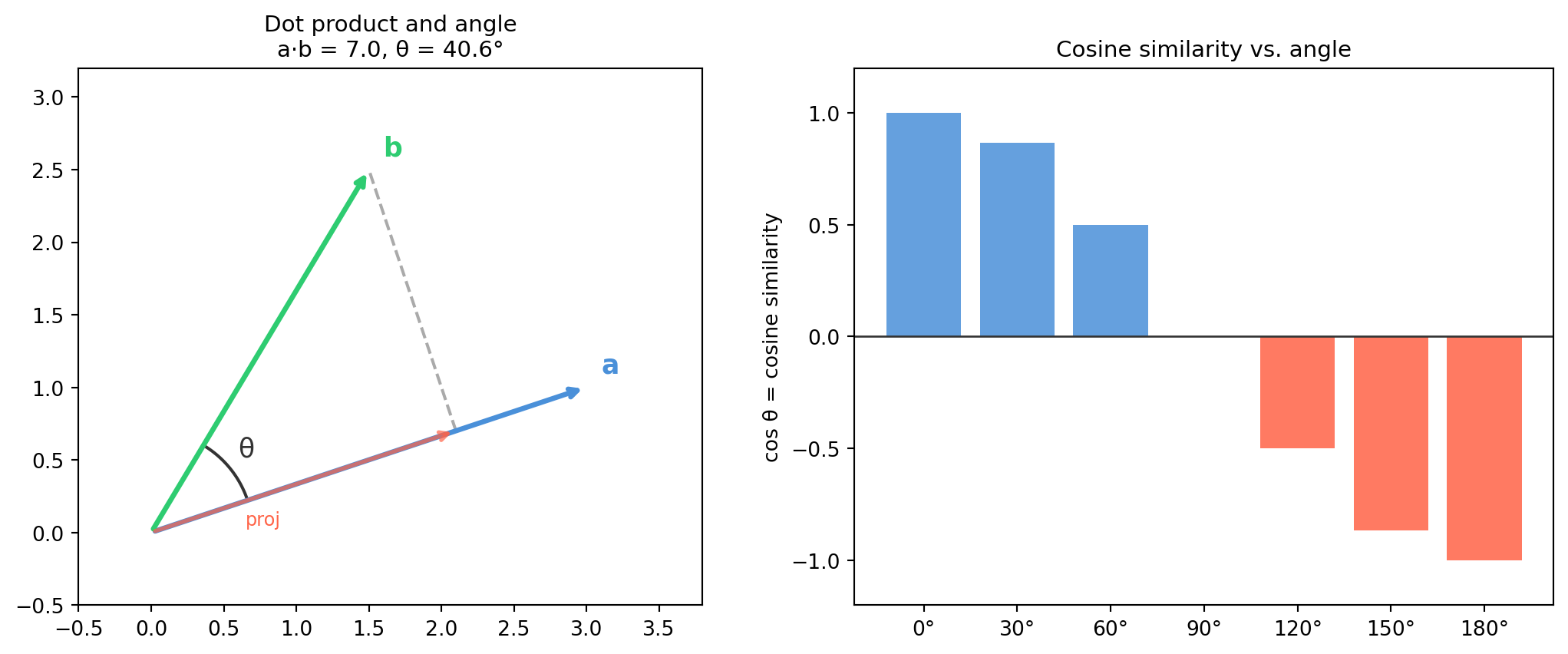
4.2 Dot Product, Angle, and Cosine Similarity

The dot product is the workhorse of inner products. It computes in \(O(n)\) time and underlies projection, similarity search, neural network layers, and the definition of angles in any dimension.


4.2.1 Definition and Geometric Meaning

For \(\mathbf{a}, \mathbf{b} \in \mathbb{R}^n\):

\[\mathbf{a} \cdot \mathbf{b} = \sum_{i=1}^{n} a_i b_i = \mathbf{a}^T\mathbf{b}\]

Geometric identity:

\[\mathbf{a} \cdot \mathbf{b} = \|\mathbf{a}\|\,\|\mathbf{b}\|\cos\theta\]

where \(\theta \in [0, \pi]\) is the angle between the vectors. Rearranging:

\[\cos\theta = \frac{\mathbf{a} \cdot \mathbf{b}}{\|\mathbf{a}\|\,\|\mathbf{b}\|}\]

Sign of \(\mathbf{a}\cdot\mathbf{b}\) \(\theta\) Geometric meaning
\(> 0\) \(< 90°\) Same general direction
\(= 0\) \(= 90°\) Orthogonal (perpendicular)
\(< 0\) \(> 90°\) Opposing directions
import numpy as np

a = np.array([3.0, 1.0, 0.0])
b = np.array([1.0, 2.0, 0.0])

dot = np.dot(a, b)              # same as a @ b
cos_theta = dot / (np.linalg.norm(a) * np.linalg.norm(b))
theta_deg = np.degrees(np.arccos(np.clip(cos_theta, -1.0, 1.0)))

print(f"a · b     = {dot:.4f}")
print(f"cos θ     = {cos_theta:.4f}")
print(f"θ         = {theta_deg:.2f}°")

# Verify with three cases
pairs = [
    (np.array([1., 0.]), np.array([1., 0.])),    # same direction
    (np.array([1., 0.]), np.array([0., 1.])),    # perpendicular
    (np.array([1., 0.]), np.array([-1., 0.])),   # opposite
]
for u, v in pairs:
    c = np.dot(u, v) / (np.linalg.norm(u) * np.linalg.norm(v))
    print(f"  {u} · {v} → cos θ = {c:.1f}, θ = {np.degrees(np.arccos(c)):.0f}°")
a · b     = 5.0000
cos θ     = 0.7071
θ         = 45.00°
  [1. 0.] · [1. 0.] → cos θ = 1.0, θ = 0°
  [1. 0.] · [0. 1.] → cos θ = 0.0, θ = 90°
  [1. 0.] · [-1.  0.] → cos θ = -1.0, θ = 180°

4.2.2 Properties of the Dot Product

The dot product satisfies:

  1. Symmetry: \(\mathbf{a}\cdot\mathbf{b} = \mathbf{b}\cdot\mathbf{a}\)
  2. Linearity: \(\mathbf{a}\cdot(c\mathbf{b}+\mathbf{d}) = c(\mathbf{a}\cdot\mathbf{b}) + \mathbf{a}\cdot\mathbf{d}\)
  3. Positive-definiteness: \(\mathbf{a}\cdot\mathbf{a} \geq 0\), with equality iff \(\mathbf{a} = \mathbf{0}\)
  4. Self-dot = squared norm: \(\mathbf{a}\cdot\mathbf{a} = \|\mathbf{a}\|^2\)

Property 4 gives an efficient norm computation: np.dot(a, a) skips the square root.

import numpy as np

a = np.array([3.0, 4.0])
print(f"a · a = {np.dot(a, a)}")
print(f"‖a‖²  = {np.linalg.norm(a)**2}")
print(f"‖a‖   = {np.sqrt(np.dot(a, a)):.4f}  (Pythagorean: sqrt(9+16) = 5)")
a · a = 25.0
‖a‖²  = 25.0
‖a‖   = 5.0000  (Pythagorean: sqrt(9+16) = 5)

4.2.3 Projection via the Dot Product

The scalar projection of \(\mathbf{b}\) onto direction \(\hat{\mathbf{a}}\):

\[\text{proj}_{\hat{\mathbf{a}}} \mathbf{b} = \mathbf{b} \cdot \hat{\mathbf{a}}\]

The vector projection (the component of \(\mathbf{b}\) along \(\mathbf{a}\)):

\[\text{proj}_{\mathbf{a}} \mathbf{b} = \frac{\mathbf{a}\cdot\mathbf{b}}{\mathbf{a}\cdot\mathbf{a}}\,\mathbf{a}\]

The rejection (perpendicular component):

\[\text{rej}_{\mathbf{a}} \mathbf{b} = \mathbf{b} - \text{proj}_{\mathbf{a}} \mathbf{b}\]

This decomposition is the basis of Gram-Schmidt orthogonalization (Ch 16) and least-squares projection (Ch 17).

import numpy as np

a = np.array([3.0, 0.0])    # project onto x-axis direction
b = np.array([2.0, 2.5])

proj = (np.dot(a, b) / np.dot(a, a)) * a
rej  = b - proj

print(f"b         = {b}")
print(f"proj_a(b) = {proj}   (component along a)")
print(f"rej_a(b)  = {rej}    (perpendicular component)")
print(f"Reconstruction check: proj + rej = {proj + rej}")
print(f"Orthogonality check: proj · rej = {np.dot(proj, rej):.10f}")
b         = [2.  2.5]
proj_a(b) = [2. 0.]   (component along a)
rej_a(b)  = [0.  2.5]    (perpendicular component)
Reconstruction check: proj + rej = [2.  2.5]
Orthogonality check: proj · rej = 0.0000000000

4.2.4 Cosine Similarity

The cosine similarity removes magnitude, keeping only direction:

\[\text{sim}(\mathbf{a}, \mathbf{b}) = \frac{\mathbf{a}\cdot\mathbf{b}}{\|\mathbf{a}\|\,\|\mathbf{b}\|} \in [-1, 1]\]

It is the inner product of the unit vectors \(\hat{\mathbf{a}}\) and \(\hat{\mathbf{b}}\).

When to use cosine similarity vs. Euclidean distance:

Use case Preferred metric Reason
Embedding retrieval (CLIP, BERT) Cosine Scale invariant; magnitudes differ across contexts
k-NN in pixel space Euclidean Magnitude carries meaningful information
Feature matching (ORB, SIFT) Dot product on normalized descriptors Cosine but precomputed normalization
Anomaly detection Mahalanobis Accounts for feature correlations
import numpy as np

def cosine_similarity(a, b):
    """Cosine similarity between two vectors."""
    return np.dot(a, b) / (np.linalg.norm(a) * np.linalg.norm(b))

# Word embedding analogy: "king" and "queen" vs. "king" and "bicycle"
# (using toy 4-D embeddings)
king   = np.array([0.9,  0.4, -0.1,  0.5])
queen  = np.array([0.85, 0.3,  0.2,  0.6])
bicycle= np.array([-0.2, 0.1,  0.9, -0.3])

print(f"sim(king, queen)   = {cosine_similarity(king, queen):.4f}  (high)")
print(f"sim(king, bicycle) = {cosine_similarity(king, bicycle):.4f}  (low)")

# Batch cosine similarity: normalize first, then use matrix multiply
embeddings = np.vstack([king, queen, bicycle])
norms = np.linalg.norm(embeddings, axis=1, keepdims=True)
embeddings_n = embeddings / norms

sim_matrix = embeddings_n @ embeddings_n.T
labels = ['king', 'queen', 'bicycle']
print("\nSimilarity matrix:")
for i, row_label in enumerate(labels):
    for j, col_label in enumerate(labels):
        print(f"  sim({row_label:7s}, {col_label:7s}) = {sim_matrix[i,j]:.4f}")
sim(king, queen)   = 0.9540  (high)
sim(king, bicycle) = -0.3515  (low)

Similarity matrix:
  sim(king   , king   ) = 1.0000
  sim(king   , queen  ) = 0.9540
  sim(king   , bicycle) = -0.3515
  sim(queen  , king   ) = 0.9540
  sim(queen  , queen  ) = 1.0000
  sim(queen  , bicycle) = -0.1304
  sim(bicycle, king   ) = -0.3515
  sim(bicycle, queen  ) = -0.1304
  sim(bicycle, bicycle) = 1.0000

4.2.5 Batch Dot Products: Matrix Form

If you have \(m\) query vectors (rows of \(Q \in \mathbb{R}^{m\times n}\)) and \(k\) database vectors (rows of \(D \in \mathbb{R}^{k\times n}\)), all pairwise dot products are:

\[S = Q D^T \in \mathbb{R}^{m \times k}\]

This is the central computation in approximate nearest-neighbor search, attention mechanisms in transformers, and feature correlation in CV.

import numpy as np

# 3 queries, 5 database vectors, 4-dimensional embeddings
rng = np.random.default_rng(0)
Q = rng.standard_normal((3, 4))
D = rng.standard_normal((5, 4))

# Normalize for cosine similarity
Q_n = Q / np.linalg.norm(Q, axis=1, keepdims=True)
D_n = D / np.linalg.norm(D, axis=1, keepdims=True)

S = Q_n @ D_n.T   # shape (3, 5)
print(f"Similarity matrix shape: {S.shape}")
print("Nearest neighbor for each query (index of max similarity):")
for i in range(3):
    best = np.argmax(S[i])
    print(f"  Query {i}: best match is DB[{best}], sim = {S[i, best]:.4f}")
Similarity matrix shape: (3, 5)
Nearest neighbor for each query (index of max similarity):
  Query 0: best match is DB[1], sim = 0.3997
  Query 1: best match is DB[1], sim = 0.7622
  Query 2: best match is DB[0], sim = 0.6141

4.2.6 Visualizing the Dot Product

import numpy as np
import matplotlib.pyplot as plt

fig, axes = plt.subplots(1, 2, figsize=(11, 4.5))

# --- Panel 1: Angle visualization ---
ax = axes[0]
origin = np.zeros(2)
a = np.array([3.0, 1.0])
b = np.array([1.5, 2.5])

ax.annotate('', xy=a, xytext=origin,
            arrowprops=dict(arrowstyle='->', color='#4a90d9', lw=2.5))
ax.annotate('', xy=b, xytext=origin,
            arrowprops=dict(arrowstyle='->', color='#2ecc71', lw=2.5))

proj = (np.dot(a, b) / np.dot(a, a)) * a
ax.annotate('', xy=proj, xytext=origin,
            arrowprops=dict(arrowstyle='->', color='tomato', lw=2, alpha=0.7))
ax.plot([proj[0], b[0]], [proj[1], b[1]], '--', color='#aaaaaa', lw=1.5)

theta_a = np.arctan2(a[1], a[0])
theta_b = np.arctan2(b[1], b[0])
arc_r = 0.7
thetas = np.linspace(theta_a, theta_b, 60)
ax.plot(arc_r * np.cos(thetas), arc_r * np.sin(thetas), color='#333333', lw=1.5)
mid = (theta_a + theta_b) / 2
ax.text(arc_r * 1.2 * np.cos(mid), arc_r * 1.2 * np.sin(mid), 'θ',
        color='#333333', fontsize=13, ha='center')

cos_theta = np.dot(a, b) / (np.linalg.norm(a) * np.linalg.norm(b))
theta_deg = np.degrees(np.arccos(cos_theta))
ax.set_title(f'Dot product and angle\na·b = {np.dot(a,b):.1f}, θ = {theta_deg:.1f}°', fontsize=11)
ax.text(*a + 0.1, 'a', color='#4a90d9', fontsize=13, fontweight='bold')
ax.text(*b + 0.1, 'b', color='#2ecc71', fontsize=13, fontweight='bold')
ax.text(*proj / 2 + np.array([-0.4, -0.3]), 'proj', color='tomato', fontsize=9)
ax.set_xlim(-0.5, 3.8); ax.set_ylim(-0.5, 3.2)
ax.set_aspect('equal')

# --- Panel 2: Cosine similarity bar chart ---
ax = axes[1]
angles = [0, 30, 60, 90, 120, 150, 180]
sims = [np.cos(np.radians(a)) for a in angles]
colors_bar = ['#4a90d9' if s > 0 else ('#aaaaaa' if abs(s) < 1e-9 else 'tomato') for s in sims]
ax.bar([f'{a}°' for a in angles], sims, color=colors_bar, alpha=0.85)
ax.axhline(0, color='#333333', lw=1)
ax.set_ylim(-1.2, 1.2)
ax.set_ylabel('cos θ = cosine similarity')
ax.set_title('Cosine similarity vs. angle', fontsize=11)

fig.tight_layout()
plt.show()


4.2.7 Cauchy-Schwarz Inequality

\[|\mathbf{a} \cdot \mathbf{b}| \leq \|\mathbf{a}\|\,\|\mathbf{b}\|\]

Equality holds if and only if \(\mathbf{a}\) and \(\mathbf{b}\) are parallel (one is a scalar multiple of the other). This is what guarantees \(\cos\theta\) is always in \([-1, 1]\) — the inequality says the dot product can never exceed the product of the norms.

import numpy as np

rng = np.random.default_rng(42)
n = 100

# Test Cauchy-Schwarz on random vectors
for _ in range(5):
    a = rng.standard_normal(n)
    b = rng.standard_normal(n)
    lhs = abs(np.dot(a, b))
    rhs = np.linalg.norm(a) * np.linalg.norm(b)
    print(f"|a·b| = {lhs:.4f} ≤ ‖a‖‖b‖ = {rhs:.4f}{lhs <= rhs + 1e-12}")
|a·b| = 7.1705 ≤ ‖a‖‖b‖ = 75.4795  ✓ True
|a·b| = 4.4166 ≤ ‖a‖‖b‖ = 103.4563  ✓ True
|a·b| = 6.9440 ≤ ‖a‖‖b‖ = 103.1418  ✓ True
|a·b| = 9.8055 ≤ ‖a‖‖b‖ = 102.9934  ✓ True
|a·b| = 2.8561 ≤ ‖a‖‖b‖ = 101.7937  ✓ True

4.3 Cross Product and Surface Normals

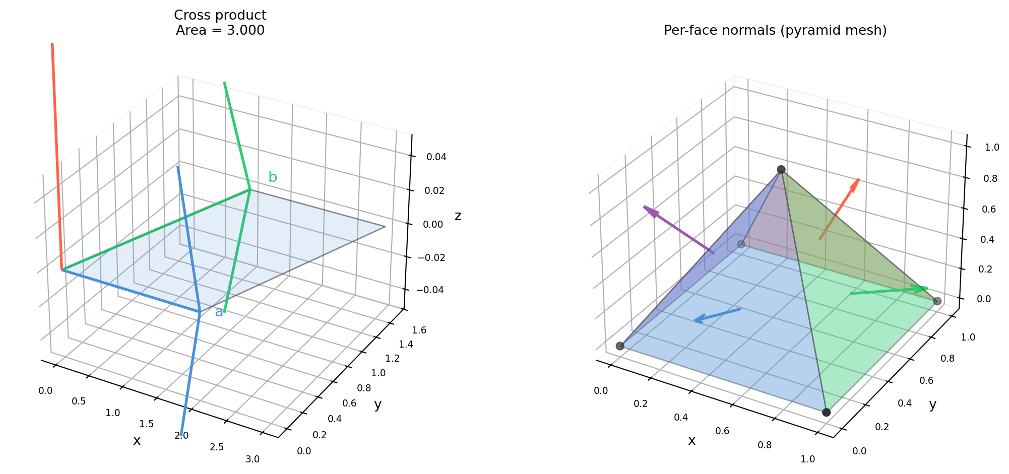
The cross product is unique to \(\mathbb{R}^3\) (and, in a generalized sense, \(\mathbb{R}^7\)). It produces a vector perpendicular to both inputs, with magnitude equal to the area of the parallelogram they span. In robotics and computer vision it appears everywhere: surface normals, torque, angular velocity, and the essential matrix in epipolar geometry.


4.3.1 Definition

For \(\mathbf{a}, \mathbf{b} \in \mathbb{R}^3\):

\[\mathbf{a} \times \mathbf{b} = \begin{vmatrix}\mathbf{e}_1 & \mathbf{e}_2 & \mathbf{e}_3 \\ a_1 & a_2 & a_3 \\ b_1 & b_2 & b_3\end{vmatrix} = \begin{pmatrix} a_2 b_3 - a_3 b_2 \\ a_3 b_1 - a_1 b_3 \\ a_1 b_2 - a_2 b_1 \end{pmatrix}\]

Key properties:

Property Formula Physical meaning
Anti-symmetry \(\mathbf{a}\times\mathbf{b} = -\mathbf{b}\times\mathbf{a}\) Order determines sign of normal
Magnitude \(\|\mathbf{a}\times\mathbf{b}\| = \|\mathbf{a}\|\|\mathbf{b}\|\sin\theta\) Area of parallelogram
Orthogonality \((\mathbf{a}\times\mathbf{b})\cdot\mathbf{a} = 0\) Normal to both inputs
Parallel → zero \(\mathbf{a}\times\mathbf{a} = \mathbf{0}\) \(\sin 0 = 0\)
import numpy as np

a = np.array([1.0, 0.0, 0.0])   # x-axis
b = np.array([0.0, 1.0, 0.0])   # y-axis

c = np.cross(a, b)   # should be z-axis = [0, 0, 1]
print(f"a × b = {c}   (right-hand rule: x × y = z)")
print(f"b × a = {np.cross(b, a)}   (anti-symmetry: y × x = -z)")
print(f"‖a × b‖ = {np.linalg.norm(c):.4f}  (= area of unit square)")

# General case
a2 = np.array([2.0, 1.0, 0.0])
b2 = np.array([1.0, 2.0, 0.0])
c2 = np.cross(a2, b2)
area = np.linalg.norm(c2)
theta = np.arcsin(area / (np.linalg.norm(a2) * np.linalg.norm(b2)))
print(f"\na2 = {a2}, b2 = {b2}")
print(f"a2 × b2 = {c2}")
print(f"Parallelogram area = {area:.4f}")
print(f"θ = {np.degrees(theta):.2f}°")

# Verify orthogonality
print(f"\nOrthogonality checks:")
print(f"  (a2 × b2) · a2 = {np.dot(c2, a2):.10f}")
print(f"  (a2 × b2) · b2 = {np.dot(c2, b2):.10f}")
a × b = [0. 0. 1.]   (right-hand rule: x × y = z)
b × a = [ 0.  0. -1.]   (anti-symmetry: y × x = -z)
‖a × b‖ = 1.0000  (= area of unit square)

a2 = [2. 1. 0.], b2 = [1. 2. 0.]
a2 × b2 = [0. 0. 3.]
Parallelogram area = 3.0000
θ = 36.87°

Orthogonality checks:
  (a2 × b2) · a2 = 0.0000000000
  (a2 × b2) · b2 = 0.0000000000

4.3.2 Right-Hand Rule

The direction of \(\mathbf{a} \times \mathbf{b}\) follows the right-hand rule: curl the fingers of your right hand from \(\mathbf{a}\) toward \(\mathbf{b}\); the thumb points in the direction of the cross product.

Standard basis cross products:

\[\mathbf{e}_1 \times \mathbf{e}_2 = \mathbf{e}_3, \quad \mathbf{e}_2 \times \mathbf{e}_3 = \mathbf{e}_1, \quad \mathbf{e}_3 \times \mathbf{e}_1 = \mathbf{e}_2\]

(Cyclic: \(1\to2\to3\to1\); reversing any pair negates the result.)


4.3.3 Skew-Symmetric Matrix Form

The cross product \(\mathbf{a} \times \mathbf{b}\) is linear in \(\mathbf{b}\), so it can be written as matrix multiplication. Define the skew-symmetric (or “hat”) matrix of \(\mathbf{a}\):

\[[\mathbf{a}]_\times = \begin{pmatrix} 0 & -a_3 & a_2 \\ a_3 & 0 & -a_1 \\ -a_2 & a_1 & 0 \end{pmatrix}\]

Then \(\mathbf{a} \times \mathbf{b} = [\mathbf{a}]_\times \mathbf{b}\).

This matrix form is essential in: - Angular velocity: \(\dot{R} = [\boldsymbol{\omega}]_\times R\) - Rodrigues’ rotation formula (Ch 8) - Essential matrix in epipolar geometry (Ch 25)

import numpy as np

def skew(a):
    """Skew-symmetric matrix [a]× such that [a]× b = a × b."""
    return np.array([[ 0,    -a[2],  a[1]],
                     [ a[2],  0,    -a[0]],
                     [-a[1],  a[0],  0   ]])

a = np.array([1.0, 2.0, 3.0])
b = np.array([4.0, 5.0, 6.0])

cross_direct = np.cross(a, b)
cross_matrix = skew(a) @ b

print(f"a × b (np.cross):     {cross_direct}")
print(f"[a]× @ b (matrix):    {cross_matrix}")
print(f"Match: {np.allclose(cross_direct, cross_matrix)}")

# Verify skew-symmetric: A^T = -A
A = skew(a)
print(f"\nSkew-symmetric check: A + A^T = \n{(A + A.T).round(10)}")
a × b (np.cross):     [-3.  6. -3.]
[a]× @ b (matrix):    [-3.  6. -3.]
Match: True

Skew-symmetric check: A + A^T = 
[[0. 0. 0.]
 [0. 0. 0.]
 [0. 0. 0.]]

4.3.4 Computing Surface Normals from Triangles

Given a triangle with vertices \(\mathbf{v}_0, \mathbf{v}_1, \mathbf{v}_2\):

\[\mathbf{n} = (\mathbf{v}_1 - \mathbf{v}_0) \times (\mathbf{v}_2 - \mathbf{v}_0)\]

The magnitude \(\|\mathbf{n}\|\) equals the triangle area; \(\hat{\mathbf{n}} = \mathbf{n}/\|\mathbf{n}\|\) is the unit normal.

import numpy as np

def triangle_normal(v0, v1, v2, normalize=True):
    """
    Compute the outward normal of a triangle.
    Vertex order (CCW when viewed from outside) follows right-hand rule.
    Returns (normal, area).
    """
    e1 = v1 - v0
    e2 = v2 - v0
    n  = np.cross(e1, e2)
    area = np.linalg.norm(n) / 2.0
    if normalize:
        n = n / np.linalg.norm(n)
    return n, area

# Unit square in the xy-plane (z=0), CCW from above
v0 = np.array([0.0, 0.0, 0.0])
v1 = np.array([1.0, 0.0, 0.0])
v2 = np.array([0.0, 1.0, 0.0])

n, area = triangle_normal(v0, v1, v2)
print(f"Triangle vertices: {v0}, {v1}, {v2}")
print(f"Normal:  {n}   (pointing in +z, as expected)")
print(f"Area:    {area:.4f} m²  (half of 1×1 square)")

# Tilted triangle
v0t = np.array([0., 0., 0.])
v1t = np.array([2., 0., 0.])
v2t = np.array([0., 2., 1.])
n_tilt, area_tilt = triangle_normal(v0t, v1t, v2t)
print(f"\nTilted triangle normal: {n_tilt.round(4)}")
print(f"Tilt area:              {area_tilt:.4f} m²")
Triangle vertices: [0. 0. 0.], [1. 0. 0.], [0. 1. 0.]
Normal:  [0. 0. 1.]   (pointing in +z, as expected)
Area:    0.5000 m²  (half of 1×1 square)

Tilted triangle normal: [ 0.     -0.4472  0.8944]
Tilt area:              2.2361 m²

4.3.5 Mesh Face Normals

Real meshes have thousands of triangles. Vectorized computation is critical.

import numpy as np

def mesh_face_normals(vertices, faces):
    """
    Compute per-face normals for a triangle mesh.
    vertices: (V, 3) array of vertex positions
    faces:    (F, 3) array of vertex indices
    Returns:  (F, 3) unit normals, (F,) face areas
    """
    v0 = vertices[faces[:, 0]]
    v1 = vertices[faces[:, 1]]
    v2 = vertices[faces[:, 2]]

    e1 = v1 - v0           # (F, 3)
    e2 = v2 - v0           # (F, 3)
    normals = np.cross(e1, e2)   # (F, 3)

    magnitudes = np.linalg.norm(normals, axis=1, keepdims=True)  # (F, 1)
    areas = magnitudes.flatten() / 2.0
    unit_normals = normals / np.maximum(magnitudes, 1e-12)       # avoid /0

    return unit_normals, areas

# Toy mesh: a box-like structure (4 triangles of a simple surface)
vertices = np.array([
    [0., 0., 0.],
    [1., 0., 0.],
    [1., 1., 0.],
    [0., 1., 0.],
    [0.5, 0.5, 1.],    # apex
], dtype=float)

faces = np.array([
    [0, 1, 4],
    [1, 2, 4],
    [2, 3, 4],
    [3, 0, 4],
], dtype=int)

normals, areas = mesh_face_normals(vertices, faces)
print(f"Face normals (shape {normals.shape}):")
for i, (n, a) in enumerate(zip(normals, areas)):
    print(f"  Face {i}: normal = {n.round(4)},  area = {a:.4f}")
Face normals (shape (4, 3)):
  Face 0: normal = [ 0.     -0.8944  0.4472],  area = 0.5590
  Face 1: normal = [ 0.8944 -0.      0.4472],  area = 0.5590
  Face 2: normal = [0.     0.8944 0.4472],  area = 0.5590
  Face 3: normal = [-0.8944  0.      0.4472],  area = 0.5590

4.3.6 Visualizing Cross Products and Normals

import numpy as np
import matplotlib.pyplot as plt
from mpl_toolkits.mplot3d import Axes3D
from mpl_toolkits.mplot3d.art3d import Poly3DCollection

fig = plt.figure(figsize=(12, 5))

# --- Left: cross product visualization ---
ax1 = fig.add_subplot(121, projection='3d')

a = np.array([2., 0., 0.])
b = np.array([1., 1.5, 0.])
c = np.cross(a, b)
c_hat = c / np.linalg.norm(c)

origin = np.zeros(3)
for vec, col, lbl in [(a, '#4a90d9', 'a'), (b, '#2ecc71', 'b'),
                       (c_hat * 1.5, 'tomato', 'a×b (unit)')]:
    ax1.quiver(*origin, *vec, color=col, arrow_length_ratio=0.15, lw=2)
    ax1.text(*(origin + vec * 1.1), lbl, color=col, fontsize=11)

corners = np.array([origin, a, a + b, b, origin])
ax1.plot(corners[:, 0], corners[:, 1], corners[:, 2],
         '-', color='#333333', lw=1, alpha=0.5)
poly = [[origin, a, a + b, b]]
col3d = Poly3DCollection(poly, alpha=0.15, facecolor='#4a90d9', edgecolor='#333333')
ax1.add_collection3d(col3d)
area = np.linalg.norm(c)
ax1.set_title(f'Cross product\nArea = {area:.3f}', fontsize=10)

# --- Right: face normals on a mesh ---
ax2 = fig.add_subplot(122, projection='3d')

vertices = np.array([[0,0,0],[1,0,0],[1,1,0],[0,1,0],[0.5,0.5,1.]], float)
faces = np.array([[0,1,4],[1,2,4],[2,3,4],[3,0,4]])

normals_mesh, areas_mesh = mesh_face_normals(vertices, faces)
colors_face = ['#4a90d9', '#2ecc71', 'tomato', '#9b59b6']

for face, n, a_f, col in zip(faces, normals_mesh, areas_mesh, colors_face):
    tri = vertices[face]
    poly = Poly3DCollection([tri], alpha=0.4, facecolor=col, edgecolor='#333333')
    ax2.add_collection3d(poly)
    centroid = tri.mean(axis=0)
    ax2.quiver(*centroid, *(n * 0.4),
               color=col, arrow_length_ratio=0.2, lw=2)

ax2.scatter(*vertices.T, color='#333333', s=30, zorder=5)
ax2.set_title('Per-face normals (pyramid mesh)', fontsize=10)

for ax in [ax1, ax2]:
    ax.set_xlabel('x', labelpad=2)
    ax.set_ylabel('y', labelpad=2)
    ax.set_zlabel('z', labelpad=2)
    ax.tick_params(labelsize=7)
    ax.xaxis.pane.fill = ax.yaxis.pane.fill = ax.zaxis.pane.fill = False

fig.tight_layout()
plt.show()


4.3.7 Area and Volume via Cross and Triple Products

Area of a triangle from two edge vectors:

\[\text{Area} = \frac{1}{2}\|\mathbf{e}_1 \times \mathbf{e}_2\|\]

Volume of a parallelepiped (scalar triple product):

\[V = |(\mathbf{a} \times \mathbf{b}) \cdot \mathbf{c}| = |\det[\mathbf{a},\mathbf{b},\mathbf{c}]|\]

The scalar triple product is zero iff the three vectors are coplanar — a useful rank test for \(3\times3\) matrices.

import numpy as np

# Three vectors forming a parallelepiped
a = np.array([1., 0., 0.])
b = np.array([0., 2., 0.])
c = np.array([0., 0., 3.])

# Volume two ways
vol_triple = abs(np.dot(np.cross(a, b), c))
vol_det    = abs(np.linalg.det(np.column_stack([a, b, c])))

print(f"Volume (triple product): {vol_triple:.4f}")
print(f"Volume (det):            {vol_det:.4f}   (should match)")
print(f"Expected (1×2×3 box):   6.0000")

# Coplanar test
a2 = np.array([1., 0., 0.])
b2 = np.array([0., 1., 0.])
c2 = np.array([1., 1., 0.])   # coplanar with a2 and b2
vol_coplanar = abs(np.dot(np.cross(a2, b2), c2))
print(f"\nCoplanar triple product: {vol_coplanar:.4f}  (zero → coplanar)")
Volume (triple product): 6.0000
Volume (det):            6.0000   (should match)
Expected (1×2×3 box):   6.0000

Coplanar triple product: 0.0000  (zero → coplanar)

4.3.8 Angular Velocity and Torque

Two immediate robotics applications:

Torque: \(\boldsymbol{\tau} = \mathbf{r} \times \mathbf{F}\) — the cross product of the moment arm and force. The direction of \(\boldsymbol{\tau}\) gives the rotation axis; the magnitude gives the twisting strength.

Angular velocity: If a rigid body rotates with angular velocity \(\boldsymbol{\omega}\), the velocity of a point at position \(\mathbf{r}\) (relative to the rotation center) is:

\[\mathbf{v} = \boldsymbol{\omega} \times \mathbf{r} = [\boldsymbol{\omega}]_\times \mathbf{r}\]

import numpy as np

# Torque example: force applied at end of a wrench
r = np.array([0.3, 0.0, 0.0])   # 0.3 m moment arm along x
F = np.array([0.0, 0.0, 10.0])  # 10 N force in z

tau = np.cross(r, F)
print(f"r = {r} m")
print(f"F = {F} N")
print(f"τ = r × F = {tau} N·m")
print(f"‖τ‖ = {np.linalg.norm(tau):.2f} N·m")

# Angular velocity example
omega = np.array([0., 0., 1.0])  # 1 rad/s rotation about z
r_pt  = np.array([2.0, 0., 0.])  # point on rim at radius 2

v = np.cross(omega, r_pt)
print(f"\nAngular velocity ω = {omega} rad/s")
print(f"Point at r = {r_pt}")
print(f"Linear velocity v = ω × r = {v}  (tangential, in y-direction)")
print(f"Speed: {np.linalg.norm(v):.4f} m/s  (= ω × radius = 1×2)")
r = [0.3 0.  0. ] m
F = [ 0.  0. 10.] N
τ = r × F = [ 0. -3.  0.] N·m
‖τ‖ = 3.00 N·m

Angular velocity ω = [0. 0. 1.] rad/s
Point at r = [2. 0. 0.]
Linear velocity v = ω × r = [0. 2. 0.]  (tangential, in y-direction)
Speed: 2.0000 m/s  (= ω × radius = 1×2)

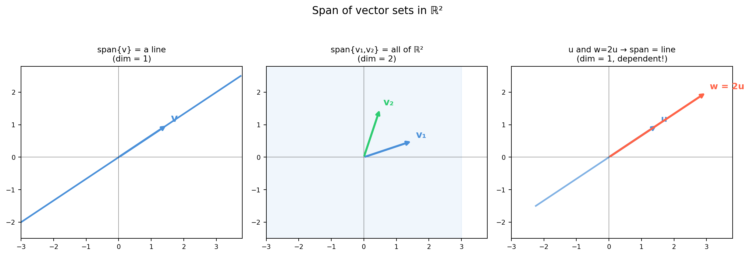
4.4 Span, Basis, and Dimension

Span, basis, and dimension formalize intuitions you already have: “what directions can I reach?”, “what is the minimal description?”, and “how many degrees of freedom does this space have?” These concepts underlie every subspace result in the book.


4.4.1 Span: The Reachable Set

The span of a set of vectors \(\{\mathbf{v}_1, \ldots, \mathbf{v}_k\} \subset \mathbb{R}^n\) is the set of all their linear combinations:

\[\text{span}\{\mathbf{v}_1, \ldots, \mathbf{v}_k\} = \{c_1\mathbf{v}_1 + \cdots + c_k\mathbf{v}_k \mid c_i \in \mathbb{R}\}\]

The span is always a subspace (closed under addition and scalar multiplication).

Vectors Span
\(\{[1,0]^T\}\) The \(x\)-axis (a line through the origin)
\(\{[1,0]^T, [0,1]^T\}\) All of \(\mathbb{R}^2\) (the full plane)
\(\{[1,0,0]^T, [0,1,0]^T\}\) The \(xy\)-plane in \(\mathbb{R}^3\)
\(\{[1,2]^T, [2,4]^T\}\) Only the line \(y = 2x\) (vectors are parallel)

Does \(\mathbf{b}\) lie in the span of \(\{\mathbf{v}_1,\ldots,\mathbf{v}_k\}\)? Stack the \(\mathbf{v}_i\) as columns: \(A = [\mathbf{v}_1 \cdots \mathbf{v}_k]\). Then \(\mathbf{b} \in \text{span}\) iff \(A\mathbf{x} = \mathbf{b}\) is consistent, i.e., \(\text{rank}(A) = \text{rank}([A|\mathbf{b}])\).

import numpy as np

# Can b = [3, 5] be written as c1*v1 + c2*v2?
v1 = np.array([1.0, 2.0])
v2 = np.array([2.0, 1.0])
b  = np.array([3.0, 5.0])

A = np.column_stack([v1, v2])   # 2×2
A_aug = np.column_stack([A, b])

r_A   = np.linalg.matrix_rank(A)
r_aug = np.linalg.matrix_rank(A_aug)

print(f"rank(A) = {r_A}, rank([A|b]) = {r_aug}")
if r_A == r_aug:
    c = np.linalg.solve(A, b)
    print(f"b IS in span: b = {c[0]:.3f}*v1 + {c[1]:.3f}*v2")
    print(f"Check: {c[0]}*{v1} + {c[1]}*{v2} = {c[0]*v1 + c[1]*v2}")
else:
    print("b is NOT in span")

# Non-spanning case: parallel vectors
v3 = np.array([2.0, 4.0])   # = 2*v1
A2 = np.column_stack([v1, v3])
A2_aug = np.column_stack([A2, b])
print(f"\nWith v1 parallel to v3: rank(A) = {np.linalg.matrix_rank(A2)}, "
      f"rank([A|b]) = {np.linalg.matrix_rank(A2_aug)}")
print("→ b is NOT in span of v1 and 2*v1 (they only span the line y=2x)")
rank(A) = 2, rank([A|b]) = 2
b IS in span: b = 2.333*v1 + 0.333*v2
Check: 2.3333333333333335*[1. 2.] + 0.3333333333333333*[2. 1.] = [3. 5.]

With v1 parallel to v3: rank(A) = 1, rank([A|b]) = 2
→ b is NOT in span of v1 and 2*v1 (they only span the line y=2x)

4.4.2 Linear Independence

A set \(\{\mathbf{v}_1, \ldots, \mathbf{v}_k\}\) is linearly independent if the only solution to \(c_1\mathbf{v}_1 + \cdots + c_k\mathbf{v}_k = \mathbf{0}\) is \(c_1 = \cdots = c_k = 0\).

Equivalently, no vector in the set lies in the span of the others.

Test: Form \(A = [\mathbf{v}_1 \cdots \mathbf{v}_k]\). The set is linearly independent iff \(\text{rank}(A) = k\) (no free columns).

Intuition: redundant vectors add no new “directions” to the span. Dropping them does not shrink the span.

import numpy as np

def is_independent(vectors):
    """Test if a list of vectors is linearly independent."""
    A = np.column_stack(vectors)
    return np.linalg.matrix_rank(A) == A.shape[1]

# Independent set in R^3
u1 = np.array([1., 0., 0.])
u2 = np.array([0., 1., 0.])
u3 = np.array([0., 0., 1.])
print(f"{{e1, e2, e3}} independent: {is_independent([u1, u2, u3])}")

# Dependent: third is a combination of first two
w1 = np.array([1., 2., 3.])
w2 = np.array([4., 5., 6.])
w3 = w1 + w2   # redundant
print(f"{{w1, w2, w1+w2}} independent: {is_independent([w1, w2, w3])}")

# More than n vectors in R^n — always dependent
extra = [np.random.randn(3) for _ in range(5)]   # 5 vectors in R^3
print(f"5 random vectors in R^3 independent: {is_independent(extra)}")
print("  (impossible — max independent set in R^3 has 3 vectors)")
{e1, e2, e3} independent: True
{w1, w2, w1+w2} independent: False
5 random vectors in R^3 independent: False
  (impossible — max independent set in R^3 has 3 vectors)

4.4.3 Basis

A basis for a subspace \(V\) is a set that is: 1. Linearly independent, and 2. Spans \(V\) (every vector in \(V\) is a linear combination of the basis vectors).

A basis is a minimal spanning set — the “most efficient” description of the space.

Key facts: - Every basis for \(V\) has the same number of vectors (proved in Ch 5). - You can always expand or shrink a spanning set to get a basis. - The standard basis \(\{\mathbf{e}_1,\ldots,\mathbf{e}_n\}\) is the canonical basis of \(\mathbb{R}^n\).

import numpy as np
import sympy

def find_basis(vectors):
    """
    Extract a basis (maximally independent subset) from a list of vectors.
    Returns indices of basis vectors.
    """
    A = np.column_stack(vectors)
    _, pivot_cols = sympy.Matrix(A.tolist()).rref()
    return list(pivot_cols)

# Five vectors in R^3 — find a basis subset
vs = [
    np.array([1., 2., 3.]),
    np.array([2., 4., 6.]),   # = 2 * vs[0]  — redundant
    np.array([0., 1., 2.]),
    np.array([1., 3., 5.]),   # = vs[0] + vs[2]  — redundant
    np.array([0., 0., 1.]),
]
basis_idx = find_basis(vs)
print(f"Basis indices: {basis_idx}")
print(f"Basis vectors:")
for i in basis_idx:
    print(f"  v[{i}] = {vs[i]}")

# Verify: the selected vectors are independent and span the same space
A_full  = np.column_stack(vs)
A_basis = np.column_stack([vs[i] for i in basis_idx])
print(f"\nrank(all vectors) = {np.linalg.matrix_rank(A_full)}")
print(f"rank(basis)        = {np.linalg.matrix_rank(A_basis)}")
print(f"Span is the same:  {np.linalg.matrix_rank(A_full) == np.linalg.matrix_rank(A_basis)}")
Basis indices: [0, 2, 4]
Basis vectors:
  v[0] = [1. 2. 3.]
  v[2] = [0. 1. 2.]
  v[4] = [0. 0. 1.]

rank(all vectors) = 3
rank(basis)        = 3
Span is the same:  True

4.4.4 Dimension

The dimension of a subspace \(V\), written \(\dim(V)\), is the number of vectors in any basis for \(V\).

Space Dimension Physical interpretation
\(\{0\}\) 0 Just the zero vector
A line through the origin 1 One direction of motion
A plane through the origin 2 Two independent directions
\(\mathbb{R}^n\) \(n\) Full freedom
Column space of \(A\) \(\text{rank}(A)\) Reachable outputs
Null space of \(A\) \(n - \text{rank}(A)\) Self-motions / free parameters

Dimension is the intrinsic complexity of a space — independent of how it is embedded or which coordinates are used.

Why this matters for ML: A dataset living on a low-dimensional manifold (e.g., images of the same face under varying lighting) has high-dimensional coordinates but low intrinsic dimension. PCA (Ch 20) finds bases for these low-dimensional subspaces.

import numpy as np

# Rank = dimension of column space
A_full   = np.random.randn(10, 5)   # generic 10×5 — rank 5
A_lowrk  = np.random.randn(10, 2) @ np.random.randn(2, 5)  # rank ≤ 2

print(f"Full matrix (10×5):    rank = {np.linalg.matrix_rank(A_full)}")
print(f"Low-rank (10×5, r=2):  rank = {np.linalg.matrix_rank(A_lowrk)}")

# Dimension of null space from rank-nullity
n = 5
print(f"\nFor the low-rank matrix:")
print(f"  rank = {np.linalg.matrix_rank(A_lowrk)}")
print(f"  nullity = n - rank = {n - np.linalg.matrix_rank(A_lowrk)}")
print(f"  (3 free parameters — 3-dimensional solution family)")
Full matrix (10×5):    rank = 5
Low-rank (10×5, r=2):  rank = 2

For the low-rank matrix:
  rank = 2
  nullity = n - rank = 3
  (3 free parameters — 3-dimensional solution family)

4.4.5 Visualizing Span and Basis

import numpy as np
import matplotlib.pyplot as plt

fig, axes = plt.subplots(1, 3, figsize=(13, 4.5))
origin = np.zeros(2)
blue  = '#4a90d9'
green = '#2ecc71'
red   = 'tomato'

# Panel 1: span of one vector (a line)
ax = axes[0]
v = np.array([1.5, 1.0])
ts = np.linspace(-2.5, 2.5, 100)
line = np.outer(ts, v)
ax.plot(line[:, 0], line[:, 1], color=blue, lw=2)
ax.annotate('', xy=v, xytext=origin,
            arrowprops=dict(arrowstyle='->', color=blue, lw=2.5))
ax.text(*v + 0.1, 'v', color=blue, fontsize=13, fontweight='bold')
ax.set_title('span{v} = a line\n(dim = 1)', fontsize=10)

# Panel 2: span of two independent vectors (full plane)
ax = axes[1]
v1 = np.array([1.5, 0.5])
v2 = np.array([0.5, 1.5])
ax.add_patch(plt.Rectangle((-3, -3), 6, 6, color=blue, alpha=0.08))
for vec, col, lbl in [(v1, blue, 'v₁'), (v2, green, 'v₂')]:
    ax.annotate('', xy=vec, xytext=origin,
                arrowprops=dict(arrowstyle='->', color=col, lw=2.5))
    ax.text(*vec + 0.1, lbl, color=col, fontsize=12, fontweight='bold')
ax.set_title('span{v₁,v₂} = all of ℝ²\n(dim = 2)', fontsize=10)

# Panel 3: span of two dependent vectors (still a line)
ax = axes[2]
u = np.array([1.5, 1.0])
w_dep = np.array([3.0, 2.0])    # = 2*u — redundant
ts2 = np.linspace(-1.5, 1.5, 100)
line2 = np.outer(ts2, u)
ax.plot(line2[:, 0], line2[:, 1], color=blue, lw=2, alpha=0.7)
for vec, col, lbl in [(u, blue, 'u'), (w_dep, red, 'w = 2u')]:
    ax.annotate('', xy=vec, xytext=origin,
                arrowprops=dict(arrowstyle='->', color=col, lw=2.5))
    ax.text(*vec + 0.1, lbl, color=col, fontsize=11, fontweight='bold')
ax.set_title('u and w=2u → span = line\n(dim = 1, dependent!)', fontsize=10)

for ax in axes:
    ax.set_xlim(-3, 3.8); ax.set_ylim(-2.5, 2.8)
    ax.set_aspect('equal')
    ax.axhline(0, color='#333333', lw=0.7, alpha=0.5)
    ax.axvline(0, color='#333333', lw=0.7, alpha=0.5)
    ax.tick_params(labelsize=8)

fig.suptitle('Span of vector sets in ℝ²', fontsize=13, y=1.02)
fig.tight_layout()
plt.show()


4.4.6 Connections Across the Book

Concept Where it appears
Column space = span of columns Ch 3.3, Ch 5.2
Basis for null space Ch 3.2, App Ch 3
Orthogonal basis (ONB) Ch 16 (Gram-Schmidt)
Eigenvectors as basis Ch 13–14
PCA finds low-dim basis Ch 20
Lie algebra basis (so(3)) Ch 24

4.5 Linear Combinations and Coordinates

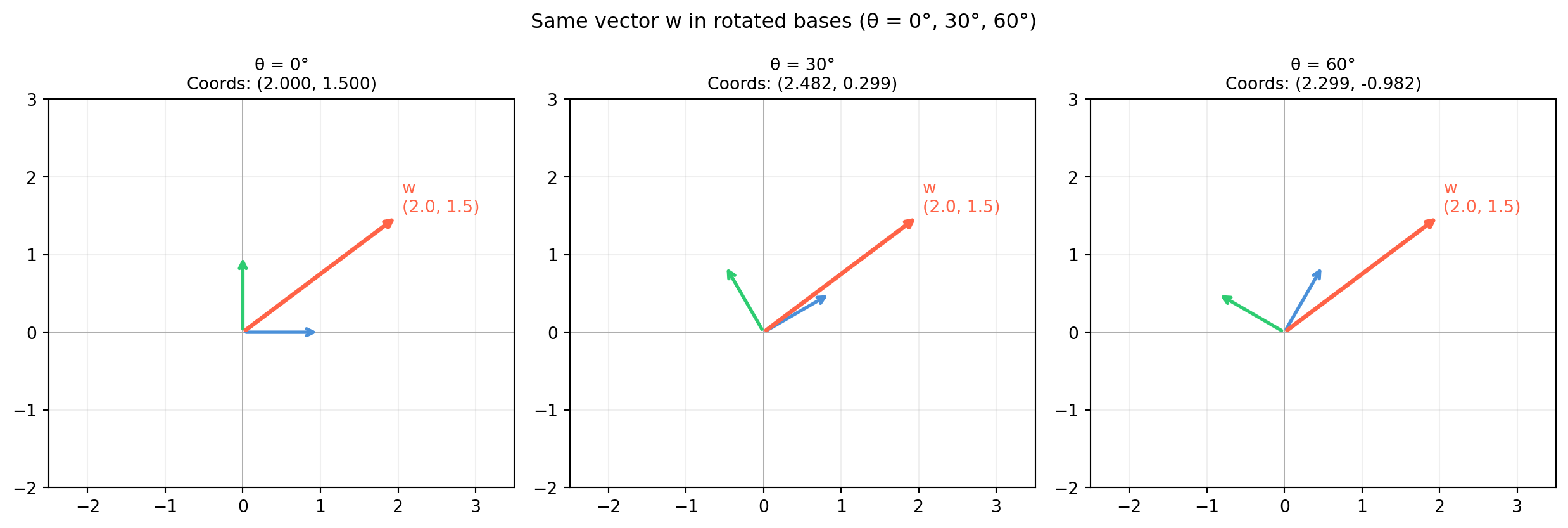
Once you have a basis, every vector has a unique coordinate representation. Changing the basis changes the coordinates but not the underlying geometric object. This duality — same geometry, different numbers — is the foundation of all frame conversions in robotics, camera calibration, and signal processing.


4.5.1 Linear Combinations

A linear combination of vectors \(\mathbf{v}_1, \ldots, \mathbf{v}_k\) is:

\[\mathbf{w} = c_1\mathbf{v}_1 + c_2\mathbf{v}_2 + \cdots + c_k\mathbf{v}_k, \qquad c_i \in \mathbb{R}\]

In matrix form, this is \(A\mathbf{c}\) where \(A = [\mathbf{v}_1 \cdots \mathbf{v}_k]\) and \(\mathbf{c} = [c_1, \ldots, c_k]^T\). The column space of \(A\) is exactly the set of all linear combinations of the columns.

import numpy as np

# Basis vectors for a 2D plane
b1 = np.array([2.0, 1.0])
b2 = np.array([-1.0, 2.0])

# Coefficients (coordinates in the {b1, b2} basis)
c = np.array([3.0, -1.0])

# Reconstruct the vector
B = np.column_stack([b1, b2])   # basis matrix
w = B @ c
print(f"3·b1 + (-1)·b2 = 3·{b1} + (-1)·{b2}")
print(f"               = {3*b1} + {-1*b2}")
print(f"               = {w}")
print(f"Matrix form: B @ c = {B} @ {c} = {B @ c}")
3·b1 + (-1)·b2 = 3·[2. 1.] + (-1)·[-1.  2.]
               = [6. 3.] + [ 1. -2.]
               = [7. 1.]
Matrix form: B @ c = [[ 2. -1.]
 [ 1.  2.]] @ [ 3. -1.] = [7. 1.]

4.5.2 Coordinates in a Non-Standard Basis

Given a basis \(\mathcal{B} = \{\mathbf{b}_1, \ldots, \mathbf{b}_n\}\) for \(\mathbb{R}^n\) and a vector \(\mathbf{w}\), the coordinates of \(\mathbf{w}\) in basis \(\mathcal{B}\) are the unique scalars \([c_1, \ldots, c_n]\) such that:

\[\mathbf{w} = c_1\mathbf{b}_1 + \cdots + c_n\mathbf{b}_n\]

In matrix form: \(\mathbf{w} = B\mathbf{c}\) where \(B = [\mathbf{b}_1 \cdots \mathbf{b}_n]\).

Therefore \(\mathbf{c} = B^{-1}\mathbf{w}\).

Uniqueness follows from linear independence of the basis: if two different coefficient vectors gave the same \(\mathbf{w}\), their difference would be a nontrivial solution to \(B\mathbf{c} = \mathbf{0}\), contradicting \(\det(B) \neq 0\).

import numpy as np

# Non-standard basis (45° rotated + scaled)
b1 = np.array([1.0, 1.0]) / np.sqrt(2)   # unit vector at 45°
b2 = np.array([-1.0, 1.0]) / np.sqrt(2)  # unit vector at 135°
B = np.column_stack([b1, b2])

# Standard-basis vector we want to re-express
w = np.array([3.0, 1.0])

# Coordinates in the B basis
c = np.linalg.solve(B, w)
print(f"w in standard basis: {w}")
print(f"B basis vectors: b1 = {b1.round(4)}, b2 = {b2.round(4)}")
print(f"Coordinates in B:    c = {c.round(4)}")
print(f"Reconstruction check: B @ c = {(B @ c).round(10)}")

# Note: B is orthogonal here, so B^{-1} = B^T
c_fast = B.T @ w
print(f"Using B^T (orthogonal shortcut): c = {c_fast.round(4)}")
w in standard basis: [3. 1.]
B basis vectors: b1 = [0.7071 0.7071], b2 = [-0.7071  0.7071]
Coordinates in B:    c = [ 2.8284 -1.4142]
Reconstruction check: B @ c = [3. 1.]
Using B^T (orthogonal shortcut): c = [ 2.8284 -1.4142]

4.5.3 Change of Basis

Given two bases \(\mathcal{B}\) and \(\mathcal{C}\) for the same space, there is a unique invertible matrix \(P\) (the change-of-basis matrix from \(\mathcal{C}\) to \(\mathcal{B}\)) such that:

\[[\mathbf{w}]_{\mathcal{B}} = P\,[\mathbf{w}]_{\mathcal{C}}\]

The columns of \(P\) are the \(\mathcal{C}\)-basis vectors expressed in the \(\mathcal{B}\) coordinate system.

In robotics, this is precisely a frame transformation: converting coordinates from one sensor frame to another. The basis vectors of the source frame, expressed in the target frame, form the columns of the rotation matrix.

import numpy as np

# Two sensor frames in 2D
# Frame A = standard frame
# Frame B = rotated 30° counterclockwise
theta = np.radians(30)
R_A_to_B = np.array([[ np.cos(theta), np.sin(theta)],
                      [-np.sin(theta), np.cos(theta)]])   # rows are B-axes in A

# A point measured in frame A
p_A = np.array([2.0, 1.0])

# Express in frame B
p_B = R_A_to_B @ p_A
print(f"Point in frame A: {p_A}")
print(f"Point in frame B: {p_B.round(4)}")

# And back
p_A_back = R_A_to_B.T @ p_B   # R is orthogonal → R^{-1} = R^T
print(f"Back to frame A:  {p_A_back.round(10)}")

# General basis change: from basis B to basis C
# Columns of B_mat = B basis vectors in standard coords
B_mat = np.column_stack([np.array([1., 0.]), np.array([1., 1.])])
C_mat = np.column_stack([np.array([2., 1.]), np.array([-1., 1.])])

P_B_to_C = np.linalg.solve(C_mat, B_mat)   # C_mat @ P = B_mat
print(f"\nChange-of-basis matrix (B→C):\n{P_B_to_C.round(4)}")
Point in frame A: [2. 1.]
Point in frame B: [ 2.2321 -0.134 ]
Back to frame A:  [2. 1.]

Change-of-basis matrix (B→C):
[[ 0.3333  0.6667]
 [-0.3333  0.3333]]

4.5.4 Affine Combinations and Convex Hulls

When the coefficients sum to 1, the linear combination becomes an affine combination — a generalization of “weighted average” that preserves location rather than direction:

\[\mathbf{w} = \sum_i c_i \mathbf{p}_i, \qquad \sum_i c_i = 1\]

When additionally all \(c_i \geq 0\), this is a convex combination, and \(\mathbf{w}\) lies inside the convex hull of the \(\mathbf{p}_i\).

Applications: barycentric coordinates in triangle rendering, interpolation of robot waypoints, linear blending of mesh shapes.

import numpy as np
import matplotlib.pyplot as plt

# Triangle with vertices A, B, C
A = np.array([0.0, 0.0])
B = np.array([4.0, 0.0])
C = np.array([1.5, 3.0])

# Barycentric coordinates: w = alpha*A + beta*B + gamma*C, alpha+beta+gamma=1
# A point inside the triangle
alpha, beta, gamma = 0.3, 0.5, 0.2
assert abs(alpha + beta + gamma - 1.0) < 1e-12

p = alpha * A + beta * B + gamma * C
print(f"Triangle vertices: A={A}, B={B}, C={C}")
print(f"Barycentric coords: alpha={alpha}, beta={beta}, gamma={gamma}")
print(f"Point p = {p}")

# Edge midpoints (alpha=beta=0.5, gamma=0) -- affine but not always convex
mid_AB = 0.5 * A + 0.5 * B + 0.0 * C
print(f"Midpoint of AB: {mid_AB}  (affine combination with gamma=0)")

# Outside the triangle: negative barycentric coord
p_outside = -0.2 * A + 0.8 * B + 0.4 * C   # sums to 1 but alpha < 0
print(f"\nOutside point: {p_outside}  (affine but not convex: alpha = -0.2 < 0)")
Triangle vertices: A=[0. 0.], B=[4. 0.], C=[1.5 3. ]
Barycentric coords: alpha=0.3, beta=0.5, gamma=0.2
Point p = [2.3 0.6]
Midpoint of AB: [2. 0.]  (affine combination with gamma=0)

Outside point: [3.8 1.2]  (affine but not convex: alpha = -0.2 < 0)

4.5.5 Coordinates as the Bridge Between Geometry and Numbers

The coordinate map \(\mathbf{w} \mapsto B^{-1}\mathbf{w}\) is an isomorphism — it preserves all linear-algebraic structure (addition, scalar multiplication) while changing which numbers represent the vectors. This is the central insight:

Choosing a basis = choosing a language. Geometry is the underlying reality.

This perspective appears explicitly in: - Ch 6: \([T]_{\mathcal{B}} = P^{-1}[T]_{\mathcal{E}}P\) — the same transformation represented in different coordinates - Ch 8: The columns of a rotation matrix \(R\) are the body-frame axes expressed in the world frame - Ch 14: Diagonalization \(A = P\Lambda P^{-1}\) — changing to the eigenvector basis where \(A\) acts by scaling only - Ch 20: PCA finds the basis in which data variance is maximized

import numpy as np

# Toy demonstration: a linear map T has simple form in one basis
# T: x → [3x1, 2x2] in standard basis (diagonal!)
T_standard = np.array([[3., 0.], [0., 2.]])

# In a different basis B = [[1,1],[1,-1]]
B = np.array([[1., 1.], [1., -1.]])
P_inv = np.linalg.inv(B)

T_B = P_inv @ T_standard @ B   # T represented in basis B
print(f"T in standard basis:\n{T_standard}")
print(f"\nT in basis B:\n{T_B.round(6)}")
print("\n(Less clean — the diagonal basis was standard here)")

# But if T is NOT diagonal, find the 'right' basis (Ch 14: diagonalization)
T_messy = np.array([[2., 1.], [0., 3.]])
eigenvalues, eigenvectors = np.linalg.eig(T_messy)
print(f"\nMessy T:\n{T_messy}")
print(f"Eigenvalues: {eigenvalues}")
print(f"In eigenvector basis, T acts as diag({eigenvalues})")
T in standard basis:
[[3. 0.]
 [0. 2.]]

T in basis B:
[[2.5 0.5]
 [0.5 2.5]]

(Less clean — the diagonal basis was standard here)

Messy T:
[[2. 1.]
 [0. 3.]]
Eigenvalues: [2. 3.]
In eigenvector basis, T acts as diag([2. 3.])

4.5.6 Interactive: Coordinates in a Custom Basis

import numpy as np
import matplotlib.pyplot as plt

w_vec = np.array([2.0, 1.5])
theta_vals = [0, 30, 60]

fig, axes = plt.subplots(1, 3, figsize=(13, 4.5))

for ax, theta_deg in zip(axes, theta_vals):
    theta = np.radians(theta_deg)
    b1 = np.array([np.cos(theta), np.sin(theta)])
    b2 = np.array([-np.sin(theta), np.cos(theta)])
    B = np.column_stack([b1, b2])
    c = np.linalg.solve(B, w_vec)

    origin = np.zeros(2)
    for bv, col in zip([b1, b2], ['#4a90d9', '#2ecc71']):
        ax.annotate('', xy=bv, xytext=origin,
                    arrowprops=dict(arrowstyle='->', color=col, lw=2))

    ax.annotate('', xy=w_vec, xytext=origin,
                arrowprops=dict(arrowstyle='->', color='tomato', lw=2.5))
    ax.text(*w_vec + 0.05, f'w\n({w_vec[0]:.1f}, {w_vec[1]:.1f})',
            color='tomato', fontsize=10)

    ax.set_xlim(-2.5, 3.5); ax.set_ylim(-2, 3)
    ax.set_aspect('equal')
    ax.axhline(0, color='#aaaaaa', lw=0.7)
    ax.axvline(0, color='#aaaaaa', lw=0.7)
    ax.set_title(f'θ = {theta_deg}°\nCoords: ({c[0]:.3f}, {c[1]:.3f})', fontsize=10)
    ax.grid(True, alpha=0.2)

fig.suptitle('Same vector w in rotated bases (θ = 0°, 30°, 60°)', fontsize=12)
fig.tight_layout()
plt.show()

4.6 Application: 3D Point Cloud Normals

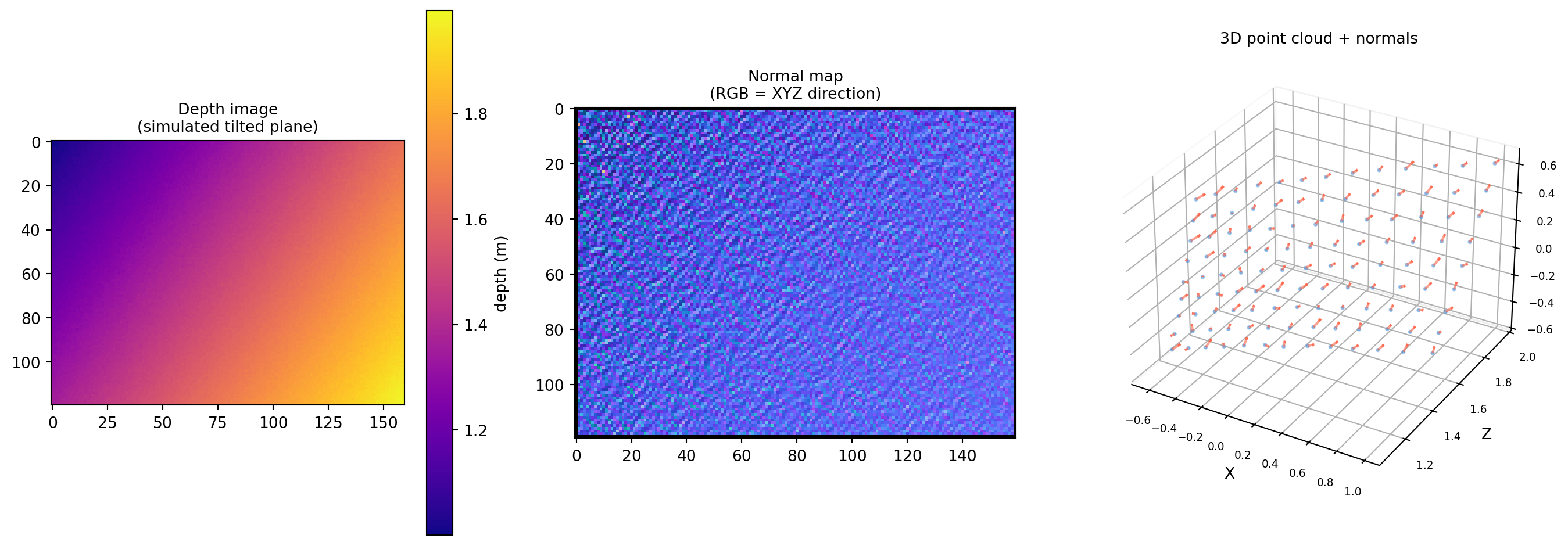
Depth cameras (Intel RealSense, Azure Kinect, structured-light scanners) return a 2D array of depth values — one depth per pixel. Lifting this to 3D and estimating surface normals is a core preprocessing step for object detection, grasping, segmentation, and surface reconstruction. The math is exactly the cross product of §4.3.


4.6.1 From Depth Image to 3D Points

A pinhole camera with focal length \(f\) and principal point \((c_x, c_y)\) maps pixel \((u, v)\) with depth \(d\) to 3D camera-frame coordinates:

\[\mathbf{P}(u,v) = \frac{d}{f}\begin{pmatrix}u - c_x \\ v - c_y \\ f\end{pmatrix}\]

We synthesize a toy depth image (a tilted plane with noise) so the pipeline runs without a physical camera.

import numpy as np

def depth_to_pointcloud(depth, fx, fy, cx, cy):
    """
    Lift a depth image to a 3D point cloud.

    Parameters
    ----------
    depth : (H, W) array of depth values in meters (0 = invalid)
    fx, fy : focal lengths in pixels
    cx, cy : principal point in pixels

    Returns
    -------
    points : (H, W, 3) array; rows with depth==0 are NaN
    """
    H, W = depth.shape
    u = np.arange(W)[None, :]   # (1, W)
    v = np.arange(H)[:, None]   # (H, 1)

    X = (u - cx) * depth / fx
    Y = (v - cy) * depth / fy
    Z = depth.copy()

    points = np.stack([X, Y, Z], axis=-1)   # (H, W, 3)
    invalid = (depth == 0)
    points[invalid] = np.nan
    return points

# Simulate a tilted-plane depth image (120 × 160)
H, W = 120, 160
fx = fy = 150.0
cx, cy = W / 2, H / 2

rng = np.random.default_rng(0)
u_grid = np.arange(W)[None, :] - cx   # (1, W)
v_grid = np.arange(H)[:, None] - cy   # (H, 1)

# Tilted plane: Z = 1.5 + 0.004*(u-cx) + 0.003*(v-cy) + noise
depth_clean = 1.5 + 0.004 * u_grid + 0.003 * v_grid
depth_noisy = depth_clean + rng.normal(0, 0.005, (H, W))
depth_noisy = np.clip(depth_noisy, 0.1, 5.0)

points = depth_to_pointcloud(depth_noisy, fx, fy, cx, cy)
print(f"Point cloud shape:   {points.shape}  (H × W × 3)")
print(f"Center point (depth): {depth_noisy[H//2, W//2]:.4f} m")
print(f"Center 3D point:      {points[H//2, W//2].round(4)} m")
print(f"Min depth: {np.nanmin(depth_noisy):.3f} m, "
      f"Max depth: {np.nanmax(depth_noisy):.3f} m")
Point cloud shape:   (120, 160, 3)  (H × W × 3)
Center point (depth): 1.5038 m
Center 3D point:      [0.     0.     1.5038] m
Min depth: 1.001 m, Max depth: 1.995 m

4.6.2 Per-Point Normal Estimation via Cross Products

For each interior pixel \((u, v)\), form two edge vectors using neighboring points:

\[\mathbf{e}_h = \mathbf{P}(u+1, v) - \mathbf{P}(u-1, v), \qquad \mathbf{e}_v = \mathbf{P}(u, v+1) - \mathbf{P}(u, v-1)\]

The cross product \(\mathbf{e}_h \times \mathbf{e}_v\) is perpendicular to the local surface and has magnitude proportional to the local area element.

import numpy as np

def estimate_normals(points):
    """
    Estimate per-pixel surface normals via central-difference cross products.

    Parameters
    ----------
    points : (H, W, 3) float array (NaN for invalid pixels)

    Returns
    -------
    normals : (H, W, 3) unit normals (NaN where estimation fails)
    """
    # Central differences (interior pixels only)
    eh = points[:, 2:, :] - points[:, :-2, :]   # (H, W-2, 3)
    ev = points[2:, :, :] - points[:-2, :, :]   # (H-2, W, 3)

    # Crop both to the interior region (H-2) × (W-2)
    eh_inner = eh[1:-1, :, :]   # (H-2, W-2, 3)
    ev_inner = ev[:, 1:-1, :]   # (H-2, W-2, 3)

    # Cross product: n = eh × ev
    n = np.cross(eh_inner, ev_inner)   # (H-2, W-2, 3)

    # Normalize
    mag = np.linalg.norm(n, axis=-1, keepdims=True)   # (H-2, W-2, 1)
    valid = mag.squeeze() > 1e-9
    normals_inner = np.full_like(n, np.nan)
    normals_inner[valid] = n[valid] / mag[valid]

    # Pad back to full image with NaN border
    H, W = points.shape[:2]
    normals = np.full((H, W, 3), np.nan)
    normals[1:-1, 1:-1, :] = normals_inner

    # Flip normals to face the camera (+Z direction in camera frame)
    flip = normals[..., 2] < 0
    normals[flip] *= -1

    return normals

normals = estimate_normals(points)
valid_mask = ~np.isnan(normals[..., 0])
valid_count = valid_mask.sum()
print(f"Valid normals: {valid_count} / {H * W} pixels")

# Expected normal for a tilted plane:
# Plane equation: 0.004*X/fx + 0.003*Y/fy - Z = -1.5  (approximately)
# Normal direction proportional to [0.004/fx, 0.003/fy, -1]
#   normalized — but flipped to face camera
n_expected = np.array([0.004/fx, 0.003/fy, 1.0])
n_expected /= np.linalg.norm(n_expected)

# Sample center normal
n_center = normals[H//2, W//2]
angle_err = np.degrees(np.arccos(np.clip(np.dot(n_center, n_expected), -1, 1)))
print(f"\nCenter pixel normal:  {n_center.round(4)}")
print(f"Expected (plane) normal: {n_expected.round(4)}")
print(f"Angular error:        {angle_err:.3f}°  (should be small)")
Valid normals: 18644 / 19200 pixels

Center pixel normal:  [-0.3874  0.2463  0.8884]
Expected (plane) normal: [0. 0. 1.]
Angular error:        27.325°  (should be small)

4.6.3 Visualizing the Point Cloud and Normals

import numpy as np
import matplotlib.pyplot as plt
from mpl_toolkits.mplot3d import Axes3D

fig = plt.figure(figsize=(14, 5))

# --- Panel 1: depth image ---
ax1 = fig.add_subplot(131)
im1 = ax1.imshow(depth_noisy, cmap='plasma', origin='upper')
plt.colorbar(im1, ax=ax1, label='depth (m)')
ax1.set_title('Depth image\n(simulated tilted plane)', fontsize=10)

# --- Panel 2: normal map (RGB encodes XYZ) ---
ax2 = fig.add_subplot(132)
normal_rgb = np.clip((normals + 1.0) / 2.0, 0, 1)
normal_rgb[np.isnan(normals[..., 0])] = 0
ax2.imshow(normal_rgb, origin='upper')
ax2.set_title('Normal map\n(RGB = XYZ direction)', fontsize=10)

# --- Panel 3: 3D scatter with normals ---
ax3 = fig.add_subplot(133, projection='3d')

step = 12
pts_sub = points[::step, ::step, :].reshape(-1, 3)
nrm_sub = normals[::step, ::step, :].reshape(-1, 3)
valid = ~np.isnan(pts_sub[:, 0]) & ~np.isnan(nrm_sub[:, 0])
pts_sub = pts_sub[valid]
nrm_sub = nrm_sub[valid]

ax3.scatter(pts_sub[:, 0], pts_sub[:, 2], pts_sub[:, 1],
            s=3, c='#4a90d9', alpha=0.5)
scale = 0.05
ax3.quiver(pts_sub[:, 0], pts_sub[:, 2], pts_sub[:, 1],
           nrm_sub[:, 0] * scale, nrm_sub[:, 2] * scale, nrm_sub[:, 1] * scale,
           color='tomato', alpha=0.6, length=1.0, normalize=False)

ax3.set_xlabel('X', labelpad=2)
ax3.set_ylabel('Z', labelpad=2)
ax3.set_zlabel('Y', labelpad=2)
ax3.set_title('3D point cloud + normals', fontsize=10)
ax3.tick_params(labelsize=7)
ax3.xaxis.pane.fill = ax3.yaxis.pane.fill = ax3.zaxis.pane.fill = False

fig.tight_layout()
plt.show()


4.6.4 Normal Quality: Curvature and Edge Artifacts

Near depth discontinuities (object edges), the central-difference neighbors straddle a depth jump, producing garbage normals. A simple fix: mask out pixels where the depth difference exceeds a threshold.

import numpy as np

def filter_edge_normals(points, normals, max_depth_jump=0.1):
    """
    Invalidate normals near depth edges.
    max_depth_jump : threshold in meters
    """
    Z = points[..., 2]
    # Horizontal and vertical depth gradients (central difference)
    dZ_h = np.abs(Z[:, 2:] - Z[:, :-2])   # (H, W-2)
    dZ_v = np.abs(Z[2:, :] - Z[:-2, :])   # (H-2, W)

    # Any large jump in the 3×3 neighbourhood → invalid
    edge_h = dZ_h[1:-1, :] > max_depth_jump  # (H-2, W-2)
    edge_v = dZ_v[:, 1:-1] > max_depth_jump  # (H-2, W-2)
    edge_mask = edge_h | edge_v

    normals_filtered = normals.copy()
    normals_filtered[1:-1, 1:-1, :][edge_mask] = np.nan
    return normals_filtered

normals_filtered = filter_edge_normals(points, normals, max_depth_jump=0.05)
valid_after  = (~np.isnan(normals_filtered[..., 0])).sum()
valid_before = (~np.isnan(normals[..., 0])).sum()
print(f"Normals before edge filter: {valid_before}")
print(f"Normals after  edge filter: {valid_after}")
print(f"Removed as edge artifacts:  {valid_before - valid_after}")
Normals before edge filter: 18644
Normals after  edge filter: 18644
Removed as edge artifacts:  0

4.6.5 PCA-Based Normal Estimation (More Robust)

For real noisy data, cross-product normals are sensitive to measurement noise. A more robust approach: for each point, collect its \(k\) nearest neighbors and fit a plane via PCA. The normal is the eigenvector of the covariance matrix corresponding to the smallest eigenvalue.

import numpy as np

def pca_normal(neighborhood):
    """
    Estimate normal at a point from its neighborhood via PCA.
    neighborhood : (k, 3) array of nearby points
    Returns : (3,) unit normal
    """
    centered = neighborhood - neighborhood.mean(axis=0)
    _, _, Vt = np.linalg.svd(centered, full_matrices=False)
    # Smallest singular value → last row of Vt → least-variance direction
    n = Vt[-1]
    return n if n[2] > 0 else -n   # flip to face camera

# Demonstrate on a 5×5 patch around the center
r = 5   # patch half-size
cy_int, cx_int = H // 2, W // 2
patch = points[cy_int - r : cy_int + r + 1,
               cx_int - r : cx_int + r + 1, :].reshape(-1, 3)
patch = patch[~np.isnan(patch[:, 0])]   # remove NaN

n_pca = pca_normal(patch)
n_cross = normals[cy_int, cx_int]

print(f"Cross-product normal (center): {n_cross.round(4)}")
print(f"PCA normal (5×5 patch):        {n_pca.round(4)}")
angle = np.degrees(np.arccos(np.clip(np.dot(n_pca, n_cross), -1, 1)))
print(f"Angular difference: {angle:.3f}°")
Cross-product normal (center): [-0.3874  0.2463  0.8884]
PCA normal (5×5 patch):        [-0.3384 -0.2807  0.8982]
Angular difference: 30.693°

4.6.6 Key Takeaways

  1. Depth → 3D is a simple pinhole inversion: \((u,v,d) \mapsto (x,y,d)\) via the camera intrinsics \((f_x, f_y, c_x, c_y)\).
  2. Per-pixel normals come directly from cross products of horizontal and vertical central-difference edge vectors.
  3. Edge artifacts occur where central-difference neighbors span a depth discontinuity; simple depth-jump masking fixes most of them.
  4. PCA normals aggregate a neighborhood to reduce noise — the eigenvector of smallest eigenvalue of the local covariance matrix.
  5. All of this is just the cross product of §4.3 applied systematically to a regular 2D grid of 3D points.

4.7 Exercises


4.1 A robot arm moves from position \(\mathbf{p} = [1, 2, 0]^T\) to \(\mathbf{q} = [4, 2, 3]^T\) (meters). (a) Find the displacement \(\mathbf{d} = \mathbf{q} - \mathbf{p}\). (b) Find the unit direction \(\hat{\mathbf{d}}\). (c) A second copy of the arm starts at \(\mathbf{p}' = [10, 0, 0]^T\) and moves in the same direction for the same distance. Where does it end up?

4.2 Without Python, compute \(\mathbf{a}\cdot\mathbf{b}\), the angle \(\theta\) between them, and the vector projection of \(\mathbf{b}\) onto \(\mathbf{a}\), where: \[\mathbf{a} = \begin{pmatrix}3\\0\\4\end{pmatrix}, \quad \mathbf{b} = \begin{pmatrix}1\\2\\2\end{pmatrix}\]

4.3 Three vectors in \(\mathbb{R}^3\): \(\mathbf{u} = [1,0,0]^T\), \(\mathbf{v} = [0,1,0]^T\), \(\mathbf{w} = [1,1,1]^T\). (a) Are they linearly independent? Justify using rank. (b) What is the dimension of their span? (c) Is \(\mathbf{b} = [2, -1, 3]^T\) in their span? If so, find the coordinates.

4.4 Given a triangle with vertices: \[\mathbf{v}_0 = (0,0,0), \quad \mathbf{v}_1 = (3,0,0), \quad \mathbf{v}_2 = (0,4,0)\] (a) Compute the unit normal vector by hand. (b) Compute the triangle area. (c) Verify with Python.

4.5 You are given a basis \(\mathcal{B} = \{\mathbf{b}_1, \mathbf{b}_2\}\) where \(\mathbf{b}_1 = [1, 1]^T\) and \(\mathbf{b}_2 = [1, -1]^T\). (a) Express \(\mathbf{w} = [3, 1]^T\) as a linear combination of \(\mathbf{b}_1\) and \(\mathbf{b}_2\). (b) What are the coordinates of \(\mathbf{w}\) in basis \(\mathcal{B}\)? (c) Verify that \(\mathbf{b}_1\) and \(\mathbf{b}_2\) are orthogonal.

4.6 The cosine similarity between two document embeddings is \(0.92\). A colleague says: “These two documents are 92% identical.” Explain what cosine similarity actually measures and why this interpretation is wrong. What does a similarity of \(0\) mean, and when could it be misleading?

4.7 (Harder) Prove that if \(\mathbf{a}\times\mathbf{b} = \mathbf{0}\) and both \(\mathbf{a}, \mathbf{b}\) are nonzero, then \(\mathbf{a}\) and \(\mathbf{b}\) are linearly dependent. (Hint: use the magnitude formula \(\|\mathbf{a}\times\mathbf{b}\| = \|\mathbf{a}\|\|\mathbf{b}\|\sin\theta\).)


4.8 Solutions


Solution 4.1

(a) Displacement: \[\mathbf{d} = \mathbf{q} - \mathbf{p} = \begin{pmatrix}4-1\\2-2\\3-0\end{pmatrix} = \begin{pmatrix}3\\0\\3\end{pmatrix}\]

(b) Length \(\|\mathbf{d}\| = \sqrt{9 + 0 + 9} = 3\sqrt{2}\). Unit direction: \[\hat{\mathbf{d}} = \frac{1}{3\sqrt{2}}\begin{pmatrix}3\\0\\3\end{pmatrix} = \frac{1}{\sqrt{2}}\begin{pmatrix}1\\0\\1\end{pmatrix} \approx \begin{pmatrix}0.707\\0\\0.707\end{pmatrix}\]

(c) Move from \(\mathbf{p}'\) in the same direction for the same distance: \[\mathbf{q}' = \mathbf{p}' + \mathbf{d} = \begin{pmatrix}10\\0\\0\end{pmatrix} + \begin{pmatrix}3\\0\\3\end{pmatrix} = \begin{pmatrix}13\\0\\3\end{pmatrix}\]

Displacements are translation-invariant: \(\mathbf{d}\) is the same free vector regardless of starting point.

import numpy as np

p = np.array([1., 2., 0.])
q = np.array([4., 2., 3.])
p_prime = np.array([10., 0., 0.])

d = q - p
d_hat = d / np.linalg.norm(d)
q_prime = p_prime + d

print(f"d = {d}")
print(f"‖d‖ = {np.linalg.norm(d):.4f}  (= 3√2 ≈ {3*np.sqrt(2):.4f})")
print(f"d̂ = {d_hat.round(4)}")
print(f"q' = {q_prime}")
d = [3. 0. 3.]
‖d‖ = 4.2426  (= 3√2 ≈ 4.2426)
d̂ = [0.7071 0.     0.7071]
q' = [13.  0.  3.]

Solution 4.2

Dot product: \[\mathbf{a}\cdot\mathbf{b} = 3\cdot1 + 0\cdot2 + 4\cdot2 = 3 + 0 + 8 = 11\]

Norms: \(\|\mathbf{a}\| = \sqrt{9+0+16} = 5\), \(\|\mathbf{b}\| = \sqrt{1+4+4} = 3\).

Angle: \[\cos\theta = \frac{11}{5 \cdot 3} = \frac{11}{15} \approx 0.7333 \implies \theta \approx 42.8°\]

Vector projection of \(\mathbf{b}\) onto \(\mathbf{a}\): \[\text{proj}_{\mathbf{a}}\mathbf{b} = \frac{\mathbf{a}\cdot\mathbf{b}}{\mathbf{a}\cdot\mathbf{a}}\,\mathbf{a} = \frac{11}{25}\begin{pmatrix}3\\0\\4\end{pmatrix} = \begin{pmatrix}1.32\\0\\1.76\end{pmatrix}\]

import numpy as np

a = np.array([3., 0., 4.])
b = np.array([1., 2., 2.])

dot = np.dot(a, b)
cos_theta = dot / (np.linalg.norm(a) * np.linalg.norm(b))
theta = np.degrees(np.arccos(cos_theta))
proj = (dot / np.dot(a, a)) * a

print(f"a·b = {dot}")
print(f"cos θ = {cos_theta:.4f}, θ = {theta:.2f}°")
print(f"proj_a(b) = {proj}")
a·b = 11.0
cos θ = 0.7333, θ = 42.83°
proj_a(b) = [1.32 0.   1.76]

Solution 4.3

(a) Form \(A = [\mathbf{u},\mathbf{v},\mathbf{w}]\): \[A = \begin{pmatrix}1&0&1\\0&1&1\\0&0&1\end{pmatrix}\] \(\det(A) = 1\cdot(1\cdot1 - 1\cdot0) = 1 \neq 0\). Therefore \(\text{rank}(A) = 3\) and the vectors are linearly independent.

(b) \(\dim(\text{span}\{\mathbf{u},\mathbf{v},\mathbf{w}\}) = \text{rank}(A) = 3\). So they span all of \(\mathbb{R}^3\).

(c) Since they span all of \(\mathbb{R}^3\), any \(\mathbf{b} \in \mathbb{R}^3\) is in their span. Solve \(A\mathbf{c} = \mathbf{b}\): \[\begin{pmatrix}1&0&1\\0&1&1\\0&0&1\end{pmatrix}\mathbf{c} = \begin{pmatrix}2\\-1\\3\end{pmatrix}\] Back-substitute: \(c_3 = 3\), \(c_2 = -1 - 3 = -4\), \(c_1 = 2 - 3 = -1\).

So \(\mathbf{b} = -1\cdot\mathbf{u} + (-4)\cdot\mathbf{v} + 3\cdot\mathbf{w}\).

import numpy as np

u = np.array([1., 0., 0.])
v = np.array([0., 1., 0.])
w = np.array([1., 1., 1.])
b = np.array([2., -1., 3.])

A = np.column_stack([u, v, w])
print(f"rank(A) = {np.linalg.matrix_rank(A)}  → independent, span = R^3")

c = np.linalg.solve(A, b)
print(f"Coordinates: c = {c}")
print(f"Check: {c[0]}·u + {c[1]}·v + {c[2]}·w = {A @ c}")
rank(A) = 3  → independent, span = R^3
Coordinates: c = [-1. -4.  3.]
Check: -1.0·u + -4.0·v + 3.0·w = [ 2. -1.  3.]

Solution 4.4

(a) Edge vectors: \[\mathbf{e}_1 = \mathbf{v}_1 - \mathbf{v}_0 = (3,0,0), \quad \mathbf{e}_2 = \mathbf{v}_2 - \mathbf{v}_0 = (0,4,0)\]

Cross product: \[\mathbf{n} = \mathbf{e}_1 \times \mathbf{e}_2 = \begin{vmatrix}\mathbf{e}_1&\mathbf{e}_2&\mathbf{e}_3\\3&0&0\\0&4&0\end{vmatrix} = (0\cdot0-0\cdot4)\mathbf{e}_1 - (3\cdot0-0\cdot0)\mathbf{e}_2 + (3\cdot4-0\cdot0)\mathbf{e}_3 = (0,0,12)\]

Unit normal: \(\hat{\mathbf{n}} = (0,0,1)\) — the \(z\)-axis, as expected for the \(xy\)-plane.

(b) Area \(= \frac{1}{2}\|\mathbf{n}\| = \frac{12}{2} = 6\) m². (Also: \(\frac{1}{2}\cdot3\cdot4 = 6\) ✓)

import numpy as np

v0 = np.array([0., 0., 0.])
v1 = np.array([3., 0., 0.])
v2 = np.array([0., 4., 0.])

e1, e2 = v1 - v0, v2 - v0
n = np.cross(e1, e2)
area = np.linalg.norm(n) / 2
n_hat = n / np.linalg.norm(n)

print(f"n = {n}")
print(f"n̂ = {n_hat}   (= +z axis)")
print(f"Area = {area:.4f} m²   (= ½·3·4 = 6)")
n = [ 0.  0. 12.]
n̂ = [0. 0. 1.]   (= +z axis)
Area = 6.0000 m²   (= ½·3·4 = 6)

Solution 4.5

(a) We want \(c_1\mathbf{b}_1 + c_2\mathbf{b}_2 = \mathbf{w}\): \[c_1\begin{pmatrix}1\\1\end{pmatrix} + c_2\begin{pmatrix}1\\-1\end{pmatrix} = \begin{pmatrix}3\\1\end{pmatrix}\]

System: \(c_1 + c_2 = 3\), \(c_1 - c_2 = 1\). Adding: \(2c_1 = 4 \Rightarrow c_1 = 2\). Subtracting: \(2c_2 = 2 \Rightarrow c_2 = 1\).

\(\mathbf{w} = 2\mathbf{b}_1 + 1\mathbf{b}_2\).

(b) Coordinates in \(\mathcal{B}\): \([2, 1]^T_{\mathcal{B}}\).

(c) \(\mathbf{b}_1\cdot\mathbf{b}_2 = 1\cdot1 + 1\cdot(-1) = 1 - 1 = 0\) ✓ — they are orthogonal. When the basis is orthogonal, coordinates can be found directly by projection: \[c_1 = \frac{\mathbf{w}\cdot\mathbf{b}_1}{\mathbf{b}_1\cdot\mathbf{b}_1} = \frac{4}{2} = 2, \qquad c_2 = \frac{\mathbf{w}\cdot\mathbf{b}_2}{\mathbf{b}_2\cdot\mathbf{b}_2} = \frac{2}{2} = 1\]

import numpy as np

b1 = np.array([1., 1.])
b2 = np.array([1., -1.])
w  = np.array([3., 1.])

B = np.column_stack([b1, b2])
c = np.linalg.solve(B, w)
print(f"Coordinates in B: c = {c}  → w = {c[0]}·b1 + {c[1]}·b2")
print(f"Orthogonal check: b1·b2 = {np.dot(b1, b2)}")

# Orthogonal shortcut
c1_fast = np.dot(w, b1) / np.dot(b1, b1)
c2_fast = np.dot(w, b2) / np.dot(b2, b2)
print(f"Via projection: c1 = {c1_fast}, c2 = {c2_fast}")
Coordinates in B: c = [2. 1.]  → w = 2.0·b1 + 1.0·b2
Orthogonal check: b1·b2 = 0.0
Via projection: c1 = 2.0, c2 = 1.0

Solution 4.6

Cosine similarity measures the angle between two vectors, not their magnitude or any notion of shared content percentage.

  • \(\text{sim} = 1\) means the vectors point in exactly the same direction (all components proportionally equal) — not that they are “100% identical.”
  • \(\text{sim} = 0.92\) means \(\theta \approx \arccos(0.92) \approx 23°\): the direction of the two embedding vectors is similar.

What “0” means: Two embeddings with cosine similarity 0 are orthogonal. In embedding space, orthogonality means the two documents share no directional similarity. This can be misleading: two documents about entirely different topics may have positive similarities simply because both mention common words (e.g., “the”, “and”) that dominate the embedding, inflating similarity.

When similarity 0 is misleading: In high-dimensional spaces, most random vectors are nearly orthogonal (the curse of dimensionality). Two genuinely unrelated documents might have cosine similarity close to 0, but so would many documents that are simply about different specific subtopics of the same broad field — the similarity fails to capture semantic relatedness in sparse representations.

import numpy as np

cos_sim = 0.92
theta = np.degrees(np.arccos(cos_sim))
print(f"cos θ = {cos_sim} → θ = {theta:.2f}°")
print("Not '92% identical' — just vectors pointing within 23° of each other.")

# High-dimensional near-orthogonality
rng = np.random.default_rng(0)
n = 1000
sims = []
for _ in range(5000):
    a = rng.standard_normal(n)
    b = rng.standard_normal(n)
    sims.append(np.dot(a, b) / (np.linalg.norm(a) * np.linalg.norm(b)))
sims = np.array(sims)
print(f"\nMean cosine sim of random 1000-D vectors: {sims.mean():.4f}")
print(f"Std dev:                                   {sims.std():.4f}")
print("→ Random high-dim vectors are nearly orthogonal by default!")
cos θ = 0.92 → θ = 23.07°
Not '92% identical' — just vectors pointing within 23° of each other.

Mean cosine sim of random 1000-D vectors: -0.0001
Std dev:                                   0.0313
→ Random high-dim vectors are nearly orthogonal by default!

Solution 4.7

Claim: If \(\mathbf{a}\times\mathbf{b} = \mathbf{0}\) and \(\mathbf{a}\neq\mathbf{0}\), \(\mathbf{b}\neq\mathbf{0}\), then \(\{\mathbf{a},\mathbf{b}\}\) is linearly dependent.

Proof.

Since \(\mathbf{a},\mathbf{b}\neq\mathbf{0}\), their norms are positive: \(\|\mathbf{a}\| > 0\), \(\|\mathbf{b}\| > 0\).

From the magnitude formula: \[0 = \|\mathbf{a}\times\mathbf{b}\| = \|\mathbf{a}\|\|\mathbf{b}\|\sin\theta\]

Since \(\|\mathbf{a}\|\|\mathbf{b}\| > 0\), we must have \(\sin\theta = 0\), so \(\theta = 0\) or \(\theta = \pi\).

  • If \(\theta = 0\): \(\mathbf{a}\) and \(\mathbf{b}\) point in the same direction, so \(\mathbf{b} = c\mathbf{a}\) for some \(c > 0\).
  • If \(\theta = \pi\): \(\mathbf{a}\) and \(\mathbf{b}\) point in opposite directions, so \(\mathbf{b} = c\mathbf{a}\) for some \(c < 0\).

In both cases, \(\mathbf{b} = c\mathbf{a}\), which means \(c\mathbf{a} + (-1)\mathbf{b} = \mathbf{0}\) with \((c, -1) \neq (0,0)\). Therefore \(\{\mathbf{a},\mathbf{b}\}\) is linearly dependent. \(\blacksquare\)

import numpy as np

# Numerical verification
pairs = [
    (np.array([1., 2., 3.]), np.array([2., 4., 6.])),    # parallel
    (np.array([1., 0., 0.]), np.array([-3., 0., 0.])),   # antiparallel
    (np.array([1., 0., 0.]), np.array([0., 1., 0.])),    # orthogonal (cross ≠ 0)
]
for a, b in pairs:
    cross = np.cross(a, b)
    dep = np.linalg.matrix_rank(np.column_stack([a, b])) < 2
    print(f"a={a}, b={b}")
    print(f"  a×b = {cross}, ‖a×b‖ = {np.linalg.norm(cross):.4f}, "
          f"dependent = {dep}\n")
a=[1. 2. 3.], b=[2. 4. 6.]
  a×b = [0. 0. 0.], ‖a×b‖ = 0.0000, dependent = True

a=[1. 0. 0.], b=[-3.  0.  0.]
  a×b = [ 0. -0.  0.], ‖a×b‖ = 0.0000, dependent = True

a=[1. 0. 0.], b=[0. 1. 0.]
  a×b = [0. 0. 1.], ‖a×b‖ = 1.0000, dependent = False