21  Matrix Calculus

21.1 Layout Conventions

Every chapter in this book has used derivatives of matrix expressions without stopping to formalize the rules. In Ch 17 we minimized \(\|A\mathbf{x}-\mathbf{b}\|^2\) by setting its gradient to zero and obtained the normal equations \(A^TA\mathbf{x}=A^T\mathbf{b}\). In Ch 20 we set \(\partial\mathcal{L}/\partial\mathbf{u}=\mathbf{0}\) for the PCA Lagrangian and recovered \(\Sigma\mathbf{u}=\lambda\mathbf{u}\). Both steps relied on a quiet choice: the derivative of a scalar with respect to a vector is itself a column vector. That choice is one of two competing layout conventions in the literature, and mixing them silently is the source of a large fraction of backpropagation bugs.

This section makes the choice explicit and gives you the tools to translate between conventions whenever you encounter the other one.

---

21.1.1 The Two Conventions

Let \(f:\mathbb{R}^n\to\mathbb{R}\) be a differentiable scalar function and \(\mathbf{x}\in\mathbb{R}^n\).

Denominator layout (also called gradient layout or Hessian layout):

\[\frac{\partial f}{\partial \mathbf{x}} \;\stackrel{\text{def}}{=}\; \begin{pmatrix}\partial f/\partial x_1\\\vdots\\\partial f/\partial x_n\end{pmatrix} \in\mathbb{R}^{n\times 1}.\]

The result has the same shape as the denominator \(\mathbf{x}\).

Numerator layout (also called Jacobian layout):

\[\frac{\partial f}{\partial \mathbf{x}} \;\stackrel{\text{def}}{=}\; \begin{pmatrix}\partial f/\partial x_1&\cdots&\partial f/\partial x_n\end{pmatrix} \in\mathbb{R}^{1\times n}.\]

The result has the same shape as the numerator \(f\) (a \(1\times 1\) scalar treated as having one row, so the derivative gains one column per denominator element).

Convention used throughout this book: We use denominator layout for scalar-by-vector derivatives. \(\dfrac{\partial f}{\partial \mathbf{x}}\) is always a column vector, the same shape as \(\mathbf{x}\). This matches NumPy’s default array orientation, keeps gradients the same shape as parameters, and is consistent with every derivation in Ch 17 and Ch 20.

---

21.1.2 Extension to Vector Functions

Let \(\mathbf{f}:\mathbb{R}^n\to\mathbb{R}^m\) with outputs \(f_1(\mathbf{x}),\ldots,f_m(\mathbf{x})\). The Jacobian is defined as

\[J \;=\; \frac{\partial \mathbf{f}}{\partial \mathbf{x}} \;\in\; \mathbb{R}^{m\times n}, \qquad J_{ij} = \frac{\partial f_i}{\partial x_j}.\]

Row \(i\) of \(J\) is \((\nabla_\mathbf{x} f_i)^T\) (the gradient of \(f_i\) transposed into a row); column \(j\) tells how much every output changes when \(x_j\) increases by one. The Jacobian maps a small input perturbation \(\delta\mathbf{x}\in\mathbb{R}^n\) to the resulting output perturbation:

\[\delta\mathbf{f} \approx J\,\delta\mathbf{x}.\]

With this definition the chain rule for a scalar loss \(L\) computed via \(\mathbf{f}\) takes the form

\[\frac{\partial L}{\partial \mathbf{x}} = J^T\,\frac{\partial L}{\partial \mathbf{f}} \;\in\;\mathbb{R}^n,\]

where both \(\partial L/\partial \mathbf{f}\in\mathbb{R}^m\) and \(\partial L/\partial \mathbf{x}\in\mathbb{R}^n\) are column vectors (denominator layout), and the Jacobian appears transposed – a fact that resurfaces in §21.5 when we derive the backpropagation equations for a linear layer.

---

21.1.3 Conversion Table

Quantity	Denominator layout (this book)	Numerator layout
\(\partial f/\partial \mathbf{x}\), \(f\) scalar	column \(n\times 1\)	row \(1\times n\)
\(\partial \mathbf{f}/\partial \mathbf{x}\), \(\mathbf{f}:\mathbb{R}^n\to\mathbb{R}^m\)	\(m\times n\) (Jacobian \(J\))	\(m\times n\) (same)
Gradient update \(\mathbf{x}\leftarrow\mathbf{x}-\alpha\nabla f\)	\(\mathbf{x}\) and \(\nabla f\) both \(n\times 1\)	must transpose: \(\mathbf{x} - \alpha(\nabla f)^T\)
Chain rule for scalar \(L\) through \(\mathbf{f}\)	\(J^T(\partial L/\partial\mathbf{f})\)	\((\partial L/\partial\mathbf{f}^T)J\)

The only difference that matters in practice: gradients of scalars are column vectors in denominator layout and row vectors in numerator layout. The Jacobian \(J_{ij}=\partial f_i/\partial x_j\) is the same \(m\times n\) matrix in both conventions. Translating between conventions reduces to transposing gradient vectors.

---

21.1.4 Numerical Verification

Concretely, \(\nabla_\mathbf{x}\|\mathbf{x}\|^2 = 2\mathbf{x}\) in denominator layout:

import numpy as np

def f(x):
    return float(x @ x)

def grad_f_fd(x, h=1e-5):
    """Central-difference gradient approximation."""
    n = len(x)
    g = np.zeros(n)               # shape (n,)
    for i in range(n):
        e = np.zeros(n); e[i] = h
        g[i] = (f(x + e) - f(x - e)) / (2 * h)
    return g

rng = np.random.default_rng(211)
x = rng.standard_normal(5)        # shape (5,)

g_exact = 2.0 * x                 # denominator layout: column vector, shape (5,)
g_fd    = grad_f_fd(x)            # shape (5,)

print("x            :", np.round(x, 4))
print("2x  (exact)  :", np.round(g_exact, 4))
print("FD approx    :", np.round(g_fd, 4))
print("max |error|  :", np.max(np.abs(g_exact - g_fd)))
print("gradient shape:", g_exact.shape, "  <- column vector (n,)")

x            : [-1.2245 -0.0268 -1.0775  0.3647  0.6075]
2x  (exact)  : [-2.4491 -0.0537 -2.1551  0.7294  1.2151]
FD approx    : [-2.4491 -0.0537 -2.1551  0.7294  1.2151]
max |error|  : 3.065681042357937e-11
gradient shape: (5,)   <- column vector (n,)

The gradient is a \((5,)\) array – a column vector in NumPy’s convention. The finite-difference approximation matches the exact formula to machine precision (error \(\sim10^{-10}\), set by \(h^2\)).

---

21.1.5 A Note on the Deep Learning Literature

Many deep learning frameworks (PyTorch, JAX) and some textbooks implicitly use numerator layout: a gradient that is broadcast over a batch is a row in a \((\text{batch},n)\) tensor, not a column. When reading papers or framework source code, a quick sanity check is to verify the shape of the gradient before and after a matrix multiply. If shapes do not follow denominator layout, transpose as needed.

---

21.1.6 Exercises

21.1.1 In denominator layout, what is the shape of \(\partial f/\partial\mathbf{x}\) when \(f:\mathbb{R}^3\to\mathbb{R}\)? What shape does the same derivative have in numerator layout?

21.1.2 The gradient of \(f(\mathbf{x})=\mathbf{c}^T\mathbf{x}+d\) (affine scalar function) is \(\partial f/\partial\mathbf{x}=\mathbf{c}\) in denominator layout. What is the equivalent expression in numerator layout?

21.1.3 Suppose you read a paper that writes the parameter update as \(\theta \leftarrow \theta - \alpha\,\partial L/\partial\theta\) where the gradient is implicitly a row vector. Is this numerator or denominator layout? How do you convert the update expression to denominator layout without changing the numerical result?

21.1.4 For \(\mathbf{f}:\mathbb{R}^3\to\mathbb{R}^4\), the Jacobian \(J_{ij}=\partial f_i/\partial x_j\). What are the dimensions of \(J\)? If \(\mathbf{g}=\partial L/\partial\mathbf{f}\in\mathbb{R}^4\) is a column vector, verify dimensionally that \(J^T\mathbf{g}\in\mathbb{R}^3\) – consistent with \(\partial L/\partial\mathbf{x}\) being a column vector of size 3.

21.2 Scalar-by-Vector: Gradients

A gradient collects all partial derivatives of a scalar function into one column vector that points in the direction of steepest ascent. The three identities below appear so frequently in ML, CV, and robotics that their derivations are worth understanding from first principles.

---

21.2.1 Three Fundamental Identities

Identity 1: Linear function

\[\nabla_\mathbf{x}(\mathbf{a}^T\mathbf{x}) = \mathbf{a}.\]

Derivation. \(\mathbf{a}^T\mathbf{x}=\sum_i a_i x_i\), so \(\partial/\partial x_k(\sum_i a_i x_i) = a_k\). Assembling all \(k\) into a column vector gives \(\mathbf{a}\). The gradient of a linear function is its coefficient vector – constant, independent of \(\mathbf{x}\).

---

Identity 2: Quadratic form

\[\nabla_\mathbf{x}(\mathbf{x}^TA\mathbf{x}) = (A+A^T)\mathbf{x}.\]

When \(A\) is symmetric (\(A=A^T\)) this simplifies to \(2A\mathbf{x}\).

Derivation. Write \(\mathbf{x}^TA\mathbf{x}=\sum_{i,j}A_{ij}x_ix_j\). Differentiating with respect to \(x_k\), each term \(A_{ij}x_ix_j\) contributes only when \(i=k\) (factor \(A_{kj}x_j\)) or \(j=k\) (factor \(A_{ik}x_i\)):

\[\frac{\partial}{\partial x_k}\!\sum_{i,j}A_{ij}x_ix_j = \sum_j A_{kj}x_j + \sum_i A_{ik}x_i = (A\mathbf{x})_k + (A^T\mathbf{x})_k.\]

Assembling over \(k\): \(\nabla_\mathbf{x}(\mathbf{x}^TA\mathbf{x})=(A+A^T)\mathbf{x}\).

---

Identity 3: Squared residual

\[\nabla_\mathbf{x}\|A\mathbf{x}-\mathbf{b}\|^2 = 2A^T(A\mathbf{x}-\mathbf{b}).\]

Derivation. Let \(\mathbf{r}=A\mathbf{x}-\mathbf{b}\). Then \(\|\mathbf{r}\|^2=\mathbf{x}^T(A^TA)\mathbf{x} - 2\mathbf{b}^TA\mathbf{x} + \mathbf{b}^T\mathbf{b}\). Applying Identities 1 and 2 term by term:

\[\nabla_\mathbf{x}\|\mathbf{r}\|^2 = 2A^TA\mathbf{x} - 2A^T\mathbf{b} = 2A^T(A\mathbf{x}-\mathbf{b}).\]

Setting this to zero recovers the normal equations \(A^TA\mathbf{x}=A^T\mathbf{b}\) (§17.4) – the same result we derived geometrically in Ch 17, now via pure calculus.

---

21.2.2 Numerical Verification

import numpy as np

rng = np.random.default_rng(2121)
n = 4
m = 6

a = rng.standard_normal(n)          # shape (4,)
x = rng.standard_normal(n)          # shape (4,)
A2 = rng.standard_normal((n, n))    # shape (4, 4), not symmetric
A3 = rng.standard_normal((m, n))    # shape (6, 4)
b  = rng.standard_normal(m)         # shape (6,)

def fd_grad(f_scalar, x, h=1e-5):
    """Central-difference gradient."""
    g = np.zeros_like(x)
    for i in range(len(x)):
        e = np.zeros_like(x); e[i] = h
        g[i] = (f_scalar(x + e) - f_scalar(x - e)) / (2 * h)
    return g

# Identity 1
g1_exact = a.copy()
g1_fd    = fd_grad(lambda x: float(a @ x), x)
print(f"Identity 1  max|error| = {np.max(np.abs(g1_exact - g1_fd)):.2e}")

# Identity 2
g2_exact = (A2 + A2.T) @ x
g2_fd    = fd_grad(lambda x: float(x @ A2 @ x), x)
print(f"Identity 2  max|error| = {np.max(np.abs(g2_exact - g2_fd)):.2e}")

# Identity 3
g3_exact = 2 * A3.T @ (A3 @ x - b)     # shape (4,)
g3_fd    = fd_grad(lambda x: float((A3 @ x - b) @ (A3 @ x - b)), x)
print(f"Identity 3  max|error| = {np.max(np.abs(g3_exact - g3_fd)):.2e}")

Identity 1  max|error| = 5.25e-12
Identity 2  max|error| = 3.34e-12
Identity 3  max|error| = 2.00e-11

---

21.2.3 The Gradient as a Landscape

The gradient \(\nabla_\mathbf{x}f\) points uphill in \(\mathbb{R}^n\). For a 2D function the gradient field is a quiver plot: each arrow at \((x_1,x_2)\) points in the direction of steepest ascent, with length proportional to \(\|\nabla f\|\). Gradient descent follows the negative gradient.

import numpy as np
import matplotlib.pyplot as plt

# f(x1, x2) = x1^2 + 3*x2^2 + x1*x2  (quadratic with coupling)
# Gradient: [2*x1 + x2, 6*x2 + x1]

x1v = np.linspace(-2.5, 2.5, 200)    # shape (200,)
x2v = np.linspace(-2.5, 2.5, 200)    # shape (200,)
X1, X2 = np.meshgrid(x1v, x2v)       # each shape (200, 200)

F  = X1**2 + 3*X2**2 + X1*X2         # shape (200, 200)
G1 = 2*X1 + X2                       # dF/dx1
G2 = 6*X2 + X1                       # dF/dx2

# Coarser quiver grid
xq = np.linspace(-2.2, 2.2, 12)
yq = np.linspace(-2.2, 2.2, 12)
Xq, Yq = np.meshgrid(xq, yq)
Uq = 2*Xq + Yq
Vq = 6*Yq + Xq
nrm = np.sqrt(Uq**2 + Vq**2) + 1e-12
Uq, Vq = Uq/nrm, Vq/nrm              # unit-length arrows for clarity

fig, ax = plt.subplots(figsize=(7, 6))
ct = ax.contourf(X1, X2, F, levels=20, cmap='Blues', alpha=0.55)
plt.colorbar(ct, ax=ax, shrink=0.8, label=r'$f(x_1,x_2)$')
ax.contour(X1, X2, F, levels=10, colors='#4a90d9', linewidths=0.6, alpha=0.7)
ax.quiver(Xq, Yq, Uq, Vq, color='tomato', scale=18, width=0.004, alpha=0.85)

ax.axhline(0, color='#333333', lw=0.4, alpha=0.5)
ax.axvline(0, color='#333333', lw=0.4, alpha=0.5)
ax.set_xlabel(r'$x_1$', fontsize=12)
ax.set_ylabel(r'$x_2$', fontsize=12)
ax.set_title(r'Gradient field of $f=x_1^2+3x_2^2+x_1x_2$', fontsize=11)
ax.set_aspect('equal')
ax.grid(alpha=0.2)
fig.tight_layout()
plt.savefig('ch21-matrix-calculus/fig-gradient-field.png', dpi=150, bbox_inches='tight')
plt.show()

Arrows point away from the minimum (the origin); contour lines are perpendicular to the gradient at every point. Gradient descent follows the arrows reversed (step along \(-\nabla f\)).

---

21.2.4 Quick-Reference: Common Loss Gradients

Loss term	Gradient \(\nabla_\mathbf{x}\)
\(\mathbf{c}^T\mathbf{x}\)	\(\mathbf{c}\)
\(\mathbf{x}^T\Sigma^{-1}\mathbf{x}\) (\(\Sigma\) symmetric)	\(2\Sigma^{-1}\mathbf{x}\)
\(\|A\mathbf{x}-\mathbf{b}\|^2\)	\(2A^T(A\mathbf{x}-\mathbf{b})\)
\(\lambda\|\mathbf{x}\|^2\)	\(2\lambda\mathbf{x}\)
\(\|A\mathbf{x}-\mathbf{b}\|^2 + \lambda\|\mathbf{x}\|^2\)	\(2(A^TA+\lambda I)\mathbf{x}-2A^T\mathbf{b}\)

The last row is the gradient of the Tikhonov (ridge) objective (§17.7): setting it to zero gives the regularized normal equations \((A^TA+\lambda I)\mathbf{x}^*=A^T\mathbf{b}\).

---

21.2.5 Exploration

Dataset: The California Housing dataset has 8 numerical features. Fit a linear regression model by minimizing \(\|A\mathbf{w}-\mathbf{b}\|^2\) using gradient descent: start from \(\mathbf{w}=\mathbf{0}\), compute the gradient at each step, and update \(\mathbf{w}\leftarrow\mathbf{w}-\alpha\nabla_\mathbf{w}L\). Plot loss vs. iteration and compare the gradient-descent solution to the direct least-squares solution from np.linalg.lstsq.

---

21.2.6 Exercises

21.2.1 Derive \(\nabla_\mathbf{x}(\mathbf{x}^T\mathbf{x})\) two ways: (a) by direct component-wise differentiation; (b) by treating it as a quadratic form \(\mathbf{x}^TA\mathbf{x}\) with \(A=I\) and applying Identity 2. Confirm both give \(2\mathbf{x}\).

21.2.2 Let \(f(\mathbf{x})=(\mathbf{x}-\boldsymbol{\mu})^T\Sigma^{-1}(\mathbf{x}-\boldsymbol{\mu})\) (Mahalanobis squared distance, §19.4). Compute \(\nabla_\mathbf{x}f\). (Hint: substitute \(\mathbf{y}=\mathbf{x}-\boldsymbol{\mu}\) and apply Identity 2 with \(A=\Sigma^{-1}\), which is symmetric.)

21.2.3 Verify that setting \(\nabla_\mathbf{x}\|A\mathbf{x}-\mathbf{b}\|^2=\mathbf{0}\) yields the normal equations \(A^TA\mathbf{x}=A^T\mathbf{b}\).

21.2.4 The regularized objective is \(L(\mathbf{x})=\|A\mathbf{x}-\mathbf{b}\|^2+\lambda\|\mathbf{x}\|^2\). Compute \(\nabla_\mathbf{x}L\) and derive the closed-form minimizer \(\mathbf{x}^*\). Identify this as the ridge regression solution (§17.7).

21.2.5 Is the gradient of a constant function \(f(\mathbf{x})=c\) necessarily \(\mathbf{0}\)? What does the gradient of an affine function \(f(\mathbf{x})=\mathbf{c}^T\mathbf{x}+d\) tell you about the loss surface?

21.3 Vector-by-Vector: Jacobians

When the output of a function is itself a vector, a single scalar gradient is no longer enough to describe how all outputs change with all inputs. The Jacobian packages this information into a matrix.

---

21.3.1 Definition

Let \(\mathbf{f}:\mathbb{R}^n\to\mathbb{R}^m\), \(\mathbf{f}(\mathbf{x})=(f_1(\mathbf{x}),\ldots,f_m(\mathbf{x}))^T\). The Jacobian matrix is

\[J = \frac{\partial \mathbf{f}}{\partial \mathbf{x}} \in \mathbb{R}^{m\times n}, \qquad J_{ij} = \frac{\partial f_i}{\partial x_j}.\]

Row \(i\) is the gradient of \(f_i\) transposed; column \(j\) is the rate of change of all outputs with respect to input \(x_j\). The Jacobian is the matrix of all first-order partial derivatives.

A useful way to remember the shape: \(J\) has as many rows as the output and as many columns as the input. If \(f:\mathbb{R}^n\to\mathbb{R}^m\) then \(J\in\mathbb{R}^{m\times n}\). For a scalar function (\(m=1\)) the Jacobian is a row vector – the transpose of the gradient in denominator layout.

---

21.3.2 Key Examples

Example 1: Linear map \(\mathbf{f}(\mathbf{x})=A\mathbf{x}\)

\((f_i)=\sum_j A_{ij}x_j\), so \(\partial f_i/\partial x_j = A_{ij}\). Therefore

\[J = A.\]

The Jacobian of a linear map is just its matrix. This is exact (not an approximation) because the function itself is linear.

Example 2: Element-wise sigmoid \(\sigma(\mathbf{x})\)

Define \(\sigma(z)=1/(1+e^{-z})\), applied component-wise. Since \(f_i\) depends only on \(x_i\):

\[J_{ij} = \frac{\partial \sigma(x_i)}{\partial x_j} = \begin{cases}\sigma(x_i)(1-\sigma(x_i)) & i=j \\ 0 & i\neq j.\end{cases}\]

The Jacobian is diagonal: \(J=\text{diag}(\sigma'(x_1),\ldots,\sigma'(x_n))\). This sparsity is what makes element-wise nonlinearities cheap in backpropagation – only the diagonal entries are nonzero.

Example 3: \(\ell^2\) norm \(f(\mathbf{x})=\|\mathbf{x}\|\)

This is a scalar function (\(m=1\)), so its Jacobian is a \(1\times n\) row vector. \(f(\mathbf{x})=(\sum_i x_i^2)^{1/2}\), thus \(\partial f/\partial x_j = x_j/\|\mathbf{x}\|\) and

\[J = \frac{\mathbf{x}^T}{\|\mathbf{x}\|} \in\mathbb{R}^{1\times n}.\]

The corresponding gradient (denominator layout) is \(\nabla_\mathbf{x}\|\mathbf{x}\|=\mathbf{x}/\|\mathbf{x}\|\) – a unit vector in the direction of \(\mathbf{x}\).

---

21.3.3 Local Linearization

The Jacobian is the best linear approximation to \(\mathbf{f}\) near a point \(\mathbf{x}_0\). For a small perturbation \(\delta\mathbf{x}\):

\[\mathbf{f}(\mathbf{x}_0+\delta\mathbf{x}) \approx \mathbf{f}(\mathbf{x}_0) + J(\mathbf{x}_0)\,\delta\mathbf{x}.\]

This is the multivariate Taylor expansion truncated at first order. It underlies the extended Kalman filter (Ch 23), where the prediction and observation models are nonlinear but are linearized via their Jacobians to enable the standard Kalman update. The error in the approximation is \(O(\|\delta\mathbf{x}\|^2)\).

---

21.3.4 Geometric Picture: Unit Disk Mapped to an Ellipse

A linear map \(\mathbf{f}(\mathbf{x})=A\mathbf{x}\) sends the unit disk \(\{\mathbf{x}:\|\mathbf{x}\|\le 1\}\subset\mathbb{R}^2\) to an ellipse in \(\mathbb{R}^2\) (for square \(A\)). The Jacobian equals \(A\), and the singular values of \(A\) determine the semi-axis lengths of the ellipse.

import numpy as np
import matplotlib.pyplot as plt

# Unit circle parametrized by angle
theta = np.linspace(0, 2*np.pi, 500)   # shape (500,)
circle = np.vstack([np.cos(theta), np.sin(theta)])  # shape (2, 500)

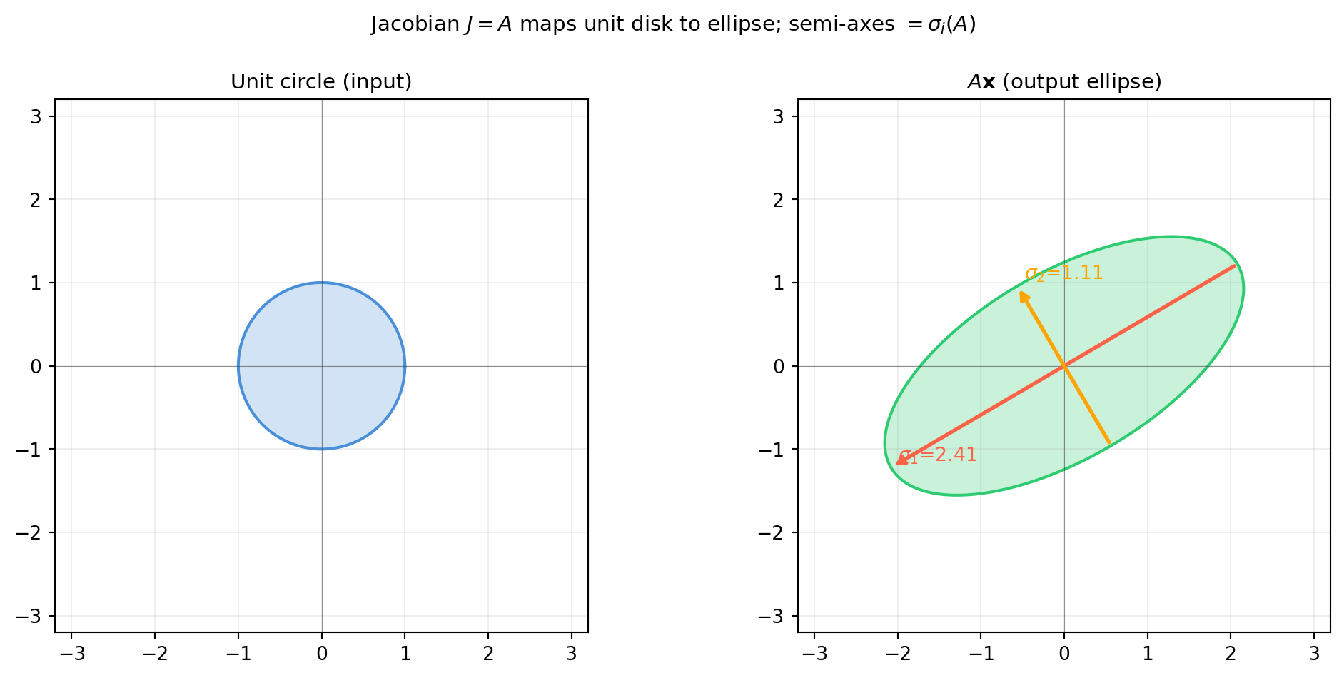
# A linear map with clear stretching and rotation
A = np.array([[2.0, 0.8],
              [0.4, 1.5]])              # shape (2, 2)

ellipse = A @ circle                   # shape (2, 500)  -- Jacobian = A

# SVD to find semi-axes
U, s, Vt = np.linalg.svd(A)           # s shape (2,)
V = Vt.T                               # columns = right singular vectors

fig, axes = plt.subplots(1, 2, figsize=(11, 5))

for ax, pts, title, col in zip(
    axes,
    [circle, ellipse],
    ['Unit circle (input)', r'$A\mathbf{x}$ (output ellipse)'],
    ['#4a90d9', '#2ecc71']
):
    ax.fill(pts[0], pts[1], color=col, alpha=0.25)
    ax.plot(pts[0], pts[1], color=col, lw=1.5)
    ax.axhline(0, color='#333333', lw=0.4, alpha=0.5)
    ax.axvline(0, color='#333333', lw=0.4, alpha=0.5)
    ax.set_aspect('equal')
    ax.set_title(title, fontsize=11)
    ax.grid(alpha=0.2)

# Annotate semi-axes on ellipse panel
ax = axes[1]
for i, (si, col_a, lbl) in enumerate(
    zip(s, ['tomato', 'orange'], [r'$\sigma_1$', r'$\sigma_2$'])
):
    v = U[:, i]                        # left singular vector (output direction)
    ax.annotate('', xy=si*v, xytext=-si*v,
                arrowprops=dict(arrowstyle='->', color=col_a, lw=2))
    ax.text(*(si*v + np.array([0.08, 0.08])), f'{lbl}={si:.2f}',
            fontsize=10, color=col_a)

axes[0].set_xlim(-3.2, 3.2); axes[0].set_ylim(-3.2, 3.2)
axes[1].set_xlim(-3.2, 3.2); axes[1].set_ylim(-3.2, 3.2)
fig.suptitle(r'Jacobian $J=A$ maps unit disk to ellipse; semi-axes $=\sigma_i(A)$',
             fontsize=11)
fig.tight_layout()
plt.savefig('ch21-matrix-calculus/fig-jacobian-ellipse.png', dpi=150, bbox_inches='tight')
plt.show()
print(f"Singular values of A: sigma_1={s[0]:.4f}, sigma_2={s[1]:.4f}")
print(f"det(A) = {np.linalg.det(A):.4f}  (= sigma_1 * sigma_2 = area scale factor)")

Singular values of A: sigma_1=2.4114, sigma_2=1.1114
det(A) = 2.6800  (= sigma_1 * sigma_2 = area scale factor)

The unit circle stretches into an ellipse whose semi-axis lengths are the singular values of \(A\) (= the Jacobian). The determinant \(\det(A)=\sigma_1\sigma_2\) measures the local area scaling factor – how much a small patch of input space expands or contracts under \(\mathbf{f}\).

---

21.3.5 Numerical Verification

import numpy as np

rng = np.random.default_rng(2131)
n, m = 3, 4

# Test function: f_i(x) = sin(a_i^T x)  -- nonlinear
A = rng.standard_normal((m, n))     # shape (4, 3)
x0 = rng.standard_normal(n)        # shape (3,)

def f_vec(x):
    return np.sin(A @ x)            # shape (4,)

# Exact Jacobian: J_ij = d/dx_j sin(sum_k A_ik x_k) = cos(A_i . x) * A_ij
J_exact = np.diag(np.cos(A @ x0)) @ A   # shape (4, 3)

# Finite-difference Jacobian
h = 1e-5
J_fd = np.zeros((m, n))             # shape (4, 3)
for j in range(n):
    e = np.zeros(n); e[j] = h
    J_fd[:, j] = (f_vec(x0 + e) - f_vec(x0 - e)) / (2 * h)

print("Jacobian shape:", J_exact.shape)
print("Max |exact - FD|:", np.max(np.abs(J_exact - J_fd)))

# Verify local linearization
dxs = rng.standard_normal(n) * 0.01    # small perturbation, shape (3,)
df_linear = J_exact @ dxs              # shape (4,)
df_exact  = f_vec(x0 + dxs) - f_vec(x0)  # shape (4,)
print(f"Linearization error (||dx||={np.linalg.norm(dxs):.4f}):",
      np.max(np.abs(df_exact - df_linear)))

Jacobian shape: (4, 3)
Max |exact - FD|: 2.993649772520257e-10
Linearization error (||dx||=0.0178): 0.000182810299599696

The linearization error is \(O(\|\delta\mathbf{x}\|^2)\approx 10^{-6}\) for \(\|\delta\mathbf{x}\|\approx 0.01\) – confirming the quadratic falloff of the Taylor approximation error.

---

21.3.6 Exercises

21.3.1 Write out the Jacobian of \(\mathbf{f}(\mathbf{x})=A\mathbf{x}+\mathbf{b}\) (affine map) for \(A\in\mathbb{R}^{m\times n}\). Why does the constant vector \(\mathbf{b}\) not appear in the Jacobian?

21.3.2 Compute the Jacobian of the element-wise ReLU: \(f_i(x) = \max(0, x_i)\). Is the Jacobian always well-defined? What happens at \(x_i=0\)?

21.3.3 Let \(\mathbf{f}(\mathbf{x})=\mathbf{x}/\|\mathbf{x}\|\) (unit normalization, \(\mathbb{R}^n\to\mathbb{R}^n\)). Show that \(J=\frac{1}{\|\mathbf{x}\|}(I - \hat{\mathbf{x}}\hat{\mathbf{x}}^T)\) where \(\hat{\mathbf{x}}=\mathbf{x}/\|\mathbf{x}\|\). Interpret the rank of \(J\).

21.3.4 For a differentiable map \(\mathbf{f}:\mathbb{R}^n\to\mathbb{R}^m\) and \(\mathbf{g}:\mathbb{R}^m\to\mathbb{R}^p\), the Jacobian of \(\mathbf{h}=\mathbf{g}\circ\mathbf{f}\) is \(J_h = J_g J_f\) (matrix chain rule). Verify dimensionally that \(J_h\in\mathbb{R}^{p\times n}\).

21.3.5 The local linearization says \(\mathbf{f}(\mathbf{x}_0+\delta\mathbf{x})\approx\mathbf{f}(\mathbf{x}_0)+J\delta\mathbf{x}\). For a linear function \(\mathbf{f}(\mathbf{x})=A\mathbf{x}\), is this approximation exact? Why?

21.4 Scalar-by-Matrix: Weight Gradients

In neural networks the parameters are matrices \(W\in\mathbb{R}^{m\times n}\). Training requires computing \(\partial L/\partial W\) – the derivative of a scalar loss with respect to every element of \(W\). This section develops the key identities, beginning with an honest account of what \(\partial(W\mathbf{x})/\partial W\) actually is.

---

21.4.1 The Tensor Elephant in the Room

Consider the simplest case: \(\mathbf{y}=W\mathbf{x}\) where \(W\in\mathbb{R}^{m\times n}\), \(\mathbf{x}\in\mathbb{R}^n\), and \(\mathbf{y}\in\mathbb{R}^m\). The quantity \(\partial\mathbf{y}/\partial W\) is the derivative of an \(m\)-vector with respect to an \(m\times n\) matrix. Storing every partial derivative \(\partial y_i/\partial W_{jk}\) requires an \(m\times m\times n\) array – a third-order tensor.

That tensor is rarely written out in full. Instead, training uses the scalar loss \(L:\mathbb{R}\to\mathbb{R}\), and the quantity we actually need is \(\partial L/\partial W\) – the derivative of a scalar with respect to a matrix. This is a genuine \(m\times n\) matrix (same shape as \(W\)), not a tensor.

---

21.4.2 The Backpropagation Shortcut: \(\partial L/\partial W = \boldsymbol{\delta}\mathbf{x}^T\)

Suppose \(\mathbf{y}=W\mathbf{x}\) and \(L=L(\mathbf{y})\). Define the error signal \(\boldsymbol{\delta}=\partial L/\partial\mathbf{y}\in\mathbb{R}^m\) (a column vector; denominator layout from §21.1). By the chain rule applied element-wise:

\[\frac{\partial L}{\partial W_{ij}} = \sum_k \frac{\partial L}{\partial y_k}\frac{\partial y_k}{\partial W_{ij}} = \sum_k \delta_k \cdot [x_j \text{ if } k=i, \text{ else } 0] = \delta_i x_j.\]

Assembling all \((i,j)\) pairs:

\[\boxed{\frac{\partial L}{\partial W} = \boldsymbol{\delta}\mathbf{x}^T.}\]

This is an outer product of the upstream error \(\boldsymbol{\delta}\) and the input \(\mathbf{x}\). The result has shape \(m\times n\) = same as \(W\). This identity is the heart of every neural network gradient update.

---

21.4.3 Three More Matrix-Derivative Identities

Identity: Trace form

\[\frac{\partial}{\partial W}\text{tr}(WA) = A^T.\]

Derivation. \(\text{tr}(WA)=\sum_{i,j}W_{ij}A_{ji}\), so \(\partial/\partial W_{ij}[\text{tr}(WA)] = A_{ji}=(A^T)_{ij}\). Assembling: \(\partial\text{tr}(WA)/\partial W = A^T\).

Identity: Symmetric quadratic form

\[\frac{\partial}{\partial W}(\mathbf{x}^TW\mathbf{x}) = \mathbf{x}\mathbf{x}^T.\]

Derivation. \(\mathbf{x}^TW\mathbf{x}=\sum_{i,j}x_iW_{ij}x_j\), so \(\partial/\partial W_{ij}[\mathbf{x}^TW\mathbf{x}] = x_ix_j=(\mathbf{x}\mathbf{x}^T)_{ij}\).

Identity: Frobenius norm

\[\frac{\partial}{\partial W}\|W\|_F^2 = 2W.\]

Derivation. \(\|W\|_F^2=\sum_{i,j}W_{ij}^2\), so \(\partial/\partial W_{ij}[\sum_{k,l}W_{kl}^2]=2W_{ij}\). This identity appears in nuclear-norm and weight-decay regularization.

---

21.4.4 Summary Table

Expression	\(\partial/\partial W\)	Shape
\(\text{tr}(WA)\)	\(A^T\)	\(m\times n\)
\(\mathbf{x}^TW\mathbf{x}\) (\(W\) square)	\(\mathbf{x}\mathbf{x}^T\)	\(n\times n\)
\(\|W\|_F^2\)	\(2W\)	\(m\times n\)
\(L(\mathbf{y}=W\mathbf{x})\)	\(\boldsymbol{\delta}\mathbf{x}^T\), \(\boldsymbol{\delta}=\nabla_\mathbf{y}L\)	\(m\times n\)

---

21.4.5 Numerical Verification

import numpy as np

rng = np.random.default_rng(2141)
m, n = 3, 4
W = rng.standard_normal((m, n))    # shape (3, 4)
A = rng.standard_normal((n, m))    # shape (4, 3)
x = rng.standard_normal(n)         # shape (4,)
x_sq = rng.standard_normal(n)      # shape (4,) for the quadratic form test (W square)
Wsq = rng.standard_normal((n, n))  # shape (4, 4)

def fd_mat_grad(f_scalar, W, h=1e-5):
    """Finite-difference gradient w.r.t. matrix W."""
    G = np.zeros_like(W)
    for i in range(W.shape[0]):
        for j in range(W.shape[1]):
            Wp = W.copy(); Wp[i,j] += h
            Wm = W.copy(); Wm[i,j] -= h
            G[i,j] = (f_scalar(Wp) - f_scalar(Wm)) / (2*h)
    return G

# Identity: d tr(WA)/dW = A^T
g_exact1 = A.T                                     # shape (3, 4)
g_fd1    = fd_mat_grad(lambda W: np.trace(W @ A), W)
print(f"d tr(WA)/dW = A^T      max|error| = {np.max(np.abs(g_exact1 - g_fd1)):.2e}")

# Identity: d(x^T W x)/dW = x x^T  (W square)
g_exact2 = np.outer(x_sq, x_sq)                    # shape (4, 4)
g_fd2    = fd_mat_grad(lambda W: float(x_sq @ W @ x_sq), Wsq)
print(f"d(x^T W x)/dW = x x^T max|error| = {np.max(np.abs(g_exact2 - g_fd2)):.2e}")

# Identity: d ||W||_F^2/dW = 2W
g_exact3 = 2 * W                                    # shape (3, 4)
g_fd3    = fd_mat_grad(lambda W: float(np.sum(W**2)), W)
print(f"d||W||_F^2/dW = 2W     max|error| = {np.max(np.abs(g_exact3 - g_fd3)):.2e}")

# Identity: dL/dW = delta x^T  (L = 0.5 ||Wx - t||^2)
t = rng.standard_normal(m)                          # shape (3,) target
y = W @ x                                           # shape (3,)
delta = y - t                                       # shape (3,) -- gradient of 0.5||y-t||^2
g_exact4 = np.outer(delta, x)                       # shape (3, 4)
g_fd4    = fd_mat_grad(
    lambda W: 0.5 * float((W @ x - t) @ (W @ x - t)), W)
print(f"dL/dW = delta x^T       max|error| = {np.max(np.abs(g_exact4 - g_fd4)):.2e}")

d tr(WA)/dW = A^T      max|error| = 2.36e-11
d(x^T W x)/dW = x x^T max|error| = 1.07e-11
d||W||_F^2/dW = 2W     max|error| = 9.96e-11
dL/dW = delta x^T       max|error| = 2.73e-11

All four identities are verified to near machine precision.

---

21.4.6 Exercises

21.4.1 The identity \(\partial L/\partial W = \boldsymbol{\delta}\mathbf{x}^T\) is an outer product. What is its rank? When could it be full rank, and when is it rank-1?

21.4.2 Derive \(\partial\text{tr}(W^T A)/\partial W\) where \(A\) is a fixed matrix. (Hint: \(\text{tr}(W^T A)=\text{tr}(A^T W)\); use the trace identity with appropriate substitution.)

21.4.3 Show that \(\partial\|W\mathbf{x}-\mathbf{b}\|^2/\partial W = 2(W\mathbf{x}-\mathbf{b})\mathbf{x}^T\). (Hint: write the loss as \(\text{tr}[(W\mathbf{x}-\mathbf{b})(W\mathbf{x}-\mathbf{b})^T]\), or use the backprop shortcut with \(\boldsymbol{\delta}=2(W\mathbf{x}-\mathbf{b})\).)

21.4.4 In weight-decay regularization, the total loss is \(L_\text{total}=L_\text{data}+(\lambda/2)\|W\|_F^2\). What is \(\partial L_\text{total}/\partial W\)? If you are using gradient descent, how does the weight-decay term modify the parameter update?

21.4.5 Why is \(\partial\mathbf{y}/\partial W\) (for \(\mathbf{y}=W\mathbf{x}\)) a 3-index tensor while \(\partial L/\partial W\) is a matrix? Explain what additional information must be provided to collapse the tensor to a matrix.

21.5 The Chain Rule in Matrix Form

The chain rule for scalar functions says \((g\circ f)'(x)=g'(f(x))\cdot f'(x)\). In higher dimensions each prime becomes a Jacobian, and the product becomes a matrix multiplication. This section traces that idea through a complete neural network layer.

---

21.5.1 The Matrix Chain Rule

Let \(\mathbf{f}:\mathbb{R}^n\to\mathbb{R}^m\) and \(\mathbf{g}:\mathbb{R}^m\to\mathbb{R}^p\). Define \(\mathbf{h}=\mathbf{g}\circ\mathbf{f}\), so \(\mathbf{h}:\mathbb{R}^n\to\mathbb{R}^p\). The Jacobian of \(\mathbf{h}\) is the product of the individual Jacobians:

\[J_h = J_g\,J_f \;\in\;\mathbb{R}^{p\times n},\]

where \(J_f\in\mathbb{R}^{m\times n}\) and \(J_g\in\mathbb{R}^{p\times m}\). Shape check: \((p\times m)(m\times n)=(p\times n)\) – consistent.

For a scalar terminal loss \(L\) (\(p=1\)), the gradient through the composition is

\[\frac{\partial L}{\partial\mathbf{x}} = J_f^T\,\frac{\partial L}{\partial\mathbf{f}} \;\in\;\mathbb{R}^n,\]

where \(\partial L/\partial\mathbf{f}\in\mathbb{R}^m\) is the upstream gradient (denominator layout: a column vector). Each layer in a neural network propagates gradients backward through this rule.

---

21.5.2 End-to-End: A Single Linear Layer

The simplest complete example is a linear layer followed by a squared loss.

Forward pass:

\[\mathbf{y} = W\mathbf{x}+\mathbf{b},\qquad L = \frac{1}{2}\|\mathbf{y}-\mathbf{t}\|^2,\]

where \(W\in\mathbb{R}^{m\times n}\), \(\mathbf{x}\in\mathbb{R}^n\), \(\mathbf{b}\in\mathbb{R}^m\), and \(\mathbf{t}\in\mathbb{R}^m\) is the target.

Backward pass:

Step 1 – gradient of \(L\) with respect to \(\mathbf{y}\):

\[\boldsymbol{\delta} = \frac{\partial L}{\partial\mathbf{y}} = \mathbf{y}-\mathbf{t} \;\in\;\mathbb{R}^m.\]

Step 2 – gradient with respect to \(W\) (from §21.4):

\[\frac{\partial L}{\partial W} = \boldsymbol{\delta}\mathbf{x}^T \;\in\;\mathbb{R}^{m\times n}.\]

Step 3 – gradient with respect to \(\mathbf{b}\) (since \(\partial\mathbf{y}/\partial\mathbf{b}=I\)):

\[\frac{\partial L}{\partial\mathbf{b}} = \boldsymbol{\delta} \;\in\;\mathbb{R}^m.\]

Step 4 – gradient with respect to \(\mathbf{x}\) (to propagate to earlier layers; Jacobian of \(W\mathbf{x}\) w.r.t. \(\mathbf{x}\) is \(W\), so we use \(J^T\boldsymbol{\delta}\)):

\[\frac{\partial L}{\partial\mathbf{x}} = W^T\boldsymbol{\delta} \;\in\;\mathbb{R}^n.\]

These four equations constitute one complete backpropagation pass through a linear layer. Notice the pattern: going backward, matrices appear transposed.

---

21.5.3 Code: Forward and Backward with Finite-Difference Verification

import numpy as np

rng = np.random.default_rng(2151)
m, n = 4, 3

W = rng.standard_normal((m, n))    # shape (4, 3)
b = rng.standard_normal(m)         # shape (4,)
x = rng.standard_normal(n)         # shape (3,)
t = rng.standard_normal(m)         # shape (4,) target

# --- Forward pass ---
y = W @ x + b                      # shape (4,)
L = 0.5 * float((y - t) @ (y - t))

# --- Backward pass ---
delta = y - t                      # shape (4,)   dL/dy
dL_dW = np.outer(delta, x)         # shape (4, 3) dL/dW = delta x^T
dL_db = delta.copy()               # shape (4,)   dL/db = delta
dL_dx = W.T @ delta                # shape (3,)   dL/dx = W^T delta

print(f"Forward: L = {L:.6f}")
print(f"dL/dW shape: {dL_dW.shape}")
print(f"dL/db shape: {dL_db.shape}")
print(f"dL/dx shape: {dL_dx.shape}")

# --- Finite-difference verification ---
h = 1e-5

def L_from_W(W_):
    y_ = W_ @ x + b
    return 0.5 * float((y_ - t) @ (y_ - t))

def L_from_b(b_):
    y_ = W @ x + b_
    return 0.5 * float((y_ - t) @ (y_ - t))

def L_from_x(x_):
    y_ = W @ x_ + b
    return 0.5 * float((y_ - t) @ (y_ - t))

# dL/dW by FD
dW_fd = np.zeros((m, n))
for i in range(m):
    for j in range(n):
        Wp = W.copy(); Wp[i,j] += h
        Wm = W.copy(); Wm[i,j] -= h
        dW_fd[i,j] = (L_from_W(Wp) - L_from_W(Wm)) / (2*h)

# dL/db by FD
db_fd = np.zeros(m)
for i in range(m):
    ep = np.zeros(m); ep[i] = h
    db_fd[i] = (L_from_b(b + ep) - L_from_b(b - ep)) / (2*h)

# dL/dx by FD
dx_fd = np.zeros(n)
for i in range(n):
    ep = np.zeros(n); ep[i] = h
    dx_fd[i] = (L_from_x(x + ep) - L_from_x(x - ep)) / (2*h)

print(f"\ndL/dW  max|exact - FD| = {np.max(np.abs(dL_dW - dW_fd)):.2e}")
print(f"dL/db  max|exact - FD| = {np.max(np.abs(dL_db - db_fd)):.2e}")
print(f"dL/dx  max|exact - FD| = {np.max(np.abs(dL_dx - dx_fd)):.2e}")

Forward: L = 3.626794
dL/dW shape: (4, 3)
dL/db shape: (4,)
dL/dx shape: (3,)

dL/dW  max|exact - FD| = 1.26e-11
dL/db  max|exact - FD| = 2.44e-11
dL/dx  max|exact - FD| = 3.38e-11

All three gradients match finite differences to near machine precision, confirming the backward-pass equations.

---

21.5.4 Stacking Layers: Computational Graph

For a two-layer network \(L = \ell(\mathbf{y}_2),\; \mathbf{y}_2 = W_2\phi(\mathbf{y}_1),\; \mathbf{y}_1 = W_1\mathbf{x}+\mathbf{b}_1\) (where \(\phi\) is element-wise), the chain rule applies sequentially:

\[\frac{\partial L}{\partial W_1} = \boldsymbol{\delta}_1\mathbf{x}^T,\qquad \boldsymbol{\delta}_1 = \text{diag}(\phi'(\mathbf{y}_1))\,W_2^T\boldsymbol{\delta}_2,\qquad \boldsymbol{\delta}_2 = \frac{\partial\ell}{\partial\mathbf{y}_2}.\]

Each layer’s error signal \(\boldsymbol{\delta}\) is the upstream error transformed by the transpose of the weight matrix and element-wise multiplied by the activation derivative – precisely what automatic differentiation frameworks compute.

---

21.5.5 Exercises

21.5.1 In the single linear layer example, derive \(\partial L/\partial\mathbf{b}=\boldsymbol{\delta}\) from first principles using the chain rule (not by inspection). What is the Jacobian of \(\mathbf{y}=W\mathbf{x}+\mathbf{b}\) with respect to \(\mathbf{b}\)?

21.5.2 Let \(L=\frac{1}{2}\|\mathbf{y}-\mathbf{t}\|^2\) and \(\mathbf{y}=\sigma(W\mathbf{x}+\mathbf{b})\) where \(\sigma\) is applied element-wise. Using the chain rule, derive \(\partial L/\partial W\). Compare to the linear-layer case – what is the only difference?

21.5.3 Show that the gradient \(\partial L/\partial\mathbf{x}=W^T\boldsymbol{\delta}\) is consistent with the matrix chain rule \(J_f^T(\partial L/\partial\mathbf{f})\) where \(\mathbf{f}(\mathbf{x})=W\mathbf{x}+\mathbf{b}\).

21.5.4 When would you use finite differences (as in the verification code above) in practice? What are the downsides compared to automatic differentiation?

21.5.5 Consider a loss \(L = \frac{1}{N}\sum_{k=1}^N \frac{1}{2}\|W\mathbf{x}_k+\mathbf{b}-\mathbf{t}_k\|^2\) over a batch of \(N\) examples. Show that \(\partial L/\partial W = \frac{1}{N}\sum_k\boldsymbol{\delta}_k\mathbf{x}_k^T\). In matrix form, if \(\Delta = [\boldsymbol{\delta}_1,\ldots,\boldsymbol{\delta}_N]\in\mathbb{R}^{m\times N}\) and \(X = [\mathbf{x}_1,\ldots,\mathbf{x}_N]\in\mathbb{R}^{n\times N}\), write this as a single matrix expression.

21.6 The Hessian Matrix

The gradient \(\nabla f\) tells you how steeply the loss climbs in each direction. The Hessian \(H\) encodes the curvature: how quickly the gradient itself changes, and therefore how quickly gradient descent will converge near a critical point.

---

21.6.1 Definition

Let \(f:\mathbb{R}^n\to\mathbb{R}\) be twice differentiable. The Hessian is the \(n\times n\) matrix of second-order partial derivatives:

\[H_{ij} = \frac{\partial^2 f}{\partial x_i\,\partial x_j}.\]

Equivalently, \(H = \nabla^2 f\) (the gradient of the gradient), or

\[H = \frac{\partial}{\partial\mathbf{x}}(\nabla_\mathbf{x}f)^T = \frac{\partial^2 f}{\partial\mathbf{x}\partial\mathbf{x}^T}.\]

Symmetry. By Schwarz’s theorem (equality of mixed partials under continuity), \(H_{ij}=H_{ji}\) for all \(i,j\). The Hessian is always symmetric: \(H=H^T\). Since it is real and symmetric, all its eigenvalues are real (§13.4).

---

21.6.2 What the Eigenvalues Tell You

Applying the second-order Taylor expansion at a critical point \(\mathbf{x}_0\) where \(\nabla f(\mathbf{x}_0)=\mathbf{0}\):

\[f(\mathbf{x}_0+\delta\mathbf{x}) \approx f(\mathbf{x}_0) + \frac{1}{2}\delta\mathbf{x}^T H\,\delta\mathbf{x}.\]

The sign of the quadratic form \(\delta\mathbf{x}^T H\,\delta\mathbf{x}\) determines the nature of the critical point:

Hessian eigenvalues	Classification
All \(\lambda_i > 0\) (\(H\) positive definite)	Local minimum – every direction curves up
All \(\lambda_i < 0\) (\(H\) negative definite)	Local maximum – every direction curves down
Mixed signs	Saddle point – some directions up, some down
Some \(\lambda_i = 0\)	Inconclusive (degenerate case)

Saddle points are ubiquitous in deep learning loss surfaces: a network with many parameters nearly always has directions of negative curvature at any interior critical point. Gradient descent slows near saddle points because the gradient is small in those flat directions, but does eventually escape due to asymmetric curvature.

---

21.6.3 Example: Hessians of Common Loss Functions

Squared loss \(f(\mathbf{x})=\|A\mathbf{x}-\mathbf{b}\|^2\): \(\nabla f=2A^T(A\mathbf{x}-\mathbf{b})\), so \(H=\nabla(\nabla f)^T=2A^TA\). Since \(A^TA\) is always positive semidefinite (PSD), the squared loss is convex – there are no saddle points, only a (possibly non-unique) global minimum.

Quadratic form \(f(\mathbf{x})=\mathbf{x}^TA\mathbf{x}\) with symmetric \(A\): \(H=2A\).

Rosenbrock (non-convex) \(f(x_1,x_2)=100(x_2-x_1^2)^2+(1-x_1)^2\):

\[H = \begin{pmatrix}1200x_1^2-400x_2+2 & -400x_1 \\ -400x_1 & 200\end{pmatrix}.\]

At the minimum \((1,1)\): \(H=\begin{pmatrix}802&-400\\-400&200\end{pmatrix}\), which is positive definite (both eigenvalues \(>0\)).

---

21.6.4 Newton’s Method

Newton’s method exploits the Hessian to take curvature-aware steps:

\[\mathbf{x}_{k+1} = \mathbf{x}_k - H^{-1}\nabla f(\mathbf{x}_k).\]

The step \(-H^{-1}\nabla f\) solves for the minimum of the local quadratic approximation. Compared to gradient descent (step \(-\alpha\nabla f\)):

• Gradient descent step size \(\alpha\) must be tuned; convergence is linear.
• Newton’s method automatically accounts for curvature; convergence is quadratic near the minimum.

The cost: computing \(H\) requires \(O(n^2)\) memory and \(O(n^3)\) to invert. For large neural networks (\(n\sim10^8\) parameters) exact Newton’s method is infeasible. Practical alternatives include quasi-Newton methods (L-BFGS, which approximates \(H^{-1}\) without forming \(H\)) and Gauss-Newton.

---

21.6.5 Gauss-Newton Approximation

For a least-squares loss \(L(\mathbf{x})=\frac{1}{2}\|\mathbf{r}(\mathbf{x})\|^2\) with residual vector \(\mathbf{r}:\mathbb{R}^n\to\mathbb{R}^m\):

\[\nabla L = J_r^T\mathbf{r}, \qquad H = J_r^T J_r + \sum_i r_i H_i \approx J_r^T J_r,\]

where \(H_i\) is the Hessian of the \(i\)-th residual. Dropping the second-order term \(\sum r_i H_i\) (small near the solution) gives the Gauss-Newton approximation \(H\approx J_r^TJ_r\). This matrix is always positive semidefinite – no saddle points, and no need to compute second derivatives. It is the foundation of the Levenberg-Marquardt optimizer used in ICP, bundle adjustment, and graph-SLAM (Ch 22, Ch 24).

---

21.6.6 Visualization: Bowl vs. Saddle

import numpy as np
import matplotlib.pyplot as plt

x1v = np.linspace(-2.5, 2.5, 200)    # shape (200,)
x2v = np.linspace(-2.5, 2.5, 200)    # shape (200,)
X1, X2 = np.meshgrid(x1v, x2v)       # each shape (200, 200)

# Bowl: f = x1^2 + 2*x2^2 (PD Hessian diag(2, 4))
F_bowl   = X1**2 + 2*X2**2
# Saddle: f = x1^2 - x2^2 (indefinite Hessian diag(2, -2))
F_saddle = X1**2 - X2**2

fig, axes = plt.subplots(1, 2, figsize=(12, 5))

titles = [
    r'Bowl: $f=x_1^2+2x_2^2$ (PD Hessian -- minimum)',
    r'Saddle: $f=x_1^2-x_2^2$ (indefinite -- saddle)'
]
Fs = [F_bowl, F_saddle]

for ax, F, title in zip(axes, Fs, titles):
    cf = ax.contourf(X1, X2, F, levels=20, cmap='Blues', alpha=0.55)
    plt.colorbar(cf, ax=ax, shrink=0.8)
    ax.contour(X1, X2, F, levels=10, colors='#4a90d9', linewidths=0.6, alpha=0.7)
    ax.axhline(0, color='#333333', lw=0.4, alpha=0.5)
    ax.axvline(0, color='#333333', lw=0.4, alpha=0.5)
    ax.set_xlabel(r'$x_1$', fontsize=11)
    ax.set_ylabel(r'$x_2$', fontsize=11)
    ax.set_title(title, fontsize=10)
    ax.set_aspect('equal')
    ax.grid(alpha=0.2)
    ax.plot(0, 0, 'o', color='tomato', ms=7, zorder=5, label='critical point')
    ax.legend(fontsize=9)

fig.tight_layout()
plt.savefig('ch21-matrix-calculus/fig-hessian-bowl-saddle.png',
            dpi=150, bbox_inches='tight')
plt.show()

For the bowl, the Hessian \(H=\text{diag}(2,4)\) has all positive eigenvalues \((2,4)\) – every direction curves upward, and the critical point at the origin is a minimum. For the saddle, \(H=\text{diag}(2,-2)\) has mixed signs – the \(x_1\) direction curves up but the \(x_2\) direction curves down, so the origin is neither a minimum nor a maximum.

---

21.6.7 Numerical Hessian via Finite Differences

import numpy as np

def hessian_fd(f, x, h=1e-4):
    """Finite-difference Hessian via central differences."""
    n = len(x)
    H = np.zeros((n, n))             # shape (n, n)
    for i in range(n):
        for j in range(i, n):
            ei = np.zeros(n); ei[i] = h
            ej = np.zeros(n); ej[j] = h
            H[i, j] = (f(x+ei+ej) - f(x+ei-ej)
                       - f(x-ei+ej) + f(x-ei-ej)) / (4*h**2)
            H[j, i] = H[i, j]       # symmetry
    return H

# f = ||Ax - b||^2, exact Hessian = 2 A^T A
rng = np.random.default_rng(2161)
m, n = 5, 3
A = rng.standard_normal((m, n))     # shape (5, 3)
b = rng.standard_normal(m)          # shape (5,)
x = rng.standard_normal(n)          # shape (3,)

H_exact = 2 * A.T @ A               # shape (3, 3)
H_fd    = hessian_fd(lambda x: float((A@x-b) @ (A@x-b)), x)

print("Exact Hessian:\n", np.round(H_exact, 4))
print("\nFD Hessian:\n",   np.round(H_fd, 4))
print("\nMax |error|:", np.max(np.abs(H_exact - H_fd)))
print("Hessian eigenvalues:", np.round(np.linalg.eigvalsh(H_exact), 4),
      " -- all >= 0 (PSD): convex loss")

Exact Hessian:
 [[ 2.5972  1.3837  0.4788]
 [ 1.3837  3.1051 -1.8519]
 [ 0.4788 -1.8519  5.7194]]

FD Hessian:
 [[ 2.5972  1.3837  0.4788]
 [ 1.3837  3.1051 -1.8519]
 [ 0.4788 -1.8519  5.7194]]

Max |error|: 1.3946681143295336e-08
Hessian eigenvalues: [0.9017 3.8287 6.6913]  -- all >= 0 (PSD): convex loss

---

21.6.8 Exercises

21.6.1 Compute the Hessian of \(f(\mathbf{x})=\mathbf{x}^T\Sigma^{-1}\mathbf{x}\) where \(\Sigma\) is a symmetric PD matrix. Is the Hessian positive definite? What does this imply about the shape of the Mahalanobis distance landscape?

21.6.2 For the saddle function \(f(x_1,x_2)=x_1^2-x_2^2\), verify by hand that the Hessian is indefinite (mixed eigenvalue signs). In which direction does the function decrease from the origin?

21.6.3 Why does Newton’s method converge quadratically near a minimum but may diverge or oscillate far from it? What modification (e.g., line search or damping) is typically added in practice?

21.6.4 For the Gauss-Newton approximation \(H\approx J_r^TJ_r\), explain why this matrix is always positive semidefinite. Under what condition is it positive definite (and hence the Newton system has a unique solution)?

21.6.5 The condition number \(\kappa(H)=\lambda_{\max}/\lambda_{\min}\) controls how quickly gradient descent converges: the number of iterations scales as \(O(\kappa(H)\log(1/\varepsilon))\). Given the Hessian in the numerical example above, compute \(\kappa(H)\) and predict which direction gradient descent converges slowest.

21.7 Key Identity Reference Table

The table below collects the identities used most often in ML, CV, and robotics. All derivatives follow denominator layout (column-vector gradients; Jacobian \(J_{ij}=\partial f_i/\partial x_j\in\mathbb{R}^{m\times n}\)) as established in §21.1. Derivation sketches for every identity are in Appendix D.

---

21.7.1 Category 1: Scalar-by-Vector (Gradients)

Expression \(f(\mathbf{x})\)	\(\nabla_\mathbf{x}f\)	Conditions
\(\mathbf{a}^T\mathbf{x}\)	\(\mathbf{a}\)
\(\mathbf{x}^T\mathbf{a}\)	\(\mathbf{a}\)	same as above
\(\mathbf{x}^TA\mathbf{x}\)	\((A+A^T)\mathbf{x}\)
\(\mathbf{x}^TA\mathbf{x}\)	\(2A\mathbf{x}\)	\(A\) symmetric
\(\|A\mathbf{x}-\mathbf{b}\|^2\)	\(2A^T(A\mathbf{x}-\mathbf{b})\)
\(\|\mathbf{x}\|^2\)	\(2\mathbf{x}\)
\((\mathbf{x}-\boldsymbol{\mu})^T\Sigma^{-1}(\mathbf{x}-\boldsymbol{\mu})\)	\(2\Sigma^{-1}(\mathbf{x}-\boldsymbol{\mu})\)	\(\Sigma\) symmetric PD

---

21.7.2 Category 2: Scalar-by-Matrix (Weight Gradients)

Expression \(f(W)\)	\(\partial f/\partial W\)	Conditions
\(\text{tr}(WA)\)	\(A^T\)
\(\text{tr}(AW)\)	\(A^T\)	same as above
\(\text{tr}(W^TA)\)	\(A\)
\(\text{tr}(AWBW^T)\)	\(A^TW B^T+AWB\)
\(\mathbf{a}^TW\mathbf{b}\)	\(\mathbf{a}\mathbf{b}^T\)
\(\mathbf{x}^TW\mathbf{x}\)	\(\mathbf{x}\mathbf{x}^T\)	\(W\) square
\(\|W\|_F^2\)	\(2W\)
\(L(W\mathbf{x}+\mathbf{b})\)	\((\nabla_\mathbf{y}L)\mathbf{x}^T\)	\(\mathbf{y}=W\mathbf{x}+\mathbf{b}\)

---

21.7.3 Category 3: Vector-by-Vector (Jacobians)

Map \(\mathbf{f}(\mathbf{x})\)	Jacobian \(J=\partial\mathbf{f}/\partial\mathbf{x}\)	Shape
\(A\mathbf{x}+\mathbf{b}\)	\(A\)	\(m\times n\)
\(\mathbf{x}^{\odot2}\) (element-wise square)	\(2\,\text{diag}(\mathbf{x})\)	\(n\times n\)
\(\sigma(\mathbf{x})\) (element-wise sigmoid)	\(\text{diag}(\sigma'(\mathbf{x}))\)	\(n\times n\)
\(\phi(\mathbf{x})\) (any element-wise)	\(\text{diag}(\phi'(\mathbf{x}))\)	\(n\times n\)
\(\mathbf{x}/\|\mathbf{x}\|\)	\((I-\hat{\mathbf{x}}\hat{\mathbf{x}}^T)/\|\mathbf{x}\|\)	\(n\times n\)
\(A\mathbf{f}(\mathbf{x})\)	\(A\,J_f\)	\(m\times n\)

---

21.7.4 Category 4: Hessians

Expression \(f(\mathbf{x})\)	Hessian \(H=\nabla^2 f\)	Type
\(\mathbf{a}^T\mathbf{x}\)	\(0\)	zero
\(\mathbf{x}^TA\mathbf{x}\)	\(A+A^T\)	symmetric
\(\mathbf{x}^TA\mathbf{x}\)	\(2A\)	symmetric; \(A\) symmetric
\(\|A\mathbf{x}-\mathbf{b}\|^2\)	\(2A^TA\)	PSD
\(\|\mathbf{r}(\mathbf{x})\|^2\) (nonlinear \(\mathbf{r}\))	\(\approx 2J_r^TJ_r\) (Gauss-Newton)	PSD approximation
\(f(\mathbf{x})=g(A\mathbf{x})\)	\(A^T H_g A\)	inherits definiteness of \(H_g\)

---

21.7.5 Chain Rule Summary

Scenario	Formula
Scalar \(L\) via \(\mathbf{f}:\mathbb{R}^n\to\mathbb{R}^m\)	\(\nabla_\mathbf{x}L = J_f^T\,\nabla_\mathbf{f}L\)
Vector \(\mathbf{h}=\mathbf{g}\circ\mathbf{f}\)	\(J_h = J_g\,J_f\)
Linear layer backward	\(\partial L/\partial W=\boldsymbol{\delta}\mathbf{x}^T\), \(\partial L/\partial\mathbf{x}=W^T\boldsymbol{\delta}\), \(\partial L/\partial\mathbf{b}=\boldsymbol{\delta}\)

---

Note

Appendix D contains the same 20 identities with derivation sketches. Use this table for quick lookup during reading; consult App D to understand why each identity holds.

---

21.7.6 Exercises

21.7.1 Use the reference table to compute \(\nabla_W L\) for the loss \(L = \|W\mathbf{x}-\mathbf{t}\|^2 + \lambda\|W\|_F^2\). (Hint: both terms appear separately in Category 2.)

21.7.2 Verify that the Jacobian of \(\mathbf{f}(\mathbf{x})=A\mathbf{f}(\mathbf{x})\) listed in Category 3 follows from the matrix chain rule in §21.5.

21.7.3 For \(f(\mathbf{x})=\mathbf{x}^TA\mathbf{x}\) with non-symmetric \(A\), the Hessian is \(A+A^T\). Confirm this for \(A=\begin{pmatrix}1&2\\3&4\end{pmatrix}\) by differentiating \(f(x_1,x_2)=x_1^2+5x_1x_2+4x_2^2\) element by element.

21.7.4 The Gauss-Newton Hessian approximation \(H\approx J_r^TJ_r\) drops the second-order term \(\sum_i r_i H_i\). Under what conditions is this a good approximation? When can it be a poor one?

21.8 Exercises and Solutions

Selected solutions for Chapter 21. Exercises marked with \(\star\) are more challenging.

---

21.8.1 Layout Conventions

21.1.1 In denominator layout, \(\partial f/\partial\mathbf{x}\) has shape \(n\times 1\) (a column vector). In numerator layout it has shape \(1\times n\) (a row vector). The two are related by transposition.

21.1.3 The update \(\theta\leftarrow\theta-\alpha\,\partial L/\partial\theta\) with the gradient as a row vector is numerator layout. In denominator layout the same update is written \(\theta\leftarrow\theta-\alpha(\partial L/\partial\theta)^T\), treating the gradient as a column. Numerically the subtraction is identical if shapes match; the convention only matters when the gradient feeds into a matrix multiply.

21.1.4 \(J\in\mathbb{R}^{4\times 3}\). Then \(J^T\in\mathbb{R}^{3\times 4}\) and \(J^T\mathbf{g}\in\mathbb{R}^{3\times 4}\cdot\mathbb{R}^4=\mathbb{R}^3\) – a column vector of size \(n=3\), consistent with \(\partial L/\partial\mathbf{x}\) in denominator layout.

---

21.8.2 Scalar-by-Vector: Gradients

21.2.1 (a) \(\mathbf{x}^T\mathbf{x}=\sum_i x_i^2\), so \(\partial/\partial x_k\sum_i x_i^2 = 2x_k\). Assemble: \(2\mathbf{x}\). (b) Identity 2 with \(A=I\) (symmetric): \(\nabla(\mathbf{x}^TI\mathbf{x})=(I+I)\mathbf{x}=2\mathbf{x}\). Same result.

21.2.2 Let \(\mathbf{y}=\mathbf{x}-\boldsymbol{\mu}\). Then \(f=\mathbf{y}^T\Sigma^{-1}\mathbf{y}\). Since \(\Sigma^{-1}\) is symmetric and \(\partial\mathbf{y}/\partial\mathbf{x}=I\): \(\nabla_\mathbf{x}f = 2\Sigma^{-1}(\mathbf{x}-\boldsymbol{\mu})\).

21.2.3 \(2A^T(A\mathbf{x}-\mathbf{b})=\mathbf{0}\) \(\Rightarrow A^TA\mathbf{x}=A^T\mathbf{b}\).

21.2.4 \(\nabla_\mathbf{x}L = 2A^T(A\mathbf{x}-\mathbf{b})+2\lambda\mathbf{x} = 2(A^TA+\lambda I)\mathbf{x}-2A^T\mathbf{b}\). Setting to zero: \(\mathbf{x}^*=(A^TA+\lambda I)^{-1}A^T\mathbf{b}\) – the ridge regression solution (§17.7).

---

21.8.3 Vector-by-Vector: Jacobians

21.3.1 The Jacobian of \(A\mathbf{x}+\mathbf{b}\) with respect to \(\mathbf{x}\) is \(A\). The constant \(\mathbf{b}\) does not appear because adding a constant does not change the rate of change – its partial derivatives are zero.

21.3.2 The Jacobian of element-wise ReLU is \(J=\text{diag}(\mathbf{1}[x_1>0],\ldots,\mathbf{1}[x_n>0])\) where \(\mathbf{1}[\cdot]\) is the indicator function. At \(x_i=0\) the derivative is undefined (not differentiable), so in practice a subgradient of 0 or 0.5 is used.

\(\star\) 21.3.3 Denote \(r=\|\mathbf{x}\|\). \(f_i=x_i/r\). Then: \(\partial f_i/\partial x_j = \delta_{ij}/r - x_i x_j/r^3 = (1/r)(\delta_{ij} - x_i x_j/r^2)\). In matrix form: \(J=(I-\hat{\mathbf{x}}\hat{\mathbf{x}}^T)/r\). The matrix \(I-\hat{\mathbf{x}}\hat{\mathbf{x}}^T\) is a projection onto the subspace orthogonal to \(\hat{\mathbf{x}}\); it has rank \(n-1\). So \(J\) has rank \(n-1\): the normalization map kills one degree of freedom (the radial direction), as expected.

21.3.5 For a linear function \(\mathbf{f}(\mathbf{x})=A\mathbf{x}\), the Taylor expansion terminates: \(A(\mathbf{x}_0+\delta\mathbf{x})=A\mathbf{x}_0+A\delta\mathbf{x}\) exactly. The Jacobian is \(A\) everywhere, so the linearization is exact with no \(O(\|\delta\mathbf{x}\|^2)\) error.

---

21.8.4 Scalar-by-Matrix: Weight Gradients

21.4.1 \(\boldsymbol{\delta}\mathbf{x}^T\) is an outer product of two nonzero vectors and therefore has rank 1, regardless of the dimensions \(m\) and \(n\). Each gradient step nudges \(W\) along a rank-1 direction determined by the current error signal and input.

21.4.3 Let \(\mathbf{r}=W\mathbf{x}-\mathbf{b}\). The loss is \(L=\mathbf{r}^T\mathbf{r}\). By the backprop shortcut with \(\boldsymbol{\delta}=\nabla_\mathbf{r}L=2\mathbf{r}=2(W\mathbf{x}-\mathbf{b})\): \(\partial L/\partial W=\boldsymbol{\delta}\mathbf{x}^T=2(W\mathbf{x}-\mathbf{b})\mathbf{x}^T\).

21.4.4 \(\partial L_\text{total}/\partial W = \partial L_\text{data}/\partial W + \lambda W\). The update becomes \(W\leftarrow W-\alpha(\partial L_\text{data}/\partial W+\lambda W) = (1-\alpha\lambda)W - \alpha\,\partial L_\text{data}/\partial W\). The factor \((1-\alpha\lambda)\) decays the weight each step regardless of the data gradient – hence the name “weight decay”.

21.4.5 \(\partial\mathbf{y}/\partial W\) where \(\mathbf{y}\in\mathbb{R}^m\) and \(W\in\mathbb{R}^{m\times n}\) has \(m\times mn\) entries arranged as an \(m\times m\times n\) tensor. To collapse it to a matrix \(\partial L/\partial W\in\mathbb{R}^{m\times n}\) we must specify a scalar loss \(L\); the tensor is then contracted with \(\partial L/\partial\mathbf{y}\) along the output dimension.

---

21.8.5 The Chain Rule in Matrix Form

21.5.1 \(\mathbf{y}=W\mathbf{x}+\mathbf{b}\), so \(\partial y_k/\partial b_j=\delta_{kj}\). The Jacobian of \(\mathbf{y}\) w.r.t. \(\mathbf{b}\) is \(I_m\) (the \(m\times m\) identity). By the chain rule: \(\partial L/\partial\mathbf{b} = I_m^T\boldsymbol{\delta} = \boldsymbol{\delta}\).

21.5.3 The Jacobian of \(\mathbf{f}(\mathbf{x})=W\mathbf{x}+\mathbf{b}\) is \(J_f=W\in\mathbb{R}^{m\times n}\). The chain rule gives \(\partial L/\partial\mathbf{x}=J_f^T(\partial L/\partial\mathbf{y})=W^T\boldsymbol{\delta}\) – matching the result derived directly.

\(\star\) 21.5.5 For a batch of \(N\) examples, \(\partial L/\partial W=\frac{1}{N}\sum_k\boldsymbol{\delta}_k\mathbf{x}_k^T\). Stacking: each \(\boldsymbol{\delta}_k\) is a column and each \(\mathbf{x}_k\) is a column, so \(\partial L/\partial W = \frac{1}{N}\Delta X^T\) where \(\Delta\in\mathbb{R}^{m\times N}\) has \(\boldsymbol{\delta}_k\) as its \(k\)-th column and \(X\in\mathbb{R}^{n\times N}\) has \(\mathbf{x}_k\) as its \(k\)-th column.

---

21.8.6 The Hessian Matrix

21.6.1 \(\nabla_\mathbf{x}f = 2\Sigma^{-1}\mathbf{x}\) (symmetric \(A=\Sigma^{-1}\)), so \(H=2\Sigma^{-1}\). Since \(\Sigma\) is PD, \(\Sigma^{-1}\) is also PD, and \(H\) is positive definite. The loss surface is a bowl with ellipsoidal level sets; the eigenvectors of \(\Sigma\) determine the orientation of the bowl.

21.6.2 \(H=\begin{pmatrix}2&0\\0&-2\end{pmatrix}\). Eigenvalues \(+2\) and \(-2\): mixed signs, so the Hessian is indefinite. The function decreases from the origin in the \(x_2\) direction (negative eigenvalue) and increases in the \(x_1\) direction.

21.6.4 \(J_r^TJ_r\) is the Gram matrix of the rows of \(J_r\); it is PSD because \(\mathbf{v}^TJ_r^TJ_r\mathbf{v}=\|J_r\mathbf{v}\|^2\ge 0\) for all \(\mathbf{v}\). It is PD when \(J_r\) has full column rank (all columns of \(J_r\) are linearly independent, i.e., no redundant parameters), which is the generic case near a solution.

\(\star\) 21.6.5 Compute \(\kappa(H)=\lambda_{\max}/\lambda_{\min}\) from the eigenvalues of \(2A^TA\). Gradient descent converges slowest along the eigenvector corresponding to \(\lambda_{\min}\) (smallest eigenvalue), because the step size must be small enough to prevent overshooting in the direction of \(\lambda_{\max}\), which leaves progress along the flat direction extremely slow. This is the well-known conditioning problem of gradient descent on ill-conditioned quadratics.

---

21.8.7 Identity Reference Table

21.7.1 \(\nabla_W L = 2(W\mathbf{x}-\mathbf{t})\mathbf{x}^T + 2\lambda W\). The first term is \(\boldsymbol{\delta}\mathbf{x}^T\) (backprop shortcut with \(\boldsymbol{\delta}=2(W\mathbf{x}-\mathbf{t})\)) and the second is the Frobenius-norm gradient.

21.7.3 \(f(x_1,x_2)=x_1^2+5x_1x_2+4x_2^2\). \(\partial^2f/\partial x_1^2=2\), \(\partial^2f/\partial x_2^2=8\), \(\partial^2f/\partial x_1\partial x_2=5\). So \(H=\begin{pmatrix}2&5\\5&8\end{pmatrix}\). Meanwhile \(A+A^T=\begin{pmatrix}1&2\\3&4\end{pmatrix}+\begin{pmatrix}1&3\\2&4\end{pmatrix} =\begin{pmatrix}2&5\\5&8\end{pmatrix}\). They match.