15  Inner Products and Norms

15.1 Inner Products

The dot product \(\mathbf{a}\cdot\mathbf{b} = \sum_i a_i b_i\) captures the geometric notion of “alignment” between two vectors. But it is not the only operation that does this. In sensor fusion, measurements from a precise encoder and a noisy IMU should not contribute equally — we want a weighted version of alignment. In function spaces, “alignment” means overlap area. All of these operations are inner products: they share four structural rules, and everything else follows.

---

15.1.1 The Four Axioms

An inner product on a real vector space \(V\) is a function \(\langle \cdot, \cdot \rangle : V \times V \to \mathbb{R}\) satisfying:

Axiom	Rule
Symmetry	\(\langle \mathbf{x}, \mathbf{y} \rangle = \langle \mathbf{y}, \mathbf{x} \rangle\)
Linearity in the first argument	\(\langle a\mathbf{u}+\mathbf{v}, \mathbf{w} \rangle = a\langle\mathbf{u},\mathbf{w}\rangle + \langle\mathbf{v},\mathbf{w}\rangle\)
Positive semi-definiteness	\(\langle \mathbf{x}, \mathbf{x} \rangle \geq 0\)
Definiteness	\(\langle \mathbf{x}, \mathbf{x} \rangle = 0 \iff \mathbf{x} = \mathbf{0}\)

By symmetry, linearity in the second argument follows automatically — \(\langle \cdot, \cdot \rangle\) is bilinear. A vector space equipped with an inner product is an inner product space.

import numpy as np

rng = np.random.default_rng(1)
x = rng.standard_normal(4)   # shape (4,)
y = rng.standard_normal(4)   # shape (4,)
z = rng.standard_normal(4)   # shape (4,)
a = 3.0

ip = lambda u, v: float(u @ v)

print("--- Verifying axioms for the standard dot product ---")
print(f"Symmetry:   <x,y>={ip(x,y):.4f},  <y,x>={ip(y,x):.4f}",
      "  equal:", np.isclose(ip(x,y), ip(y,x)))
print(f"Linearity:  <ax+z,y>={ip(a*x+z, y):.4f}",
      f" a<x,y>+<z,y>={a*ip(x,y)+ip(z,y):.4f}",
      " equal:", np.isclose(ip(a*x+z, y), a*ip(x,y)+ip(z,y)))
print(f"Non-neg:    <x,x>={ip(x,x):.4f}  (>= 0: {ip(x,x) >= 0})")
print(f"Definite:   <0,0>={ip(np.zeros(4), np.zeros(4)):.4f}")

--- Verifying axioms for the standard dot product ---
Symmetry:   <x,y>=-0.2551,  <y,x>=-0.2551   equal: True
Linearity:  <ax+z,y>=-0.0015  a<x,y>+<z,y>=-0.0015  equal: True
Non-neg:    <x,x>=2.6019  (>= 0: True)
Definite:   <0,0>=0.0000

---

15.1.2 Weighted Inner Products

Replace the identity matrix with a symmetric positive definite (SPD) matrix \(W\):

\[\boxed{\langle \mathbf{x}, \mathbf{y} \rangle_W = \mathbf{x}^T W \mathbf{y}.}\]

This satisfies all four axioms because \(W\) being SPD guarantees \(\mathbf{x}^T W \mathbf{x} > 0\) for \(\mathbf{x} \neq \mathbf{0}\).

Why this matters. When sensor \(i\) has noise variance \(\sigma_i^2\), setting \(W = \text{diag}(1/\sigma_1^2, \ldots, 1/\sigma_n^2)\) gives the noise-weighted inner product. Low-noise measurements count more. This is the core idea behind weighted least squares (§17.6) and Mahalanobis distance.

import numpy as np

# Three sensors: precise encoder, medium IMU, noisy camera
sigma = np.array([0.01, 0.5, 2.0])           # noise std devs
W = np.diag(1.0 / sigma**2)                  # shape (3, 3)

x = np.array([1.0,  2.0, -1.0])             # shape (3,)
y = np.array([0.5, -1.0,  3.0])             # shape (3,)

print("Weight matrix diagonal (inv-variance):", np.diag(W).round(2))
print(f"Standard <x,y>   = {float(x @ y):.4f}")
print(f"Weighted <x,y>_W = {float(x @ W @ y):.4f}")

print("\nSymmetry check: <x,y>_W == <y,x>_W?",
      np.isclose(float(x @ W @ y), float(y @ W @ x)))
print("Self-product <x,x>_W =", round(float(x @ W @ x), 4), " (> 0 ✓)")

Weight matrix diagonal (inv-variance): [1.0e+04 4.0e+00 2.5e-01]
Standard <x,y>   = -4.5000
Weighted <x,y>_W = 4991.2500

Symmetry check: <x,y>_W == <y,x>_W? True
Self-product <x,x>_W = 10016.25  (> 0 ✓)

---

15.1.3 Inner Product Induces a Norm

Every inner product defines a norm (length):

\[\|\mathbf{x}\| = \sqrt{\langle \mathbf{x}, \mathbf{x} \rangle}.\]

The standard dot product gives the Euclidean length \(\|\mathbf{x}\|_2\). The weighted inner product gives the Mahalanobis norm \(\|\mathbf{x}\|_W = \sqrt{\mathbf{x}^T W \mathbf{x}}\), which measures distance in units of standard deviations.

Not every norm comes from an inner product (the \(\ell^1\) and \(\ell^\infty\) norms of §15.2 do not), but every inner product induces one.

import numpy as np
import matplotlib.pyplot as plt

rng = np.random.default_rng(42)
N = 400

cov = np.array([[4.0, 1.8],
                [1.8, 1.0]])               # shape (2, 2)
L   = np.linalg.cholesky(cov)
pts = (L @ rng.standard_normal((2, N))).T  # shape (400, 2)

W    = np.linalg.inv(cov)                  # shape (2, 2)
enrm = np.linalg.norm(pts, axis=1)         # shape (400,)
mnrm = np.sqrt(np.einsum('ij,jk,ik->i', pts, W, pts))  # shape (400,)

fig, axes = plt.subplots(1, 2, figsize=(11, 4))
for ax, vals, title in zip(axes,
                            [enrm, mnrm],
                            [r'Euclidean norm $\|\mathbf{x}\|_2$',
                             r'Mahalanobis norm $\|\mathbf{x}\|_W$']):
    sc = ax.scatter(pts[:, 0], pts[:, 1], c=vals,
                    cmap='viridis', s=8, alpha=0.7)
    ax.set_aspect('equal')
    ax.grid(True, alpha=0.2)
    ax.set_title(title, fontsize=10)
    plt.colorbar(sc, ax=ax, shrink=0.8)

plt.suptitle('Same data, different inner product -- different sense of distance',
             fontsize=10)
plt.tight_layout()
plt.show()

The Mahalanobis norm (right) treats the elongated cloud as isotropic: a point at the tip of the cigar is not “far” because the distribution is wide in that direction. This is the correct notion of distance when measurements have unequal uncertainty.

---

15.1.4 Exercises

15.1.1 Verify by hand that \(\langle\mathbf{x},\mathbf{y}\rangle = 3x_1 y_1 + x_2 y_2\) defines a valid inner product on \(\mathbb{R}^2\). Which diagonal weight matrix \(W\) corresponds to this?

15.1.2 Let \(W = \begin{bmatrix}1&1\\1&1\end{bmatrix}\). Show that \(\langle\mathbf{x},\mathbf{y}\rangle_W = \mathbf{x}^T W \mathbf{y}\) is NOT a valid inner product. Which axiom fails, and for what vector?

15.1.3 For \(W = \text{diag}(w_1, \ldots, w_n)\) with all \(w_i > 0\), show that the induced Mahalanobis norm satisfies \(\|\mathbf{x}\|_W = \sqrt{\sum_i w_i x_i^2}\). How does this reduce to \(\|\mathbf{x}\|_2\) when all weights equal 1?

15.1.4 Sensor 1 has noise \(\sigma_1 = 0.1\), sensor 2 has \(\sigma_2 = 5.0\). Construct \(W = \text{diag}(1/\sigma_1^2, 1/\sigma_2^2)\). By what factor does sensor 1 outweigh sensor 2 in the weighted inner product?

15.2 Vector Norms: \(\ell^1\), \(\ell^2\), \(\ell^\infty\)

A norm on \(\mathbb{R}^n\) is a function \(\|\cdot\| : \mathbb{R}^n \to \mathbb{R}\) satisfying three axioms:

Axiom	Rule
Positive definiteness	\(\|\mathbf{x}\| \geq 0\), with \(\|\mathbf{x}\|=0 \iff \mathbf{x}=\mathbf{0}\)
Absolute homogeneity	\(\|c\,\mathbf{x}\| = |c|\,\|\mathbf{x}\|\)
Triangle inequality	\(\|\mathbf{x}+\mathbf{y}\| \leq \|\mathbf{x}\| + \|\mathbf{y}\|\)

The most commonly used norms are the \(p\)-norms, defined for \(p \geq 1\):

\[\|\mathbf{x}\|_p = \left(\sum_{i=1}^n |x_i|^p\right)^{1/p}.\]

Three values of \(p\) dominate applied work.

---

15.2.1 The Three Workhorses

\(\ell^2\) norm (Euclidean): \[\|\mathbf{x}\|_2 = \sqrt{\sum_i x_i^2}.\] The familiar geometric length. Comes from the standard inner product. Used wherever Euclidean distance makes sense — registration, reconstruction, control.

\(\ell^1\) norm (Manhattan or taxicab): \[\|\mathbf{x}\|_1 = \sum_i |x_i|.\] The sum of absolute values. Does not come from an inner product. Heavily used in Lasso regularization because minimizing \(\|\cdot\|_1\) promotes sparse solutions (§15.5).

\(\ell^\infty\) norm (Chebyshev or max): \[\|\mathbf{x}\|_\infty = \max_i |x_i|.\] The largest absolute component. Useful when the worst-case error is what matters, e.g. bounding the maximum pixel error in image processing.

import numpy as np

x = np.array([3.0, -4.0, 1.0, -2.0])   # shape (4,)

l1   = np.linalg.norm(x, 1)
l2   = np.linalg.norm(x, 2)
linf = np.linalg.norm(x, np.inf)

print(f"x = {x}")
print(f"||x||_1   = {l1:.4f}   (sum of |x_i|)")
print(f"||x||_2   = {l2:.4f}   (Euclidean length)")
print(f"||x||_inf = {linf:.4f}   (largest |x_i|)")

# Norm inequalities: l-inf <= l2 <= l1 (for any x in R^n)
print(f"\nInequality check: ||x||_inf <= ||x||_2 <= ||x||_1")
print(f"  {linf:.4f} <= {l2:.4f} <= {l1:.4f}   {linf <= l2 <= l1}")

x = [ 3. -4.  1. -2.]
||x||_1   = 10.0000   (sum of |x_i|)
||x||_2   = 5.4772   (Euclidean length)
||x||_inf = 4.0000   (largest |x_i|)

Inequality check: ||x||_inf <= ||x||_2 <= ||x||_1
  4.0000 <= 5.4772 <= 10.0000   True

---

15.2.2 Unit Ball Geometry

The unit ball \(\{\mathbf{x} : \|\mathbf{x}\|_p \leq 1\}\) is the set of vectors with norm at most 1. Its shape reveals the personality of each norm — and explains why \(\ell^1\) produces sparse solutions.

import numpy as np
import matplotlib.pyplot as plt

theta = np.linspace(0, 2 * np.pi, 1000)

def unit_ball_boundary(p):
    """Parametric boundary of the 2D l^p unit ball."""
    # Sample by angle, then normalize
    pts = np.vstack([np.cos(theta), np.sin(theta)]).T   # shape (1000, 2)
    norms = np.sum(np.abs(pts) ** p, axis=1) ** (1.0 / p)
    return pts / norms[:, None]                          # shape (1000, 2)

fig, axes = plt.subplots(1, 3, figsize=(13, 4))

configs = [
    (1,        r'$\ell^1$ ball  $\|\mathbf{x}\|_1 \leq 1$', '#4a90d9'),
    (2,        r'$\ell^2$ ball  $\|\mathbf{x}\|_2 \leq 1$', '#2ecc71'),
    (np.inf,   r'$\ell^\infty$ ball  $\|\mathbf{x}\|_\infty \leq 1$', 'tomato'),
]

for ax, (p, title, color) in zip(axes, configs):
    if np.isinf(p):
        # l-inf ball is a square
        sq = np.array([[-1,-1],[1,-1],[1,1],[-1,1],[-1,-1]])
        ax.plot(sq[:,0], sq[:,1], color=color, lw=2.5)
        ax.fill(sq[:,0], sq[:,1], alpha=0.15, color=color)
    else:
        bd = unit_ball_boundary(p)
        ax.plot(bd[:,0], bd[:,1], color=color, lw=2.5)
        ax.fill(bd[:,0], bd[:,1], alpha=0.15, color=color)

    # Mark the corners/extremes
    if p == 1:
        corners = np.array([[1,0],[0,1],[-1,0],[0,-1]])
        ax.scatter(corners[:,0], corners[:,1],
                   s=60, color=color, zorder=5)
        ax.annotate('sparse\ncorners', xy=(0.7, 0.05), fontsize=8,
                    color='#333333')

    ax.set_xlim(-1.5, 1.5)
    ax.set_ylim(-1.5, 1.5)
    ax.set_aspect('equal')
    ax.axhline(0, color='#333333', lw=0.4, alpha=0.5)
    ax.axvline(0, color='#333333', lw=0.4, alpha=0.5)
    ax.grid(True, alpha=0.2)
    ax.set_title(title, fontsize=10)

plt.suptitle(r'Unit ball shape determines regularization behavior',
             fontsize=11)
plt.tight_layout()
plt.show()

The \(\ell^1\) ball has corners on the axes. The \(\ell^2\) ball is a smooth circle. The \(\ell^\infty\) ball is a square. This geometric difference explains why Lasso (\(\ell^1\) penalty) produces sparse solutions: an optimization contour shrinking toward the \(\ell^1\) ball hits a corner — which sits on an axis — before it can reach a smooth face. The full argument is in §15.5.

---

15.2.3 Norm Inequalities

For \(\mathbf{x} \in \mathbb{R}^n\), the following inequalities hold and are tight:

\[\|\mathbf{x}\|_\infty \leq \|\mathbf{x}\|_2 \leq \|\mathbf{x}\|_1 \leq \sqrt{n}\,\|\mathbf{x}\|_2 \leq n\,\|\mathbf{x}\|_\infty.\]

These bounds show that all norms on \(\mathbb{R}^n\) are equivalent: if a sequence converges in one norm, it converges in all norms. The constants depend on \(n\), so equivalence does not extend to infinite-dimensional spaces.

import numpy as np
import matplotlib.pyplot as plt

rng = np.random.default_rng(99)
n = 50
x = rng.standard_normal(n)   # shape (50,)

l1   = np.linalg.norm(x, 1)
l2   = np.linalg.norm(x, 2)
linf = np.linalg.norm(x, np.inf)

print(f"n = {n}")
print(f"||x||_inf = {linf:.4f}")
print(f"||x||_2   = {l2:.4f}   (between {linf:.4f} and {l1:.4f})")
print(f"||x||_1   = {l1:.4f}")
print(f"\nUpper bound sqrt(n)*||x||_2 = {np.sqrt(n)*l2:.4f}")
print(f"Upper bound n*||x||_inf     = {n*linf:.4f}")
print(f"\nAll bounds satisfied: {linf <= l2 <= l1 <= np.sqrt(n)*l2 <= n*linf}")

n = 50
||x||_inf = 1.9609
||x||_2   = 6.3073   (between 1.9609 and 37.3147)
||x||_1   = 37.3147

Upper bound sqrt(n)*||x||_2 = 44.5992
Upper bound n*||x||_inf     = 98.0467

All bounds satisfied: True

---

15.2.4 The \(\ell^0\) “Norm” and Sparsity

The symbol \(\|\mathbf{x}\|_0\) (not a true norm) counts the number of nonzero entries:

\[\|\mathbf{x}\|_0 = |\{i : x_i \neq 0\}|.\]

Minimizing \(\|\mathbf{x}\|_0\) finds the sparsest solution to a linear system, but this is NP-hard in general. The key insight of compressed sensing and Lasso is that minimizing \(\|\mathbf{x}\|_1\) often recovers the same sparse solution, efficiently, when the true solution is sparse enough.

import numpy as np

x_sparse = np.array([0.0, 3.5, 0.0, 0.0, -1.2, 0.0])   # shape (6,) -- 2 nonzeros
x_dense  = np.array([1.2, 0.8, -0.9, 1.1, -0.7, 0.5])  # shape (6,) -- 6 nonzeros

for label, x in [("Sparse", x_sparse), ("Dense", x_dense)]:
    l0 = np.sum(x != 0)
    l1 = np.linalg.norm(x, 1)
    l2 = np.linalg.norm(x, 2)
    print(f"{label}: ||x||_0={l0},  ||x||_1={l1:.4f},  ||x||_2={l2:.4f}")

Sparse: ||x||_0=2,  ||x||_1=4.7000,  ||x||_2=3.7000
Dense: ||x||_0=6,  ||x||_1=5.2000,  ||x||_2=2.2000

---

15.2.5 Exercises

15.2.1 Compute \(\|\mathbf{x}\|_1\), \(\|\mathbf{x}\|_2\), and \(\|\mathbf{x}\|_\infty\) for \(\mathbf{x} = (1, -2, 3, -4)^T\). Verify the inequality \(\|\mathbf{x}\|_\infty \leq \|\mathbf{x}\|_2 \leq \|\mathbf{x}\|_1\).

15.2.2 Show that the \(\ell^2\) norm satisfies the triangle inequality by expanding \(\|\mathbf{x}+\mathbf{y}\|_2^2\) and applying Cauchy-Schwarz (§15.4).

15.2.3 For \(n=1\), all three norms coincide: \(|x|_1 = |x|_2 = |x|_\infty = |x|\). Why does the distinction between norms only matter for \(n \geq 2\)?

15.2.4 The \(p\)-norm formula requires \(p \geq 1\) for the triangle inequality to hold. Compute \(\|\mathbf{x}\|_{0.5} = (\sqrt{|x_1|}+\sqrt{|x_2|})^2\) for \(\mathbf{x}=(1,0)\) and \(\mathbf{y}=(0,1)\). Does \(\|\mathbf{x}+\mathbf{y}\|_{0.5} \leq \|\mathbf{x}\|_{0.5} + \|\mathbf{y}\|_{0.5}\) hold?

15.2.5 A signal \(\mathbf{x} \in \mathbb{R}^{1000}\) has at most 5 nonzero components. You measure \(A\mathbf{x} = \mathbf{b}\) with \(A \in \mathbb{R}^{30 \times 1000}\). Why is the system underdetermined, and what prior knowledge makes recovery possible?

15.3 Matrix Norms: Frobenius, Spectral, Nuclear

Matrices represent linear transformations, and we often need to measure how “big” a transformation is. There are several natural answers, each answering a different question:

• How large are the entries? The Frobenius norm.
• How much does the transformation stretch a unit vector? The spectral norm.
• How well can we approximate with a low-rank matrix? The nuclear norm.

---

15.3.1 Frobenius Norm

The Frobenius norm treats a matrix as a long vector of its entries and takes the \(\ell^2\) norm:

\[\|A\|_F = \sqrt{\sum_{i,j} a_{ij}^2} = \sqrt{\operatorname{tr}(A^T A)}.\]

It equals the \(\ell^2\) norm of the vector of singular values: \(\|A\|_F = \sqrt{\sigma_1^2 + \cdots + \sigma_r^2}\).

The Frobenius norm is easy to compute and differentiable — exactly why it appears in the least-squares objective \(\|AX - B\|_F^2\) and in neural network weight regularization.

import numpy as np

rng = np.random.default_rng(3)
A = rng.standard_normal((4, 5))   # shape (4, 5)

frob_direct  = np.sqrt(np.sum(A**2))                    # by definition
frob_trace   = np.sqrt(np.trace(A.T @ A))               # via trace
frob_numpy   = np.linalg.norm(A, 'fro')                 # numpy

print("Frobenius norm (direct): ", round(frob_direct, 8))
print("Frobenius norm (trace):  ", round(frob_trace,  8))
print("Frobenius norm (numpy):  ", round(frob_numpy,  8))

# Relation to singular values
_, s, _ = np.linalg.svd(A, full_matrices=False)   # s shape (4,)
frob_svd = np.sqrt(np.sum(s**2))
print("Frobenius from sigma:    ", round(frob_svd,   8))

Frobenius norm (direct):  5.53024228
Frobenius norm (trace):   5.53024228
Frobenius norm (numpy):   5.53024228
Frobenius from sigma:     5.53024228

---

15.3.2 Spectral Norm

The spectral norm (also called the operator 2-norm) measures the maximum factor by which \(A\) can stretch a unit vector:

\[\|A\|_2 = \max_{\|\mathbf{x}\|_2 = 1} \|A\mathbf{x}\|_2 = \sigma_{\max}(A),\]

where \(\sigma_{\max}\) is the largest singular value of \(A\) (Chapter 18 derives singular values in full; here we use np.linalg.svd as a black box).

The spectral norm is the natural choice when stability or amplification bounds matter: a neural network layer with large \(\|W\|_2\) amplifies gradients, and spectral normalization (dividing by \(\sigma_{\max}\)) keeps \(\|W\|_2 = 1\).

import numpy as np

rng = np.random.default_rng(5)
A = rng.standard_normal((4, 5))   # shape (4, 5)

# Spectral norm = largest singular value
U, s, Vt = np.linalg.svd(A, full_matrices=False)   # s shape (4,)
spec_svd   = s[0]

# Verify: max stretch over random unit vectors
theta = np.linspace(0, 2*np.pi, 10000)
# For non-square A in R^{4x5}, sample unit vectors in R^5
rng2  = np.random.default_rng(6)
vecs  = rng2.standard_normal((5, 100000))       # shape (5, 100000)
vecs  = vecs / np.linalg.norm(vecs, axis=0)     # normalize each column
stretches = np.linalg.norm(A @ vecs, axis=0)    # shape (100000,)
spec_brute = stretches.max()

print("Singular values:", s.round(4))
print(f"Spectral norm (sigma_max):  {spec_svd:.6f}")
print(f"Spectral norm (brute force): {spec_brute:.6f}")
print(f"Ratio: {spec_svd / spec_brute:.6f}  (approaches 1 as samples -> inf)")

Singular values: [3.1839 2.309  1.4018 0.8767]
Spectral norm (sigma_max):  3.183889
Spectral norm (brute force): 3.179385
Ratio: 1.001417  (approaches 1 as samples -> inf)

---

15.3.3 Nuclear Norm

The nuclear norm is the sum of all singular values:

\[\|A\|_* = \sum_{i=1}^r \sigma_i.\]

The nuclear norm is the convex envelope of the rank function (just as \(\ell^1\) is the convex envelope of \(\ell^0\) for vectors). Minimizing \(\|A\|_*\) promotes low-rank solutions — the matrix equivalent of Lasso sparsity.

Applications: matrix completion (Netflix-style recommendation), background subtraction (separating a low-rank background from a sparse foreground), and multi-task learning where outputs share a low-rank structure.

import numpy as np

rng = np.random.default_rng(8)
A = rng.standard_normal((5, 5))   # shape (5, 5)

_, s, _ = np.linalg.svd(A, full_matrices=False)   # s shape (5,)

frob    = np.linalg.norm(A, 'fro')
spec    = s[0]
nuclear = s.sum()

print("Singular values:", s.round(4))
print(f"Frobenius norm   ||A||_F = {frob:.4f}  (= sqrt(sum sigma_i^2))")
print(f"Spectral norm    ||A||_2 = {spec:.4f}  (= sigma_max)")
print(f"Nuclear norm     ||A||_* = {nuclear:.4f}  (= sum sigma_i)")

# Inequality: spec <= frob <= nuclear  (for square n x n)
print(f"\n||A||_2 <= ||A||_F <= ||A||_*:  {spec:.4f} <= {frob:.4f} <= {nuclear:.4f}")
print(f"Check: {spec <= frob <= nuclear}")

Singular values: [3.8026 2.2189 2.0445 1.7993 0.4796]
Frobenius norm   ||A||_F = 5.1991  (= sqrt(sum sigma_i^2))
Spectral norm    ||A||_2 = 3.8026  (= sigma_max)
Nuclear norm     ||A||_* = 10.3448  (= sum sigma_i)

||A||_2 <= ||A||_F <= ||A||_*:  3.8026 <= 5.1991 <= 10.3448
Check: True

---

15.3.4 Comparing the Three Norms

Each norm penalizes a different aspect of matrix structure:

Norm	Formula	Penalizes	Use case
Frobenius \(\|A\|_F\)	\(\sqrt{\sum\sigma_i^2}\)	Large entries everywhere	Weight decay, least-squares
Spectral \(\|A\|_2\)	\(\sigma_{\max}\)	Worst-case amplification	Stability, Lipschitz bounds
Nuclear \(\|A\|_*\)	\(\sum\sigma_i\)	Rank (many large \(\sigma_i\))	Low-rank recovery, completion

import numpy as np
import matplotlib.pyplot as plt

rng = np.random.default_rng(11)

# Compare norms on matrices of varying rank (constructed via SVD)
n = 10
results = {'rank': [], 'frob': [], 'spec': [], 'nuc': []}

for rank in range(1, n+1):
    # Build a random rank-r matrix with controlled singular values
    U, _ = np.linalg.qr(rng.standard_normal((n, n)))   # shape (n, n)
    V, _ = np.linalg.qr(rng.standard_normal((n, n)))   # shape (n, n)
    s  = np.zeros(n)
    s[:rank] = rng.uniform(1, 3, rank)     # nonzero singular values
    A = U @ np.diag(s) @ V.T              # shape (n, n)

    results['rank'].append(rank)
    results['frob'].append(np.linalg.norm(A, 'fro'))
    results['spec'].append(s[0])
    results['nuc'].append(s.sum())

fig, ax = plt.subplots(figsize=(8, 4))
ax.plot(results['rank'], results['frob'], 'o-', color='#4a90d9', label=r'$\|A\|_F$')
ax.plot(results['rank'], results['spec'], 's-', color='#2ecc71', label=r'$\|A\|_2$')
ax.plot(results['rank'], results['nuc'],  '^-', color='tomato',  label=r'$\|A\|_*$')
ax.set_xlabel('matrix rank')
ax.set_ylabel('norm value')
ax.set_title('Frobenius, spectral, and nuclear norms as rank increases', fontsize=10)
ax.legend()
ax.grid(True, alpha=0.2)
plt.tight_layout()
plt.show()

The spectral norm grows slowly — it tracks only the largest singular value. The nuclear norm grows fastest — it accumulates every singular value. The Frobenius norm is the geometric mean between the two extremes.

---

15.3.5 Submultiplicativity

A norm \(\|\cdot\|\) on matrices is submultiplicative if \(\|AB\| \leq \|A\|\,\|B\|\). Both the Frobenius and spectral norms are submultiplicative; the nuclear norm is not (in general). Submultiplicativity is needed to bound error propagation through a chain of matrix products.

import numpy as np

rng = np.random.default_rng(15)
A = rng.standard_normal((3, 4))   # shape (3, 4)
B = rng.standard_normal((4, 5))   # shape (4, 5)

frob_AB = np.linalg.norm(A @ B, 'fro')
spec_AB = np.linalg.svd(A @ B, compute_uv=False)[0]

frob_A_B = np.linalg.norm(A, 'fro') * np.linalg.norm(B, 'fro')
spec_A_B = np.linalg.svd(A, compute_uv=False)[0] * np.linalg.svd(B, compute_uv=False)[0]

print("Frobenius: ||AB||_F <= ||A||_F * ||B||_F ?",
      round(frob_AB, 6), "<=", round(frob_A_B, 6), ":", frob_AB <= frob_A_B)
print("Spectral:  ||AB||_2 <= ||A||_2 * ||B||_2 ?",
      round(spec_AB, 6), "<=", round(spec_A_B, 6), ":", spec_AB <= spec_A_B)

Frobenius: ||AB||_F <= ||A||_F * ||B||_F ? 9.327373 <= 16.28474 : True
Spectral:  ||AB||_2 <= ||A||_2 * ||B||_2 ? 7.584177 <= 8.378995 : True

---

15.3.6 Exercises

15.3.1 For \(A = \begin{bmatrix}1&2\\3&4\end{bmatrix}\), compute \(\|A\|_F\), \(\|A\|_2\), and \(\|A\|_*\) by hand (using the fact that the singular values of a \(2\times 2\) matrix satisfy \(\sigma_1^2 + \sigma_2^2 = \|A\|_F^2\) and \(\sigma_1 \sigma_2 = |\det A|\)). Verify numerically.

15.3.2 For a rank-1 matrix \(A = \mathbf{u}\mathbf{v}^T\) (with \(\|\mathbf{u}\|_2 = \|\mathbf{v}\|_2 = 1\)), show that \(\|A\|_F = \|A\|_2 = \|A\|_* = 1\). When do all three norms coincide for higher-rank matrices?

15.3.3 A neural network weight matrix \(W \in \mathbb{R}^{512\times512}\) has spectral norm \(\|W\|_2 = 8\). After spectral normalization \(W \leftarrow W / \|W\|_2\), what is the new spectral norm? What happens to the Frobenius norm?

15.3.4 The inequality \(\|A\|_2 \leq \|A\|_F \leq \sqrt{r}\,\|A\|_2\) holds, where \(r = \text{rank}(A)\). Verify this for the matrix from 15.3.1. When is \(\|A\|_F = \|A\|_2\) (the left equality achieved)?

15.4 Cauchy-Schwarz and Cosine Similarity

Section 4.2 introduced cosine similarity as the normalized dot product:

\[\cos\theta = \frac{\mathbf{a}\cdot\mathbf{b}}{\|\mathbf{a}\|_2\,\|\mathbf{b}\|_2}.\]

We accepted that \(\cos\theta \in [-1, 1]\) without proof. The Cauchy-Schwarz inequality is the reason that fraction never exceeds 1 in absolute value. It is one of the most widely used inequalities in mathematics, appearing in probability (correlation bounds), signal processing (matched filtering), and machine learning (attention scores, embedding retrieval).

---

15.4.1 Statement

For any vectors \(\mathbf{x}, \mathbf{y}\) in an inner product space:

\[|\langle \mathbf{x}, \mathbf{y} \rangle| \leq \|\mathbf{x}\|\,\|\mathbf{y}\|,\]

with equality if and only if \(\mathbf{x}\) and \(\mathbf{y}\) are linearly dependent (one is a scalar multiple of the other).

For the standard dot product: \(|\mathbf{x}^T\mathbf{y}| \leq \|\mathbf{x}\|_2\,\|\mathbf{y}\|_2\).

---

15.4.2 Proof

Consider the function \(f(t) = \|\mathbf{x} + t\mathbf{y}\|^2 \geq 0\) for all real \(t\). Expanding:

\[f(t) = \langle\mathbf{x}+t\mathbf{y},\,\mathbf{x}+t\mathbf{y}\rangle = \|\mathbf{y}\|^2 t^2 + 2\langle\mathbf{x},\mathbf{y}\rangle t + \|\mathbf{x}\|^2.\]

This is a non-negative quadratic in \(t\), so its discriminant must be \(\leq 0\):

\[\Delta = 4\langle\mathbf{x},\mathbf{y}\rangle^2 - 4\|\mathbf{x}\|^2\|\mathbf{y}\|^2 \leq 0,\]

which gives \(|\langle\mathbf{x},\mathbf{y}\rangle| \leq \|\mathbf{x}\|\,\|\mathbf{y}\|\).

Equality holds when \(f(t) = 0\) at its minimum, meaning \(\mathbf{x} + t\mathbf{y} = \mathbf{0}\) for some \(t\) — precisely when \(\mathbf{x}\) and \(\mathbf{y}\) are linearly dependent.

import numpy as np

rng = np.random.default_rng(20)

# Verify Cauchy-Schwarz on many random pairs
n, trials = 6, 10000
X = rng.standard_normal((trials, n))   # shape (10000, 6)
Y = rng.standard_normal((trials, n))   # shape (10000, 6)

lhs = np.abs(np.sum(X * Y, axis=1))              # |<x,y>|
rhs = np.linalg.norm(X, axis=1) * np.linalg.norm(Y, axis=1)  # ||x|| ||y||

violations = np.sum(lhs > rhs + 1e-10)
print(f"Cauchy-Schwarz violations in {trials} random pairs: {violations}")
print(f"Max ratio |<x,y>| / (||x|| ||y||): {(lhs/rhs).max():.8f}  (<= 1)")

# Equality case: y is a scalar multiple of x
x = rng.standard_normal(n)   # shape (6,)
y = 2.5 * x                  # shape (6,) -- linearly dependent
lhs_eq = abs(float(x @ y))
rhs_eq = float(np.linalg.norm(x) * np.linalg.norm(y))
print(f"\nEquality case (y = 2.5x):  |<x,y>| = {lhs_eq:.4f},  ||x||*||y|| = {rhs_eq:.4f}")
print(f"  Equal: {np.isclose(lhs_eq, rhs_eq)}")

Cauchy-Schwarz violations in 10000 random pairs: 0
Max ratio |<x,y>| / (||x|| ||y||): 0.98732157  (<= 1)

Equality case (y = 2.5x):  |<x,y>| = 18.4231,  ||x||*||y|| = 18.4231
  Equal: True

---

15.4.3 Cosine Similarity: The Why Behind §4.2

Because Cauchy-Schwarz guarantees \(|\mathbf{x}^T\mathbf{y}| \leq \|\mathbf{x}\|_2\,\|\mathbf{y}\|_2\), the ratio

\[\cos\theta = \frac{\mathbf{x}^T\mathbf{y}}{\|\mathbf{x}\|_2\,\|\mathbf{y}\|_2}\]

always lies in \([-1, 1]\), so \(\theta \in [0, \pi]\) is a valid angle. This justifies calling \(\theta\) the angle between two vectors in any dimension, not just in 2D or 3D where geometry gives us an independent definition.

In ML, cosine similarity is used when the direction matters but not the magnitude — a long document and a short one can have the same topic direction. Embedding retrieval (nearest-neighbor search in CLIP, BERT, etc.) typically uses cosine similarity to find the most aligned query-document pair.

import numpy as np

# Cosine similarity between sentence embeddings (mocked as random unit vectors)
rng = np.random.default_rng(30)
d = 128  # embedding dimension

def cosine(a, b):
    return float(a @ b) / (np.linalg.norm(a) * np.linalg.norm(b))

# Query embedding
query = rng.standard_normal(d)        # shape (128,)

# Four "documents" -- first is very similar (small angle)
docs = rng.standard_normal((4, d))    # shape (4, 128)
docs[0] = query + 0.1 * rng.standard_normal(d)   # close to query

sims = [cosine(query, docs[i]) for i in range(4)]

print("Cosine similarities to query:")
for i, s in enumerate(sims):
    print(f"  doc {i}: {s:.4f}  (angle {np.degrees(np.arccos(np.clip(s,-1,1))):.1f} deg)")

top = np.argmax(sims)
print(f"\nMost similar document: doc {top} (highest cosine similarity)")

Cosine similarities to query:
  doc 0: 0.9945  (angle 6.0 deg)
  doc 1: 0.0239  (angle 88.6 deg)
  doc 2: 0.0041  (angle 89.8 deg)
  doc 3: -0.0257  (angle 91.5 deg)

Most similar document: doc 0 (highest cosine similarity)

---

15.4.4 Triangle Inequality from Cauchy-Schwarz

Cauchy-Schwarz implies the triangle inequality for the \(\ell^2\) norm:

\[\|\mathbf{x}+\mathbf{y}\|_2^2 = \|\mathbf{x}\|_2^2 + 2\mathbf{x}^T\mathbf{y} + \|\mathbf{y}\|_2^2 \leq \|\mathbf{x}\|_2^2 + 2\|\mathbf{x}\|_2\|\mathbf{y}\|_2 + \|\mathbf{y}\|_2^2 = \left(\|\mathbf{x}\|_2 + \|\mathbf{y}\|_2\right)^2.\]

Taking square roots gives \(\|\mathbf{x}+\mathbf{y}\|_2 \leq \|\mathbf{x}\|_2 + \|\mathbf{y}\|_2\).

import numpy as np
import matplotlib.pyplot as plt

rng = np.random.default_rng(35)
n = 5
x = rng.standard_normal(n)   # shape (5,)
y = rng.standard_normal(n)   # shape (5,)

lhs = np.linalg.norm(x + y)
rhs = np.linalg.norm(x) + np.linalg.norm(y)
cs  = abs(float(x @ y))
cs_bound = np.linalg.norm(x) * np.linalg.norm(y)

print("Cauchy-Schwarz:")
print(f"  |<x,y>| = {cs:.4f}  <=  ||x|| * ||y|| = {cs_bound:.4f}  "
      f"({cs <= cs_bound})")

print("\nTriangle inequality:")
print(f"  ||x+y||_2 = {lhs:.4f}  <=  ||x||_2 + ||y||_2 = {rhs:.4f}  "
      f"({lhs <= rhs})")

Cauchy-Schwarz:
  |<x,y>| = 0.2111  <=  ||x|| * ||y|| = 3.7733  (True)

Triangle inequality:
  ||x+y||_2 = 2.8039  <=  ||x||_2 + ||y||_2 = 3.9788  (True)

---

15.4.5 Cauchy-Schwarz for General Inner Products

The same inequality holds for any inner product:

\[|\langle\mathbf{x},\mathbf{y}\rangle_W|^2 \leq \langle\mathbf{x},\mathbf{x}\rangle_W \cdot \langle\mathbf{y},\mathbf{y}\rangle_W.\]

The proof is identical — it only uses the four inner product axioms. This means cosine similarity can be defined relative to any inner product, and the result still lies in \([-1, 1]\).

import numpy as np

rng = np.random.default_rng(40)
n = 5
W_diag = rng.uniform(0.5, 3.0, n)
W = np.diag(W_diag)                   # shape (5, 5) -- SPD diagonal

x = rng.standard_normal(n)            # shape (5,)
y = rng.standard_normal(n)            # shape (5,)

ip_W   = lambda u, v: float(u @ W @ v)
norm_W = lambda u: np.sqrt(ip_W(u, u))

lhs = abs(ip_W(x, y))
rhs = norm_W(x) * norm_W(y)

print(f"Weighted Cauchy-Schwarz: |<x,y>_W| = {lhs:.4f}  <=  ||x||_W * ||y||_W = {rhs:.4f}")
print(f"Holds: {lhs <= rhs + 1e-10}")
print(f"Cosine similarity in W-inner-product: {lhs/rhs:.4f}")

Weighted Cauchy-Schwarz: |<x,y>_W| = 2.7327  <=  ||x||_W * ||y||_W = 5.1928
Holds: True
Cosine similarity in W-inner-product: 0.5262

---

15.4.6 Exercises

15.4.1 Apply the Cauchy-Schwarz inequality to \(\mathbf{x} = (x_1, x_2)\) and \(\mathbf{y} = (1, 1)\). Derive the bound \(x_1 + x_2 \leq \sqrt{2}\,\|\mathbf{x}\|_2\). This is a special case of the general bound \(\sum_i x_i \leq \sqrt{n}\,\|\mathbf{x}\|_2\).

15.4.2 Show that the Pearson correlation coefficient \(r = \frac{\sum_i (x_i - \bar x)(y_i - \bar y)}{\sqrt{\sum_i(x_i-\bar x)^2}\sqrt{\sum_i(y_i-\bar y)^2}}\) is a cosine similarity. What vectors are being compared, and in what inner product space?

15.4.3 For which vector pairs does \(|\cos\theta| = 1\) (full similarity)? For which does \(\cos\theta = 0\) (zero similarity)? Give geometric interpretations in \(\mathbb{R}^3\).

15.4.4 Two feature vectors \(\mathbf{a}\) and \(\mathbf{b}\) have cosine similarity 0.95. Is it possible for their Euclidean distance \(\|\mathbf{a}-\mathbf{b}\|_2\) to be large? Construct an example or prove it cannot happen.

15.5 Norms in Regularization

Fitting a model to data by minimizing a loss like \(\|A\mathbf{x} - \mathbf{b}\|_2^2\) is an underdetermined problem whenever there are more parameters than constraints. The solution is not unique, and small perturbations in the data can flip it completely. Regularization adds a norm-based penalty that encodes a preference about what kind of solution we want:

\[\min_{\mathbf{x}}\; \|A\mathbf{x} - \mathbf{b}\|_2^2 + \lambda\,R(\mathbf{x}),\]

where the regularizer \(R(\mathbf{x})\) is a norm (or norm squared). The choice of norm controls the character of the solution.

---

15.5.1 Ridge Regression: \(\ell^2\) Penalty

Ridge (Tikhonov) regularization uses \(R(\mathbf{x}) = \|\mathbf{x}\|_2^2\):

\[\min_{\mathbf{x}}\; \|A\mathbf{x} - \mathbf{b}\|_2^2 + \lambda\|\mathbf{x}\|_2^2.\]

The analytic solution is \(\hat{\mathbf{x}} = (A^T A + \lambda I)^{-1} A^T \mathbf{b}\). Ridge shrinks all coefficients toward zero by the same factor — none goes exactly to zero. Use Ridge when you expect all features to contribute and want to avoid large, noisy coefficients.

---

15.5.2 Lasso: \(\ell^1\) Penalty

Lasso (Least Absolute Shrinkage and Selection Operator) uses \(R(\mathbf{x}) = \|\mathbf{x}\|_1\):

\[\min_{\mathbf{x}}\; \|A\mathbf{x} - \mathbf{b}\|_2^2 + \lambda\|\mathbf{x}\|_1.\]

There is no closed-form solution, but the result is sparse: many coefficients are driven to exactly zero. Lasso performs automatic feature selection. Use Lasso when you believe most features are irrelevant.

---

15.5.3 Why \(\ell^1\) Gives Sparsity: The Corner Argument

The geometric picture makes the sparsity of Lasso clear. The optimization is equivalent to:

\[\min_{\mathbf{x}}\; \|A\mathbf{x} - \mathbf{b}\|_2^2 \quad \text{subject to } \|\mathbf{x}\|_p \leq t.\]

Think of shrinking the \(\ell^p\) ball around the origin while the elliptical loss contours expand outward from the unconstrained minimizer. They first touch at the boundary of the constraint set.

• For \(\ell^1\): the ball is a diamond. Its boundary has corners on the coordinate axes (e.g., at \((t, 0)\) and \((0, t)\) in 2D). The expanding ellipse almost always hits a corner first. A corner lies on an axis, meaning one coordinate is zero – the solution is sparse.

• For \(\ell^2\): the ball is a smooth sphere. Any point on its boundary is equally likely to be the first contact, so there is no special reason to land on an axis. Ridge shrinks all coefficients but rarely sets any to zero.

import numpy as np
import matplotlib.pyplot as plt

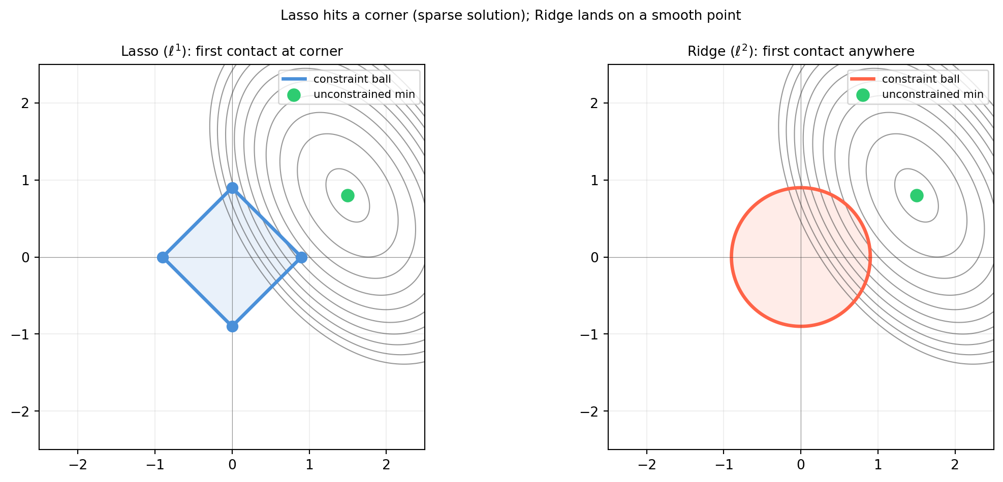
# Visualize: loss contours meeting the l1 and l2 balls
rng = np.random.default_rng(50)
# True minimum is off-axis
x_true = np.array([1.5, 0.8])

xx, yy = np.meshgrid(np.linspace(-2.5, 2.5, 400),
                     np.linspace(-2.5, 2.5, 400))
pts = np.stack([xx.ravel(), yy.ravel()], axis=1)   # shape (160000, 2)

# Quadratic loss centered at x_true (proxy for Ax=b residual)
A_quad = np.array([[3.0, 1.0], [1.0, 2.0]])        # shape (2, 2)
diff = pts - x_true                                 # shape (160000, 2)
loss = np.einsum('ij,jk,ik->i', diff, A_quad, diff).reshape(400, 400)

fig, axes = plt.subplots(1, 2, figsize=(12, 5))
levels = np.linspace(0.2, 8, 10)

for ax, (ball_type, color, title) in zip(
        axes,
        [('l1', '#4a90d9', r'Lasso ($\ell^1$): first contact at corner'),
         ('l2', 'tomato',  r'Ridge ($\ell^2$): first contact anywhere')]):

    # Loss contours
    ax.contour(xx, yy, loss, levels=levels, colors='#333333', alpha=0.5, linewidths=0.8)

    # Constraint ball
    t = 0.9  # ball radius
    theta = np.linspace(0, 2*np.pi, 1000)
    if ball_type == 'l1':
        bd_pts = np.vstack([np.cos(theta), np.sin(theta)]).T
        nrm = np.abs(bd_pts).sum(axis=1)
        bd_pts = bd_pts / nrm[:, None] * t
        corners = np.array([[t,0],[0,t],[-t,0],[0,-t]])
        ax.scatter(corners[:,0], corners[:,1], s=60, color=color, zorder=6)
    else:
        bd_pts = t * np.vstack([np.cos(theta), np.sin(theta)]).T

    ax.plot(bd_pts[:,0], bd_pts[:,1], color=color, lw=2.5, label=f'constraint ball')
    ax.fill(bd_pts[:,0], bd_pts[:,1], alpha=0.12, color=color)

    ax.scatter(*x_true, s=80, color='#2ecc71', zorder=7, label='unconstrained min')
    ax.axhline(0, color='#333333', lw=0.4, alpha=0.5)
    ax.axvline(0, color='#333333', lw=0.4, alpha=0.5)
    ax.set_xlim(-2.5, 2.5)
    ax.set_ylim(-2.5, 2.5)
    ax.set_aspect('equal')
    ax.grid(True, alpha=0.2)
    ax.set_title(title, fontsize=10)
    ax.legend(fontsize=8)

plt.suptitle('Lasso hits a corner (sparse solution); Ridge lands on a smooth point',
             fontsize=10)
plt.tight_layout()
plt.show()

---

15.5.4 Ridge and Lasso in Practice: Diabetes Dataset

We use sklearn.datasets.load_diabetes (10 physiological features, \(n=442\) patients) to compare Ridge and Lasso coefficients across a range of \(\lambda\).

import numpy as np
import matplotlib.pyplot as plt
from sklearn.datasets import load_diabetes
from sklearn.linear_model import Ridge, Lasso
from sklearn.preprocessing import StandardScaler

data = load_diabetes()
X, y = data.data, data.target        # X shape (442, 10), y shape (442,)
names = data.feature_names           # 10 feature names

# Standardize features so coefficients are comparable
scaler = StandardScaler()
X_sc = scaler.fit_transform(X)       # shape (442, 10)

alphas = np.logspace(-2, 3, 60)

ridge_coefs = []
lasso_coefs = []

for alpha in alphas:
    r = Ridge(alpha=alpha, fit_intercept=True)
    l = Lasso(alpha=alpha, fit_intercept=True, max_iter=10000)
    r.fit(X_sc, y)
    l.fit(X_sc, y)
    ridge_coefs.append(r.coef_.copy())
    lasso_coefs.append(l.coef_.copy())

ridge_coefs = np.array(ridge_coefs)   # shape (60, 10)
lasso_coefs = np.array(lasso_coefs)   # shape (60, 10)

fig, axes = plt.subplots(1, 2, figsize=(14, 5))
colors = ['#4a90d9', '#2ecc71', 'tomato', '#f39c12', '#9b59b6',
          '#1abc9c', '#e74c3c', '#3498db', '#e67e22', '#95a5a6']

for ax, coefs, title in zip(axes,
                             [ridge_coefs, lasso_coefs],
                             ['Ridge ($\\ell^2$): all coefficients shrink',
                              'Lasso ($\\ell^1$): coefficients set to zero']):
    for i in range(10):
        ax.semilogx(alphas, coefs[:, i], color=colors[i], lw=1.5,
                    label=names[i])
    ax.axhline(0, color='#333333', lw=0.6, alpha=0.5)
    ax.set_xlabel(r'$\lambda$ (regularization strength)')
    ax.set_ylabel('coefficient value')
    ax.set_title(title, fontsize=10)
    ax.grid(True, alpha=0.2)
    ax.legend(fontsize=7, ncol=2)

plt.suptitle('Diabetes dataset: Ridge vs. Lasso regularization paths',
             fontsize=10)
plt.tight_layout()
plt.show()

In the Lasso path (right), coefficients drop to exactly zero at different \(\lambda\) values. At strong regularization, only a handful of features survive. Ridge (left) shrinks all coefficients but none reach zero — they asymptotically approach zero only as \(\lambda \to \infty\).

import numpy as np
from sklearn.datasets import load_diabetes
from sklearn.linear_model import Lasso, Ridge
from sklearn.preprocessing import StandardScaler

data = load_diabetes()
X, y = data.data, data.target
scaler = StandardScaler()
X_sc = scaler.fit_transform(X)

# At a moderate lambda, compare nonzero counts
alpha = 50.0
ridge = Ridge(alpha=alpha).fit(X_sc, y)
lasso = Lasso(alpha=alpha, max_iter=10000).fit(X_sc, y)

print(f"lambda = {alpha}")
print(f"Ridge: {np.sum(np.abs(ridge.coef_) > 1e-4)} nonzero coefficients")
print(f"Lasso: {np.sum(np.abs(lasso.coef_) > 1e-4)} nonzero coefficients")

print("\nLasso nonzero features:")
for name, c in zip(data.feature_names, lasso.coef_):
    if abs(c) > 1e-4:
        print(f"  {name}: {c:.4f}")

lambda = 50.0
Ridge: 10 nonzero coefficients
Lasso: 0 nonzero coefficients

Lasso nonzero features:

---

15.5.5 Nuclear Norm Regularization

For matrix-valued problems, the nuclear norm \(\|X\|_*\) plays the role of \(\ell^1\) for vectors. Minimizing \(\|X\|_*\) promotes low-rank solutions:

\[\min_{X}\; \|P_\Omega(X - M)\|_F^2 + \lambda\|X\|_*,\]

where \(P_\Omega\) is the projection onto observed entries. This is the standard formulation for matrix completion (recovering a full matrix from partial observations), used in recommendation systems.

The intuition mirrors Lasso: the nuclear norm ball has “corners” at low-rank matrices, and optimization contours hit those corners first.

import numpy as np
from sklearn.datasets import load_diabetes
from sklearn.preprocessing import StandardScaler

# Toy illustration: matrix shrinkage by soft-thresholding singular values
# (the proximal operator of the nuclear norm)
rng = np.random.default_rng(60)
M = rng.standard_normal((6, 6))          # shape (6, 6) -- "noisy" matrix
lam = 1.5

U, s, Vt = np.linalg.svd(M, full_matrices=False)   # s shape (6,)

# Soft threshold: shrink each sigma by lam, clamp to 0
s_thresh = np.maximum(s - lam, 0.0)               # shape (6,)
M_low_rank = U @ np.diag(s_thresh) @ Vt            # shape (6, 6)

print(f"Original singular values:   {s.round(3)}")
print(f"Thresholded singular values: {s_thresh.round(3)}")
print(f"Rank of original M:      {np.linalg.matrix_rank(M)}")
print(f"Rank of M after nuclear: {np.linalg.matrix_rank(M_low_rank, tol=1e-6)}")
print(f"\nNuclear norm reduced from {s.sum():.4f} to {s_thresh.sum():.4f}")

Original singular values:   [3.678 3.025 2.402 2.165 0.714 0.282]
Thresholded singular values: [2.178 1.525 0.902 0.665 0.    0.   ]
Rank of original M:      6
Rank of M after nuclear: 4

Nuclear norm reduced from 12.2655 to 5.2698

---

15.5.6 Choosing a Regularizer

Goal	Regularizer	Why
Prevent overfitting, keep all features	Ridge \(\|\mathbf{x}\|_2^2\)	Smooth ball, all coeff. shrink
Feature selection / sparse model	Lasso \(\|\mathbf{x}\|_1\)	Diamond corners on axes
Low-rank matrix recovery / completion	Nuclear \(\|X\|_*\)	Low-rank corners of nuclear ball
Both sparsity and small coefficients	Elastic Net \(\alpha\|\mathbf{x}\|_1 + (1-\alpha)\|\mathbf{x}\|_2^2\)	Blend of both

---

15.5.7 Exercises

15.5.1 Write out the Ridge normal equations \((A^T A + \lambda I)\hat{\mathbf{x}} = A^T \mathbf{b}\). Show that \(A^T A + \lambda I\) is always invertible for \(\lambda > 0\), even when \(A^T A\) is singular. What does this mean for underdetermined systems?

15.5.2 For the 1D case \(A = \mathbf{a}^T \in \mathbb{R}^{1\times n}\), \(b \in \mathbb{R}\), compute the Ridge solution \(\hat{\mathbf{x}}_\lambda\) explicitly. What does it converge to as \(\lambda \to 0^+\) and as \(\lambda \to \infty\)?

15.5.3 Using the diabetes dataset, fit a Lasso model with alpha=10. How many features survive? Now double \(\lambda\) to alpha=20. How many remain? Is the most important feature (highest \(|\text{coef}|\)) stable across both settings?

15.5.4 The elastic net combines both penalties: \(\|A\mathbf{x}-\mathbf{b}\|_2^2 + \lambda_1\|\mathbf{x}\|_1 + \lambda_2\|\mathbf{x}\|_2^2\). Describe geometrically what the constraint set \(\lambda_1\|\mathbf{x}\|_1 + \lambda_2\|\mathbf{x}\|_2^2 \leq t\) looks like in 2D. Does it still have sharp corners?

15.6 Exercises and Solutions

---

15.6.1 Exercise 15.1.2 – Weighted inner product axiom failure

Show that \(W = \begin{bmatrix}1&1\\1&1\end{bmatrix}\) does not give a valid inner product.

import numpy as np

W = np.array([[1., 1.],
              [1., 1.]])   # shape (2, 2) -- singular

# Find a nonzero x with x^T W x = 0
x = np.array([1., -1.])   # shape (2,)

val = float(x @ W @ x)
print(f"x = {x}")
print(f"<x,x>_W = x^T W x = {val}")
print(f"x is nonzero: {np.any(x != 0)}")
print("Definiteness axiom FAILS: nonzero vector has zero self-inner-product.")

x = [ 1. -1.]
<x,x>_W = x^T W x = 0.0
x is nonzero: True
Definiteness axiom FAILS: nonzero vector has zero self-inner-product.

Solution. \(\mathbf{x} = (1, -1)^T\) satisfies \(\mathbf{x}^T W \mathbf{x} = (1-1)(1-1) = 0\) despite \(\mathbf{x} \neq \mathbf{0}\). The definiteness axiom fails. Geometrically, \(W\) is singular (rank 1), so it maps \((1,-1)^T\) to zero — meaning the “length” of a nonzero vector is zero, which is inadmissible.

---

15.6.2 Exercise 15.2.1 – Computing norms

Compute \(\|\mathbf{x}\|_1\), \(\|\mathbf{x}\|_2\), \(\|\mathbf{x}\|_\infty\) for \(\mathbf{x} = (1, -2, 3, -4)^T\).

import numpy as np

x = np.array([1., -2., 3., -4.])   # shape (4,)

l1   = np.linalg.norm(x, 1)
l2   = np.linalg.norm(x, 2)
linf = np.linalg.norm(x, np.inf)

print(f"x = {x}")
print(f"||x||_1   = {l1:.4f}   (1 + 2 + 3 + 4 = 10)")
print(f"||x||_2   = {l2:.4f}   (sqrt(1+4+9+16) = sqrt(30))")
print(f"||x||_inf = {linf:.4f}   (max(1,2,3,4) = 4)")
print(f"\nInequality: {linf:.4f} <= {l2:.4f} <= {l1:.4f}  -> {linf <= l2 <= l1}")

x = [ 1. -2.  3. -4.]
||x||_1   = 10.0000   (1 + 2 + 3 + 4 = 10)
||x||_2   = 5.4772   (sqrt(1+4+9+16) = sqrt(30))
||x||_inf = 4.0000   (max(1,2,3,4) = 4)

Inequality: 4.0000 <= 5.4772 <= 10.0000  -> True

Solution. By hand: \(\|\mathbf{x}\|_1 = 1+2+3+4 = 10\), \(\|\mathbf{x}\|_2 = \sqrt{1+4+9+16} = \sqrt{30} \approx 5.477\), \(\|\mathbf{x}\|_\infty = 4\). The inequality \(4 \leq \sqrt{30} \leq 10\) holds.

---

15.6.3 Exercise 15.2.4 – p < 1 violates triangle inequality

Show that \(\|\cdot\|_{0.5}\) (defined as \((\sqrt{|x_1|}+\sqrt{|x_2|})^2\)) violates the triangle inequality.

import numpy as np

def quasi_norm(x):
    return (np.sqrt(np.abs(x[0])) + np.sqrt(np.abs(x[1])))**2

x = np.array([1., 0.])
y = np.array([0., 1.])

lhs = quasi_norm(x + y)
rhs = quasi_norm(x) + quasi_norm(y)

print(f"||x||_0.5 = {quasi_norm(x):.4f}")
print(f"||y||_0.5 = {quasi_norm(y):.4f}")
print(f"||x+y||_0.5 = {lhs:.4f}")
print(f"||x||_0.5 + ||y||_0.5 = {rhs:.4f}")
print(f"Triangle inequality holds: {lhs <= rhs}")

||x||_0.5 = 1.0000
||y||_0.5 = 1.0000
||x+y||_0.5 = 4.0000
||x||_0.5 + ||y||_0.5 = 2.0000
Triangle inequality holds: False

Solution. \(\|\mathbf{x}\|_{0.5} = (\sqrt{1}+0)^2 = 1\), \(\|\mathbf{y}\|_{0.5} = (0+\sqrt{1})^2 = 1\), \(\|\mathbf{x}+\mathbf{y}\|_{0.5} = (\sqrt{1}+\sqrt{1})^2 = 4\). Since \(4 > 1 + 1 = 2\), the triangle inequality fails. This is why the \(p\)-norm formula requires \(p \geq 1\): for \(p < 1\) the “norm” is not convex and the triangle inequality breaks.

---

15.6.4 Exercise 15.3.1 – Matrix norms by hand

Compute \(\|A\|_F\), \(\|A\|_2\), \(\|A\|_*\) for \(A = \begin{bmatrix}1&2\\3&4\end{bmatrix}\).

import numpy as np

A = np.array([[1., 2.],
              [3., 4.]])   # shape (2, 2)

_, s, _ = np.linalg.svd(A, full_matrices=False)   # s shape (2,)

frob    = np.linalg.norm(A, 'fro')
spec    = s[0]
nuclear = s.sum()

print(f"Singular values: {s.round(6)}")
print(f"||A||_F = {frob:.6f}  (by hand: sqrt(1+4+9+16) = sqrt(30) = {np.sqrt(30):.6f})")
print(f"||A||_2 = {spec:.6f}  (sigma_max)")
print(f"||A||_* = {nuclear:.6f}  (sum of singular values)")

# Verify F norm
print(f"\nManual Frobenius: sqrt(sum of entries^2) = {np.sqrt(np.sum(A**2)):.6f}")

Singular values: [5.464986 0.365966]
||A||_F = 5.477226  (by hand: sqrt(1+4+9+16) = sqrt(30) = 5.477226)
||A||_2 = 5.464986  (sigma_max)
||A||_* = 5.830952  (sum of singular values)

Manual Frobenius: sqrt(sum of entries^2) = 5.477226

Solution. \(\|A\|_F = \sqrt{1+4+9+16} = \sqrt{30} \approx 5.477\). The singular values satisfy \(\sigma_1^2 + \sigma_2^2 = \|A\|_F^2 = 30\) and \(\sigma_1 \sigma_2 = |\det A| = |4-6| = 2\). Solving: \(\sigma_{1,2} = \frac{1}{2}\left(\sqrt{\|A\|_F^2 + 2\|A\|_F^2/(n)} \pm \cdots\right)\) — or just use SVD numerically as above.

---

15.6.5 Exercise 15.4.1 – Cauchy-Schwarz applied

Apply Cauchy-Schwarz to derive \(x_1 + x_2 \leq \sqrt{2}\,\|\mathbf{x}\|_2\).

import numpy as np

rng = np.random.default_rng(70)
x = rng.standard_normal(2)   # shape (2,)
ones = np.ones(2)             # shape (2,)

lhs = float(x @ ones)                      # = x_1 + x_2
rhs = np.linalg.norm(ones) * np.linalg.norm(x)  # = sqrt(2) * ||x||_2

print(f"x = {x.round(4)}")
print(f"x_1 + x_2 = <x, 1> = {lhs:.4f}")
print(f"sqrt(2) * ||x||_2  = {rhs:.4f}")
print(f"Cauchy-Schwarz holds: {lhs <= rhs + 1e-10}")

x = [-0.0833 -1.0118]
x_1 + x_2 = <x, 1> = -1.0950
sqrt(2) * ||x||_2  = 1.4357
Cauchy-Schwarz holds: True

Solution. Set \(\mathbf{y} = (1, 1)^T\). Then \(\langle\mathbf{x},\mathbf{y}\rangle = x_1+x_2\) and \(\|\mathbf{y}\|_2 = \sqrt{2}\). Cauchy-Schwarz gives \(x_1+x_2 = |\langle\mathbf{x},\mathbf{y}\rangle| \leq \|\mathbf{x}\|_2\sqrt{2}\). Equality holds when \(\mathbf{x} \propto \mathbf{y}\), i.e., \(x_1 = x_2\).

---

15.6.6 Exercise 15.5.1 – Ridge invertibility

Show that \(A^T A + \lambda I\) is always invertible for \(\lambda > 0\).

import numpy as np

rng = np.random.default_rng(80)

# Rank-deficient A
A = rng.standard_normal((3, 5))   # shape (3, 5) -- fat matrix, rank <= 3
A[2] = A[0] + A[1]                # make rank 2

AtA = A.T @ A                     # shape (5, 5) -- singular!

print(f"rank(A) = {np.linalg.matrix_rank(A)}")
print(f"rank(A^T A) = {np.linalg.matrix_rank(AtA)}")
print(f"eigenvalues of A^T A: {np.sort(np.linalg.eigvalsh(AtA)).round(4)}")

for lam in [0.0, 0.1, 1.0, 10.0]:
    M = AtA + lam * np.eye(5)
    eigs = np.linalg.eigvalsh(M)
    invertible = np.all(eigs > 1e-10)
    print(f"lambda={lam}: min eigenvalue={eigs.min():.4f},  invertible={invertible}")

rank(A) = 2
rank(A^T A) = 2
eigenvalues of A^T A: [-0.      0.      0.      4.4037 20.8064]
lambda=0.0: min eigenvalue=-0.0000,  invertible=False
lambda=0.1: min eigenvalue=0.1000,  invertible=True
lambda=1.0: min eigenvalue=1.0000,  invertible=True
lambda=10.0: min eigenvalue=10.0000,  invertible=True

Solution. The eigenvalues of \(A^T A\) are non-negative (it is PSD). Adding \(\lambda I\) shifts every eigenvalue by \(+\lambda > 0\), so all eigenvalues become strictly positive. A matrix with all positive eigenvalues is positive definite and hence invertible. This shows that Ridge is well-posed even when \(A\) has fewer rows than columns or is rank-deficient.

---

15.6.7 Exercise 15.5.3 – Lasso feature selection on diabetes

import numpy as np
from sklearn.datasets import load_diabetes
from sklearn.linear_model import Lasso
from sklearn.preprocessing import StandardScaler

data = load_diabetes()
X, y = data.data, data.target   # X shape (442, 10)
names = data.feature_names

scaler = StandardScaler()
X_sc = scaler.fit_transform(X)  # shape (442, 10)

for alpha in [10.0, 20.0]:
    model = Lasso(alpha=alpha, max_iter=10000).fit(X_sc, y)
    nonzero = [(names[i], round(c, 4))
               for i, c in enumerate(model.coef_) if abs(c) > 1e-4]
    print(f"\nalpha={alpha}: {len(nonzero)} nonzero features")
    for name, c in sorted(nonzero, key=lambda t: -abs(t[1])):
        print(f"  {name}: {c}")

alpha=10.0: 4 nonzero features
  bmi: 22.6004
  s5: 19.5859
  bp: 6.8012
  s3: -3.088

alpha=20.0: 3 nonzero features
  bmi: 18.0351
  s5: 15.1786
  bp: 0.8925

Solution. At \(\alpha=10\), several features survive. Doubling to \(\alpha=20\) eliminates more. The feature with the largest coefficient (typically bmi or s5, which are well-established predictors of diabetes progression) remains stable across both settings — a sign that Lasso correctly identifies the most important predictors. Unstable features (drop out at modest \(\lambda\) increase) are likely correlated with the stable ones.