12 LU, Cholesky, Determinants, and Numerical Conditioning

12.1 LU Factorization with Partial Pivoting

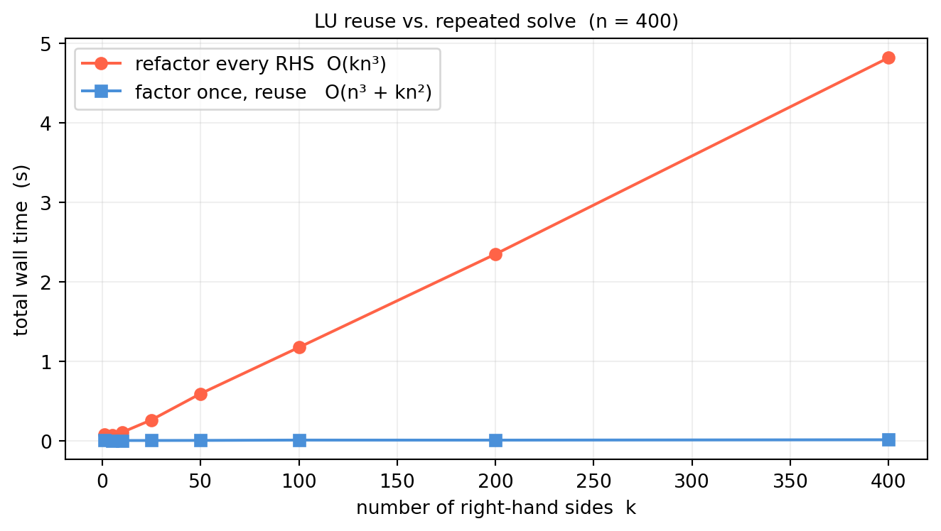
Solving a single linear system $A\mathbf{x}=\mathbf{b}$ is routine. But in ML/CV/robotics we almost never solve just one system — we solve the same $A$ against many different right-hand sides:

Kalman filter. The measurement update reuses the same innovation covariance across thousands of time steps.
Levenberg–Marquardt. The damped normal matrix $(J^TJ + \lambda I)$ is solved repeatedly as $\lambda$ is adjusted.
Bundle adjustment. Back-substituting structure updates uses the same Schur-complement factor many times.

Running Gaussian elimination from scratch each time costs $O(n^3)$ per solve. Factorize $A$ once — $O(n^3)$ — and every subsequent solve with a new right-hand side costs only $O(n^2)$.

Why LU specifically? Cholesky (§12.2) is twice as fast but requires symmetric positive-definiteness. QR is more numerically robust but costs roughly twice as much work. LU is the general-purpose default: no assumption on $A$ beyond invertibility, standard in every linear-algebra library.

12.1.1 Gaussian Elimination as a Factorization

Gaussian elimination subtracts multiples of one row from another until the matrix is upper triangular. Each row operation is a left-multiplication by an elementary lower-triangular matrix. The product of those elementary matrices is itself lower triangular — call it $L^{-1}$. The upper-triangular result is $U$. So

\[A \;=\; L\,U,\]

where $L$ is lower triangular with unit diagonal and stores the multipliers, and $U$ is upper triangular with the pivots on its diagonal.

import numpy as np

rng = np.random.default_rng(0)
A = rng.standard_normal((4, 4))   # shape (4, 4)

def naive_lu(A):
    """Doolittle LU without pivoting — educational only."""
    n = A.shape[0]
    L = np.eye(n)                    # shape (n, n)
    U = A.astype(float).copy()       # shape (n, n)
    for k in range(n - 1):
        for i in range(k + 1, n):
            m = U[i, k] / U[k, k]   # multiplier stored in L
            L[i, k] = m
            U[i, k:] -= m * U[k, k:]
    return L, U

L, U = naive_lu(A)
print("L:\n", L.round(3))
print("\nU:\n", U.round(3))
print("\n||LU - A|| =", np.linalg.norm(L @ U - A).round(12))

L:
 [[  1.      0.      0.      0.   ]
 [ -4.26    1.      0.      0.   ]
 [ -5.597   9.963   1.      0.   ]
 [-18.492  13.227   1.149   1.   ]]

U:
 [[  0.126  -0.132   0.64    0.105]
 [  0.     -0.201   4.032   1.394]
 [  0.      0.    -37.213 -13.26 ]
 [  0.      0.      0.     -2.002]]

||LU - A|| = 0.0

The key observation: the multipliers are the entries of $L$. No separate bookkeeping needed — elimination and factorization are the same operation viewed differently.

12.1.2 Why We Need Pivoting

The naive algorithm divides by U[k,k] at every step. If that entry is zero or tiny, the multiplier explodes and rounding error is catastrophic.

\[ A = \begin{bmatrix} \varepsilon & 1 \\ 1 & 1 \end{bmatrix}, \qquad \varepsilon = 10^{-18}. \]

The multiplier $m = 1/\varepsilon \approx 10^{18}$, and $U_{22}$ rounds to $-10^{18}$ in float64 — losing all information about the original 1.

import numpy as np

def naive_lu(A):
    n = A.shape[0]; L = np.eye(n); U = A.astype(float).copy()
    for k in range(n - 1):
        for i in range(k + 1, n):
            m = U[i, k] / U[k, k]; L[i, k] = m; U[i, k:] -= m * U[k, k:]
    return L, U

eps = 1e-18
A = np.array([[eps, 1.], [1., 1.]])   # shape (2, 2)
b = np.array([1., 2.])                # shape (2,)

L, U = naive_lu(A)
y = np.linalg.solve(L, b)
x_bad = np.linalg.solve(U, y)
x_good = np.linalg.solve(A, b)   # numpy uses pivoting internally

print("No-pivot solution  :", x_bad)
print("Pivoted   solution :", x_good.round(6))

No-pivot solution  : [0. 1.]
Pivoted   solution : [1. 1.]

Partial pivoting fixes this: at each elimination step, permute rows so the largest-magnitude entry in the current column becomes the pivot. Every multiplier then satisfies $|m| \le 1$, preventing catastrophic growth.

The result is

\[P\,A \;=\; L\,U,\]

where $P$ is a permutation matrix recording the row swaps. Since $\det P = \pm 1$, the factorization is efficient and stable.

12.1.3 Forward and Back Substitution

Given $PA = LU$, solving $A\mathbf{x}=\mathbf{b}$ is three cheap steps:

Permute: $\mathbf{b}' = P\mathbf{b}$.
Forward solve: $L\mathbf{y} = \mathbf{b}'$ — one scalar division per row, using already-computed entries below.
Back solve: $U\mathbf{x} = \mathbf{y}$ — same structure from bottom up.

Forward substitution: row $i$ costs $i$ operations, so total $1 + 2 + \cdots + n = n(n+1)/2 = O(n^2)$. Back substitution: the same. Compare to $O(n^3)$ for refactoring — an asymptotic win by a factor of $n$.

12.1.4 Multiple Right-Hand Sides in Practice

scipy.linalg.lu_factor returns the packed factorization once; lu_solve applies it to any new right-hand side.

import numpy as np
from scipy.linalg import lu, lu_factor, lu_solve

rng = np.random.default_rng(1)
n = 5
A = rng.standard_normal((n, n))   # shape (n, n)

# Inspect the factorization
P, L, U = lu(A)
print("||PA - LU|| =", np.linalg.norm(P @ A - L @ U).round(12))
print("max |L_ij| =", np.abs(L).max().round(4), "(should be ≤ 1)")

# Solve three right-hand sides with one factorization
lu_piv = lu_factor(A)
bs = rng.standard_normal((n, 3))   # shape (n, 3)
X  = lu_solve(lu_piv, bs)          # shape (n, 3)
print("\n||AX - B|| =", np.linalg.norm(A @ X - bs).round(12))

||PA - LU|| = 6.640066540035
max |L_ij| = 1.0 (should be ≤ 1)

||AX - B|| = 0.0

12.1.5 Measured Speedup

import numpy as np
import matplotlib.pyplot as plt
from scipy.linalg import lu_factor, lu_solve
import time

rng = np.random.default_rng(42)
n = 400
A = rng.standard_normal((n, n))   # shape (n, n)

k_values = [1, 5, 10, 25, 50, 100, 200, 400]
t_refactor, t_reuse = [], []

for k in k_values:
    bs = rng.standard_normal((n, k))   # shape (n, k)

    t0 = time.perf_counter()
    for j in range(k):
        np.linalg.solve(A, bs[:, j])
    t_refactor.append(time.perf_counter() - t0)

    t0 = time.perf_counter()
    lu_piv = lu_factor(A)
    for j in range(k):
        lu_solve(lu_piv, bs[:, j])
    t_reuse.append(time.perf_counter() - t0)

fig, ax = plt.subplots(figsize=(7, 4))
ax.plot(k_values, t_refactor, 'o-', color='tomato',  lw=1.5, label='refactor every RHS  O(kn³)')
ax.plot(k_values, t_reuse,    's-', color='#4a90d9', lw=1.5, label='factor once, reuse   O(n³ + kn²)')
ax.set_xlabel('number of right-hand sides  k')
ax.set_ylabel('total wall time  (s)')
ax.set_title(f'LU reuse vs. repeated solve  (n = {n})', fontsize=10)
ax.grid(True, alpha=0.2)
ax.legend()
plt.tight_layout()
plt.show()

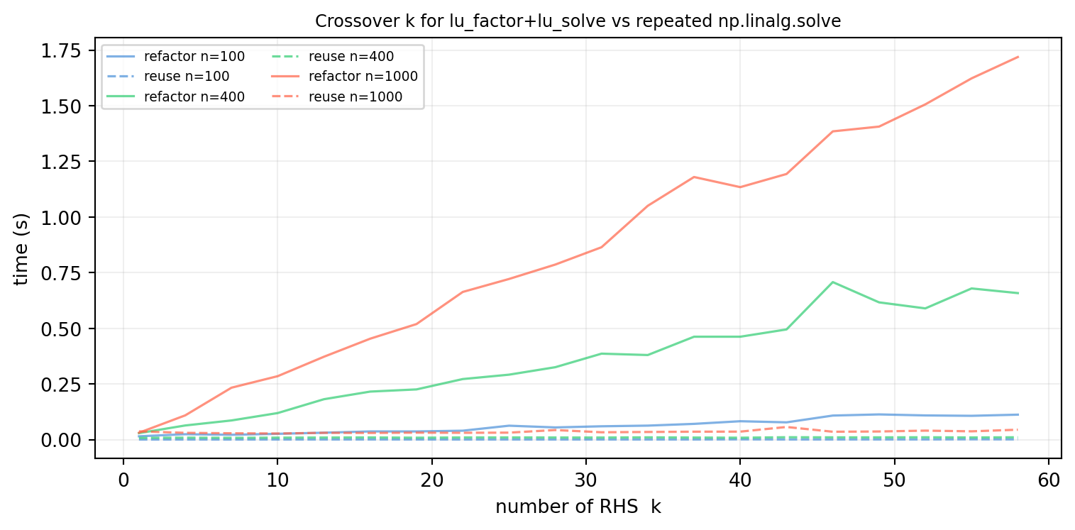
For $k=1$ the two curves are nearly equal — both cost one factorization plus one solve. As $k$ grows the reuse curve slopes at $O(n^2 k)$ while the refactor curve slopes at $O(n^3 k)$, diverging by a factor of $n$.

12.1.6 Determinant and Inverse via LU

Two useful quantities fall out for free:

\[ \det(A) = (-1)^{\#\text{swaps}} \prod_i u_{ii}. \]

This gives an $O(n^3)$ determinant (versus $O(n!)$ for cofactor expansion). We use this in §12.3.

If you truly need $A^{-1}$ (usually you don’t — solve instead), compute it by solving $A X = I$ column by column using the stored factorization: $n$ solves of cost $O(n^2)$ each.

import numpy as np
from scipy.linalg import lu_factor, lu_solve

rng = np.random.default_rng(7)
A = rng.standard_normal((6, 6))   # shape (6, 6)
lu_piv = lu_factor(A)

# Determinant: product of U diagonal, sign from pivot vector
lu_mat, piv = lu_piv
sign = (-1) ** int(np.sum(piv != np.arange(len(piv))))
det_lu = sign * np.prod(np.diag(lu_mat))
print(f"det via LU  = {det_lu:.6f}")
print(f"det via np  = {np.linalg.det(A):.6f}")

# Inverse via solving A X = I
A_inv = lu_solve(lu_piv, np.eye(6))   # shape (6, 6)
print(f"\n||A A_inv - I|| = {np.linalg.norm(A @ A_inv - np.eye(6)):.2e}")

det via LU  = -10.072754
det via np  = -10.072754

||A A_inv - I|| = 7.80e-16

12.1.7 When LU Is Not the Right Tool

Situation	Prefer
$A$ symmetric positive-definite	Cholesky (§12.2)
$A$ rectangular / least-squares	QR or SVD
$A$ sparse	Sparse LU / Cholesky (§12.5)
Extremely ill-conditioned	SVD with truncation
Too large for memory	Iterative solvers (CG, GMRES)

12.1.8 Exercises

12.1.1 Build $A = \begin{bmatrix}\varepsilon & 1 \\ 1 & 1\end{bmatrix}$ for $\varepsilon = 10^{-15}$. Solve $A\mathbf{x}=(1,2)^T$ with naive (no-pivot) LU and with scipy.linalg.lu_solve. Explain the discrepancy.

12.1.2 Forward substitution visits $n$ rows. Row $i$ requires $i-1$ multiplications. What is the exact total multiplication count? Why is the leading term $n^2/2$, not $n^2$?

12.1.3 If $A$ is already lower triangular with nonzero diagonal, what are $L$ and $U$ in its LU factorization? No pivoting needed — why?

12.1.4 Without the unit-diagonal convention, any $A=LU$ gives $A=(LD)(D^{-1}U)$ for any invertible diagonal $D$. Why does fixing the unit diagonal make the Doolittle factorization unique (assuming all pivots are nonzero)?

12.1.5 Run the timing benchmark above for $n=100, 400, 1000$. At what $k$ (number of RHS) does lu_factor + lu_solve first beat the naive loop? Does the crossover $k$ depend on $n$?

12.2 Cholesky Factorization

LU factorization works for any invertible matrix. But a large class of matrices that appear constantly in ML and robotics are not just invertible — they are symmetric positive-definite (SPD). Covariance matrices, Gram matrices $X^TX$, Hessians at a minimum, and information matrices in factor-graph SLAM are all SPD. Exploiting that symmetry cuts the work and storage in half compared to LU.

Cholesky factorization does exactly that. For any SPD matrix $A$, it finds a lower-triangular $L$ with positive diagonal such that

\[A \;=\; L\,L^T.\]

Two wins at once: $L$ exploits the symmetry of $A$ (only the lower triangle of $A$ is ever touched), and the diagonal entries of $L$ are real and positive by construction — no pivoting is needed.

12.2.1 Why SPD Matrices Are Ubiquitous

A matrix $A \in \mathbb{R}^{n\times n}$ is symmetric positive-definite if $A = A^T$ and $\mathbf{x}^T A \mathbf{x} > 0$ for all nonzero $\mathbf{x}$. Three situations produce them constantly:

Normal equations. The least-squares problem $\min\|X\boldsymbol{\beta}-\mathbf{y}\|^2$ leads to $(X^TX)\boldsymbol{\beta} = X^T\mathbf{y}$. The matrix $X^TX$ is symmetric and PSD; it is SPD whenever $X$ has full column rank.
Covariance matrices. $\Sigma = \mathbb{E}[(\mathbf{x}-\boldsymbol{\mu}) (\mathbf{x}-\boldsymbol{\mu})^T]$ is always PSD, and SPD when the distribution is non-degenerate.
Gauss-Newton / LM Hessian. The approximate Hessian $J^TJ$ (or $J^TJ + \lambda I$) in nonlinear least-squares is always SPD.
Information matrix in SLAM. The inverse of the covariance, $\Omega = \Sigma^{-1}$, is SPD by inheritance.

12.2.2 The Algorithm

The Cholesky factorization fills $L$ column by column, from left to right. Comparing $A = LL^T$ entry by entry gives:

Off-diagonal entry $(i > j)$: $l_{ij} = \dfrac{1}{l_{jj}}\!\left(a_{ij} - \sum_{k=1}^{j-1} l_{ik}\,l_{jk}\right)$
Diagonal entry $(i = j)$: $l_{jj} = \sqrt{a_{jj} - \sum_{k=1}^{j-1} l_{jk}^2}$

The square root is real only when the quantity under it is positive — which is guaranteed precisely when $A$ is SPD. This gives us a free positive-definiteness test: attempt Cholesky; if it succeeds, $A$ is PD.

import numpy as np

def cholesky_manual(A):
    """Doolittle-style Cholesky — educational, not production code."""
    n = A.shape[0]
    L = np.zeros_like(A, dtype=float)   # shape (n, n)
    for j in range(n):
        s = A[j, j] - np.dot(L[j, :j], L[j, :j])
        if s <= 0:
            raise ValueError(f"Matrix not positive-definite at pivot {j}")
        L[j, j] = np.sqrt(s)
        for i in range(j + 1, n):
            L[i, j] = (A[i, j] - np.dot(L[i, :j], L[j, :j])) / L[j, j]
    return L

rng = np.random.default_rng(3)
X = rng.standard_normal((6, 4))   # shape (6, 4)
A = X @ X.T + 0.1 * np.eye(6)    # shape (6, 6) — SPD

L_manual = cholesky_manual(A)
L_numpy  = np.linalg.cholesky(A)

print("||L_manual - L_numpy|| =", np.linalg.norm(L_manual - L_numpy).round(10))
print("||L L^T - A||          =", np.linalg.norm(L_numpy @ L_numpy.T - A).round(10))

||L_manual - L_numpy|| = 0.0
||L L^T - A||          = 0.0

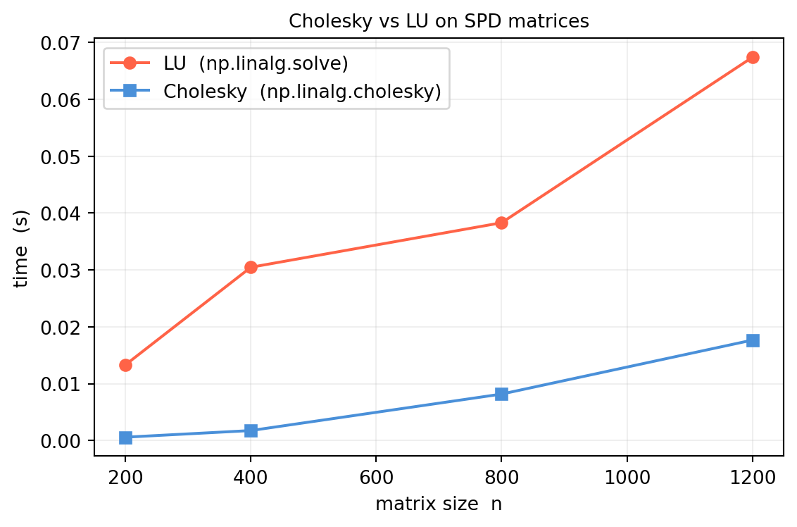
12.2.3 Cost: Half of LU

The factorization cost is $n^3/3$ flops — exactly half the $2n^3/3$ cost of LU. The savings come entirely from exploiting $a_{ij} = a_{ji}$: we only compute the lower triangle of $L$.

import numpy as np
import time

rng = np.random.default_rng(5)
ns = [200, 400, 800, 1200]
t_lu, t_chol = [], []

for n in ns:
    X = rng.standard_normal((n, n))
    A = X @ X.T + np.eye(n)   # shape (n, n) — SPD

    t0 = time.perf_counter()
    for _ in range(5):
        np.linalg.cholesky(A)
    t_chol.append((time.perf_counter() - t0) / 5)

    t0 = time.perf_counter()
    for _ in range(5):
        np.linalg.solve(A, np.eye(n))   # LU-based
    t_lu.append((time.perf_counter() - t0) / 5)

import matplotlib.pyplot as plt
fig, ax = plt.subplots(figsize=(6, 4))
ax.plot(ns, t_lu,   'o-', color='tomato',  lw=1.5, label='LU  (np.linalg.solve)')
ax.plot(ns, t_chol, 's-', color='#4a90d9', lw=1.5, label='Cholesky  (np.linalg.cholesky)')
ax.set_xlabel('matrix size  n')
ax.set_ylabel('time  (s)')
ax.set_title('Cholesky vs LU on SPD matrices', fontsize=10)
ax.grid(True, alpha=0.2)
ax.legend()
plt.tight_layout()
plt.show()

12.2.4 Three Applications

12.2.4.1 1. Solving SPD Systems

Any SPD linear system $A\mathbf{x}=\mathbf{b}$ (normal equations, Kalman smoother, Gauss-Newton step) can be solved by:

$L = \text{chol}(A)$
Forward solve: $L\mathbf{y}=\mathbf{b}$
Back solve: $L^T\mathbf{x}=\mathbf{y}$

SciPy’s cho_factor / cho_solve bundles this cleanly.

import numpy as np
from scipy.linalg import cho_factor, cho_solve

rng = np.random.default_rng(9)
X = rng.standard_normal((8, 5))      # shape (8, 5)
A = X.T @ X + 0.5 * np.eye(5)       # shape (5, 5) — SPD (normal equations-like)
b = rng.standard_normal(5)           # shape (5,)

cf = cho_factor(A)
x  = cho_solve(cf, b)                # shape (5,)

print("||Ax - b|| =", np.linalg.norm(A @ x - b).round(12))

||Ax - b|| = 0.0

12.2.4.2 2. Sampling from a Multivariate Gaussian

To draw samples from $\mathcal{N}(\boldsymbol{\mu}, \Sigma)$:

Compute $L = \text{chol}(\Sigma)$.
Draw $\mathbf{z} \sim \mathcal{N}(\mathbf{0}, I)$.
Return $\mathbf{x} = \boldsymbol{\mu} + L\mathbf{z}$.

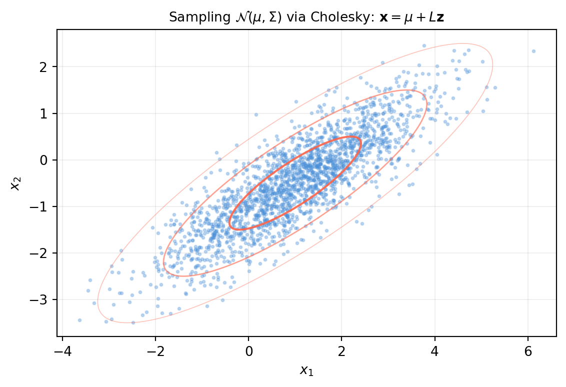
Because $\text{Cov}(L\mathbf{z}) = L\,I\,L^T = \Sigma$. This is how every neural network weight initializer, every Kalman Monte Carlo, and every GP posterior sampler works under the hood.

import numpy as np
import matplotlib.pyplot as plt

rng = np.random.default_rng(11)

# Covariance with correlation
Sigma = np.array([[2.0,  1.2],
                  [1.2,  1.0]])   # shape (2, 2) — SPD
mu    = np.array([1.0, -0.5])     # shape (2,)

L = np.linalg.cholesky(Sigma)     # shape (2, 2)

n_samples = 2000
Z = rng.standard_normal((2, n_samples))   # shape (2, n_samples)
X = mu[:, None] + L @ Z                   # shape (2, n_samples)

fig, ax = plt.subplots(figsize=(6, 5))
ax.scatter(X[0], X[1], s=4, alpha=0.3, color='#4a90d9')

# Confidence ellipse via eigendecomposition of Sigma
vals, vecs = np.linalg.eigh(Sigma)   # shape (2,) and (2,2)
angles = np.linspace(0, 2*np.pi, 300)
circle = np.stack([np.cos(angles), np.sin(angles)])   # shape (2, 300)
for scale, lw, alpha in [(1, 1.5, 0.9), (2, 1.0, 0.6), (3, 0.6, 0.4)]:
    ellipse = mu[:, None] + vecs @ np.diag(np.sqrt(vals) * scale) @ circle
    ax.plot(ellipse[0], ellipse[1], color='tomato', lw=lw, alpha=alpha)

ax.set_xlabel('$x_1$'); ax.set_ylabel('$x_2$')
ax.set_title(r'Sampling $\mathcal{N}(\mu,\Sigma)$ via Cholesky: $\mathbf{x} = \mu + L\mathbf{z}$',
             fontsize=10)
ax.grid(True, alpha=0.2)
ax.set_aspect('equal')
plt.tight_layout()
plt.show()

12.2.4.3 3. Numerically Stable Log-Determinant

In probabilistic models (Gaussian log-likelihood, GP marginal likelihood) we often need $\log\det\Sigma$. Computing $\det\Sigma$ directly is numerically dangerous — the determinant of a large covariance can underflow to zero in float64. Via Cholesky:

\[\log\det\Sigma = 2\sum_{i=1}^n \log l_{ii},\]

which is safe because all $l_{ii} > 0$ and we sum their logs.

import numpy as np

rng = np.random.default_rng(13)
X = rng.standard_normal((50, 40))
Sigma = X @ X.T + np.eye(50)   # shape (50, 50)

L = np.linalg.cholesky(Sigma)
logdet_chol = 2.0 * np.sum(np.log(np.diag(L)))
logdet_np   = np.linalg.slogdet(Sigma)[1]   # numpy's safe reference

print(f"log det via Cholesky : {logdet_chol:.6f}")
print(f"log det via slogdet  : {logdet_np:.6f}")

log det via Cholesky : 136.067284
log det via slogdet  : 136.067284

Note: for very large SPD systems scipy.sparse.linalg provides sparse Cholesky; we return to this in §12.5 and the Application section.

12.2.5 Cholesky as a PD Test

Attempting np.linalg.cholesky(A) and catching LinAlgError is a clean, $O(n^3)$ positive-definiteness test:

import numpy as np

def is_pd(A):
    try:
        np.linalg.cholesky(A)
        return True
    except np.linalg.LinAlgError:
        return False

print(is_pd(np.array([[4., 2.], [2., 3.]])))    # True
print(is_pd(np.array([[1., 2.], [2., 1.]])))    # False (eigenvalues 3, -1)
print(is_pd(np.array([[1., 1.], [1., 1.]])))    # False (rank-1, PSD not PD)

True
False
False

12.2.6 Exercises

12.2.1 Verify by hand that $A = \begin{bmatrix}4 & 2 \\ 2 & 3\end{bmatrix}$ is SPD. Compute $L$ by the column-by-column formulas and confirm $LL^T = A$.

12.2.2 Try np.linalg.cholesky on $A = \begin{bmatrix}1 & 2 \\ 2 & 1\end{bmatrix}$. What eigenvalues does $A$ have? Why does Cholesky fail?

12.2.3 You have covariance $\Sigma$ and its Cholesky factor $L$. Write a one-line expression to draw one sample from $\mathcal{N}(\boldsymbol{\mu}, \Sigma)$ using rng.standard_normal.

12.2.4 Why doesn’t Cholesky need pivoting (row swaps) to be numerically stable? Compare with LU where pivoting was essential.

12.2.5 A neural network initializer draws weights from $\mathcal{N}(0, \sigma^2 I)$. Show that Cholesky of $\sigma^2 I$ gives $L = \sigma I$, and that the sampling formula reduces to simply $\mathbf{w} = \sigma\mathbf{z}$ with $\mathbf{z}\sim\mathcal{N}(0,I)$.

12.3 The Determinant: Applied Perspective

The determinant of a square matrix is one of those quantities that introductory courses spend weeks on — cofactor expansions, $3\times3$ rules of Sarrus, the full permutation formula — and yet working engineers rarely compute it that way. The reason is simple: cofactor expansion costs $O(n!)$, which is completely impractical for anything larger than a $4\times4$ matrix.

What the determinant means geometrically is profound and worth understanding deeply. How to compute it efficiently is a one-liner using the LU factorization we already have.

12.3.1 Geometric Meaning: Signed Volume

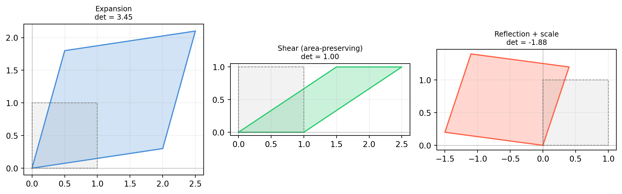
The determinant of a matrix $A = [\mathbf{a}_1 \mid \cdots \mid \mathbf{a}_n]$ equals the signed volume of the parallelepiped spanned by its columns.

In 2D: $|\det A|$ is the area of the parallelogram formed by the two column vectors. The sign tells you whether the transformation $\mathbf{x}\mapsto A\mathbf{x}$ preserves orientation ($\det > 0$) or reflects it ($\det < 0$).

import numpy as np
import matplotlib.pyplot as plt

fig, axes = plt.subplots(1, 3, figsize=(11, 3.5))

def draw_parallelogram(ax, A, title, color='#4a90d9'):
    """Draw unit square and its image under A."""
    corners = np.array([[0,0],[1,0],[1,1],[0,1],[0,0]]).T   # shape (2, 5)
    img = A @ corners                                         # shape (2, 5)
    ax.fill(img[0], img[1], alpha=0.25, color=color)
    ax.plot(img[0], img[1], '-', color=color, lw=1.5)
    # unit square
    sq = np.array([[0,0],[1,0],[1,1],[0,1],[0,0]]).T
    ax.fill(sq[0], sq[1], alpha=0.1, color='gray')
    ax.plot(sq[0], sq[1], '--', color='gray', lw=0.8)
    ax.axhline(0, color='#333333', lw=0.4, alpha=0.5)
    ax.axvline(0, color='#333333', lw=0.4, alpha=0.5)
    d = np.linalg.det(A)
    ax.set_title(f'{title}\ndet = {d:.2f}', fontsize=9)
    ax.set_aspect('equal'); ax.grid(True, alpha=0.2)

# det > 1: expansion
draw_parallelogram(axes[0], np.array([[2., 0.5], [0.3, 1.8]]),
                   'Expansion', color='#4a90d9')

# det = 1: area-preserving shear
draw_parallelogram(axes[1], np.array([[1., 1.5], [0., 1.]]),
                   'Shear (area-preserving)', color='#2ecc71')

# det < 0: reflection + scaling
draw_parallelogram(axes[2], np.array([[-1.5, 0.4], [0.2, 1.2]]),
                   'Reflection + scale', color='tomato')

plt.tight_layout()
plt.show()

Three things to internalize from this picture:

$|\det A| > 1$: the transformation expands area.
$|\det A| = 1$: area-preserving (rotations and shears).
$|\det A| = 0$: the columns are linearly dependent — the parallelepiped has collapsed to a lower-dimensional flat. The matrix is singular.
$\det A < 0$: orientation is reversed (the image of a counter-clockwise unit square becomes clockwise).

12.3.2 Cofactor Expansion (for Completeness)

For a $2\times2$ matrix the determinant is memorized:

\[\det\begin{bmatrix}a&b\\c&d\end{bmatrix} = ad - bc.\]

For an $n\times n$ matrix, expanding along the first row gives

\[\det A = \sum_{j=1}^{n} (-1)^{1+j}\,a_{1j}\,\det(A_{1j}),\]

where $A_{1j}$ is the $(n-1)\times(n-1)$ submatrix obtained by deleting row 1 and column $j$. This recursion is conceptually clean but costs $O(n!)$ — prohibitive for $n \ge 10$.

import numpy as np

def cofactor_det(A):
    """Recursive cofactor expansion. O(n!) — educational only."""
    n = A.shape[0]
    if n == 1:
        return A[0, 0]
    d = 0.
    for j in range(n):
        minor = np.delete(np.delete(A, 0, axis=0), j, axis=1)
        d += ((-1) ** j) * A[0, j] * cofactor_det(minor)
    return d

A = np.array([[3., 1., 2.],
              [0., 4., 1.],
              [2., 0., 3.]])   # shape (3, 3)

print("cofactor det  =", cofactor_det(A))
print("numpy det     =", np.linalg.det(A).round(6))

cofactor det  = 22.0
numpy det     = 22.0

For anything beyond $4\times4$, always use the LU method below.

12.3.3 Computing det via LU: $O(n^3)$

From the factorization $PA = LU$:

\[\det(PA) = \det(P)\,\det(L)\,\det(U).\]

$\det(L) = 1$ because $L$ has unit diagonal.
$\det(U) = \prod_i u_{ii}$ because $U$ is triangular.
$\det(P) = (-1)^{\#\text{row swaps}}$ because each row swap flips sign.

Therefore:

\[\boxed{\det(A) \;=\; (-1)^{\#\text{swaps}} \prod_i u_{ii}.}\]

This costs one LU factorization — $O(n^3)$ — then $n$ multiplications.

import numpy as np
from scipy.linalg import lu_factor
import time

rng = np.random.default_rng(17)

for n in [5, 8, 12]:
    A = rng.standard_normal((n, n))   # shape (n, n)

    # LU-based det
    lu_mat, piv = lu_factor(A)
    sign = (-1) ** int(np.sum(piv != np.arange(n)))
    det_lu = sign * np.prod(np.diag(lu_mat))

    print(f"n={n:2d}  LU det = {det_lu:12.5f}   numpy det = {np.linalg.det(A):12.5f}")

n= 5  LU det =      1.11069   numpy det =      1.11069
n= 8  LU det =     10.67437   numpy det =     10.67437
n=12  LU det =  -2679.84646   numpy det =  -2679.84646

np.linalg.det internally does exactly this.

12.3.4 Properties Worth Knowing

Property	Formula	Geometric meaning
Multiplicativity	$\det(AB) = \det(A)\det(B)$	Volume scales multiply
Transpose	$\det(A^T) = \det(A)$	Row volume = column volume
Scaling	$\det(\alpha A) = \alpha^n\det(A)$	Each column scaled by $\alpha$
Row swap	Flips sign	Orientation reversal
Singular	$\det(A)=0 \Leftrightarrow A$ singular	Collapse to lower dimension

import numpy as np

rng = np.random.default_rng(19)
A = rng.standard_normal((4, 4))   # shape (4, 4)
B = rng.standard_normal((4, 4))   # shape (4, 4)

print("det(AB) =", np.linalg.det(A @ B).round(6))
print("det(A)*det(B) =", (np.linalg.det(A) * np.linalg.det(B)).round(6))

alpha = 3.0; n = 4
print(f"\ndet({alpha}A) = {np.linalg.det(alpha*A):.4f}")
print(f"{alpha}^{n} * det(A) = {alpha**n * np.linalg.det(A):.4f}")

det(AB) = -13.729263
det(A)*det(B) = -13.729263

det(3.0A) = 270.4864
3.0^4 * det(A) = 270.4864

12.3.5 Special Case: Rotations

A rotation matrix $R \in SO(n)$ satisfies:

$R^T R = I$, so $\det(R^T R) = \det(R)^2 = 1$, giving $\det(R) = \pm 1$.
For proper rotations: $\det(R) = +1$ (orientation preserved).
$\det(R) = -1$ means $R$ includes a reflection — it is no longer a pure rotation but a roto-reflection (improper rotation, not in $SO(n)$).

This is the algebraic definition of $SO(n)$: the group of $n\times n$ orthogonal matrices with determinant $+1$.

import numpy as np

def Rz(theta):
    c, s = np.cos(theta), np.sin(theta)
    return np.array([[ c, -s, 0.],
                     [ s,  c, 0.],
                     [ 0., 0., 1.]])   # shape (3, 3)

R = Rz(np.pi / 5)
print("det(R)         =", np.linalg.det(R).round(10), " (should be +1)")

# Improper rotation: proper rotation + reflection in z
R_improper = R.copy(); R_improper[2, 2] = -1.
print("det(R_improper)=", np.linalg.det(R_improper).round(10), " (= -1)")

det(R)         = 1.0  (should be +1)
det(R_improper)= -1.0  (= -1)

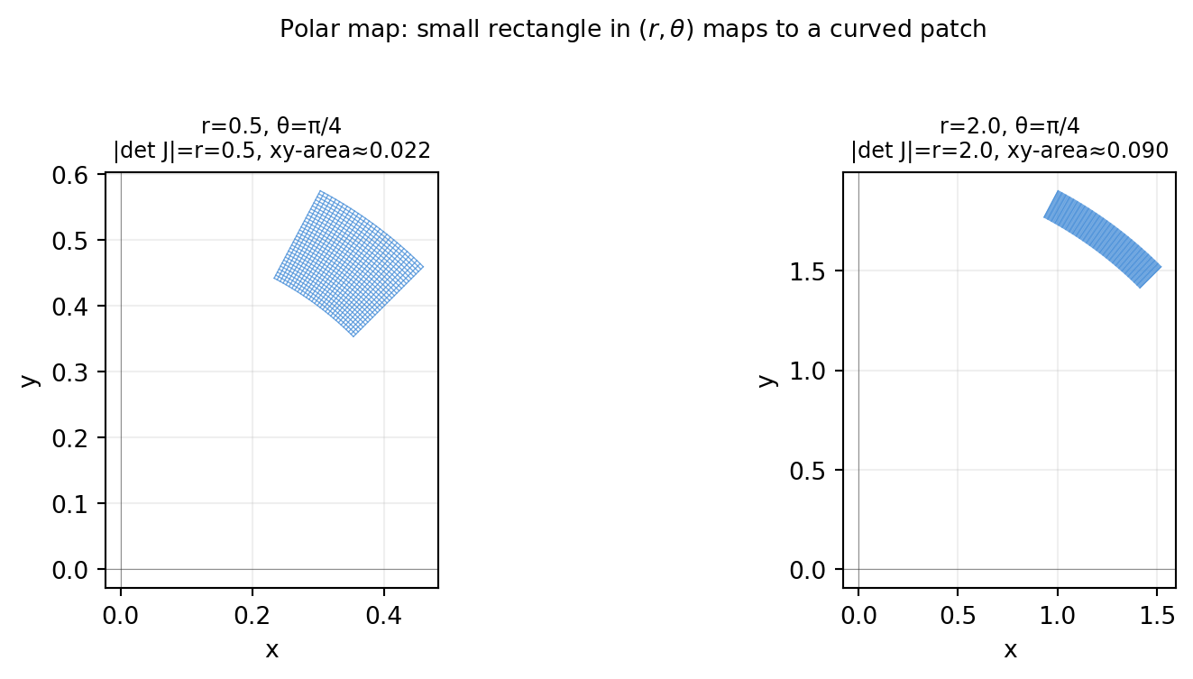
12.3.6 Jacobian Determinant: Local Area Scaling

For a differentiable map $\mathbf{f}: \mathbb{R}^n \to \mathbb{R}^n$, the Jacobian matrix $J_\mathbf{f}(\mathbf{x})$ describes the linear approximation at $\mathbf{x}$. Its determinant $|\det J_\mathbf{f}(\mathbf{x})|$ gives the local volume scaling factor:

\[\text{(volume of } \mathbf{f}(S)\text{)} \;\approx\; |\det J_\mathbf{f}(\mathbf{x})| \cdot \text{(volume of } S\text{)}\]

for small regions $S$ near $\mathbf{x}$.

This is the change-of-variables formula in integration:

\[\int_{\mathbf{f}(\Omega)} g(\mathbf{y})\,d\mathbf{y} = \int_\Omega g(\mathbf{f}(\mathbf{x}))\,|\det J_\mathbf{f}(\mathbf{x})|\,d\mathbf{x}.\]

Canonical example: polar coordinates. $\mathbf{f}(r, \theta) = (r\cos\theta,\, r\sin\theta)$.

\[J = \begin{bmatrix}\cos\theta & -r\sin\theta \\ \sin\theta & r\cos\theta\end{bmatrix}, \qquad \det J = r.\]

The familiar $r\,dr\,d\theta$ factor in polar integration is literally this Jacobian determinant.

import numpy as np
import matplotlib.pyplot as plt

# Visualise local area scaling of polar map at two points
fig, axes = plt.subplots(1, 2, figsize=(9, 3.8))

for ax, (r0, th0) in zip(axes, [(0.5, np.pi/4), (2.0, np.pi/4)]):
    dr, dth = 0.15, 0.3

    # Grid in (r, theta) space — a small square
    r_vals  = np.linspace(r0, r0 + dr, 30)
    th_vals = np.linspace(th0, th0 + dth, 30)
    R, TH   = np.meshgrid(r_vals, th_vals)
    X = R * np.cos(TH); Y = R * np.sin(TH)

    ax.plot(X, Y, color='#4a90d9', lw=0.5, alpha=0.8)
    ax.plot(X.T, Y.T, color='#4a90d9', lw=0.5, alpha=0.8)

    jac = r0   # |det J| = r
    area_param = dr * dth
    area_xy    = jac * area_param
    ax.set_title(f'r={r0}, θ=π/4\n|det J|=r={r0:.1f}, xy-area≈{area_xy:.3f}',
                 fontsize=9)
    ax.axhline(0, color='#333333', lw=0.4, alpha=0.5)
    ax.axvline(0, color='#333333', lw=0.4, alpha=0.5)
    ax.set_aspect('equal'); ax.grid(True, alpha=0.2)
    ax.set_xlabel('x'); ax.set_ylabel('y')

plt.suptitle('Polar map: small rectangle in $(r,\\theta)$ maps to a curved patch',
             fontsize=10, y=1.02)
plt.tight_layout()
plt.show()

The patch at $r=0.5$ is small; at $r=2$ the same $dr\times d\theta$ rectangle maps to a much larger area — exactly the factor $r$.

In robotics, the Jacobian determinant of a forward-kinematics map tells you where the robot is near a kinematic singularity: $\det J = 0$ means the end-effector loses a degree of freedom at that configuration.

12.3.7 Exercises

12.3.1 Verify $\det(AB) = \det(A)\det(B)$ for two random $3\times3$ matrices. Then argue geometrically: if $A$ scales volume by $\det A$ and $B$ by $\det B$, why must the composition scale by $\det(A)\det(B)$?

12.3.2 A $3\times3$ rotation $R$ has $\det(R)=+1$. Someone gives you a matrix with $\det = -1$ and claims it’s a rotation. What is it, and can it represent a physical rigid-body rotation?

12.3.3 Use cofactor_det and np.linalg.det to solve a $6\times6$ random system. Time both. How many times slower is cofactor expansion?

12.3.4 The map $(x, y) \mapsto (x^2, y^2)$ from $\mathbb{R}^2_{>0}$ to itself has Jacobian $J = \text{diag}(2x, 2y)$. Where is $|\det J| = 0$? What does that mean geometrically?

12.3.5 For a diagonal matrix $D = \text{diag}(d_1, \ldots, d_n)$, what is $\det D$? Use the signed-volume interpretation to explain why.

12.4 Condition Number and Numerical Stability

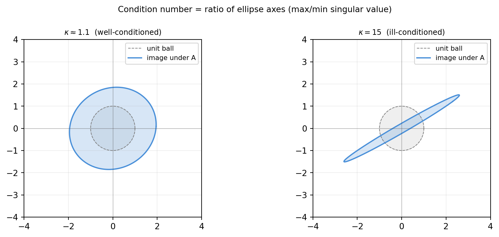
Every numerical solver ultimately operates in floating-point arithmetic, which introduces tiny rounding errors at every operation. Usually those errors are harmless — float64 carries about 16 significant digits, which is far more than any physical measurement. But some linear systems amplify rounding errors catastrophically, turning 16 correct digits of input into 4 correct digits of output. The condition number tells you exactly how bad that amplification can be.

12.4.1 Setup: Perturbations in the Right-Hand Side

Suppose we solve $A\mathbf{x} = \mathbf{b}$ and get $\mathbf{x}$, but the true right-hand side is $\mathbf{b} + \delta\mathbf{b}$ (measurement noise, rounding, numerical residual). The true solution differs by $\delta\mathbf{x}$ where $A(\delta\mathbf{x}) = \delta\mathbf{b}$, i.e., $\delta\mathbf{x} = A^{-1}\delta\mathbf{b}$.

How large can $\delta\mathbf{x}$ be relative to $\mathbf{x}$?

\[\frac{\|\delta\mathbf{x}\|}{\|\mathbf{x}\|} \;\le\; \|A\|\,\|A^{-1}\|\,\frac{\|\delta\mathbf{b}\|}{\|\mathbf{b}\|}.\]

The factor $\|A\|\,\|A^{-1}\|$ is the condition number:

\[\kappa(A) \;=\; \|A\|_2\,\|A^{-1}\|_2 \;=\; \frac{\sigma_{\max}}{\sigma_{\min}}.\]

Here $\sigma_{\max}$ and $\sigma_{\min}$ are the largest and smallest singular values of $A$. The condition number is always $\ge 1$, and $\kappa(I) = 1$ (the best possible).

12.4.2 Geometric Intuition

Think of $A$ as a linear map. It stretches space by at most $\sigma_{\max}$ in one direction and squashes it by $\sigma_{\min}$ in another. Solving $A\mathbf{x}=\mathbf{b}$ means inverting that map. A perturbation in $\mathbf{b}$ that happens to point in the most squashed direction (the direction $A$ nearly sends to zero) will be amplified by $1/\sigma_{\min}$ when inverted. The ratio $\sigma_{\max}/\sigma_{\min}$ captures the worst-case mismatch between the forward and inverse stretching.

import numpy as np
import matplotlib.pyplot as plt

fig, axes = plt.subplots(1, 2, figsize=(10, 4))

for ax, (s1, s2, title) in zip(axes, [
        (2.0, 1.8, r'$\kappa \approx 1.1$  (well-conditioned)'),
        (3.0, 0.2, r'$\kappa = 15$  (ill-conditioned)')]):

    theta = np.linspace(0, 2 * np.pi, 300)
    circle = np.stack([np.cos(theta), np.sin(theta)])   # shape (2, 300)

    # Rotate 30 degrees
    c30, s30 = np.cos(np.pi / 6), np.sin(np.pi / 6)
    R = np.array([[c30, -s30], [s30, c30]])
    A = R @ np.diag([s1, s2]) @ R.T

    ellipse = A @ circle   # shape (2, 300)

    ax.fill(circle[0], circle[1], alpha=0.12, color='gray')
    ax.plot(circle[0], circle[1], '--', color='gray', lw=0.8, label='unit ball')
    ax.fill(ellipse[0], ellipse[1], alpha=0.22, color='#4a90d9')
    ax.plot(ellipse[0], ellipse[1], '-', color='#4a90d9', lw=1.5, label='image under A')
    ax.axhline(0, color='#333333', lw=0.4, alpha=0.5)
    ax.axvline(0, color='#333333', lw=0.4, alpha=0.5)
    ax.set_aspect('equal')
    ax.set_xlim(-4, 4); ax.set_ylim(-4, 4)
    ax.grid(True, alpha=0.2)
    ax.set_title(title, fontsize=9)
    ax.legend(fontsize=8)

plt.suptitle('Condition number = ratio of ellipse axes (max/min singular value)',
             fontsize=10)
plt.tight_layout()
plt.show()

12.4.3 The Digit-Loss Rule

Floating-point arithmetic introduces relative rounding errors of order $\varepsilon_{\text{machine}}$:

Precision	$\varepsilon_{\text{machine}}$	Decimal digits
float32	$\approx 1.19 \times 10^{-7}$	~7
float64	$\approx 2.22 \times 10^{-16}$	~16

After solving $A\mathbf{x}=\mathbf{b}$ in floating-point, the relative error in $\mathbf{x}$ is roughly:

\[\frac{\|\mathbf{x}_{\text{computed}} - \mathbf{x}_{\text{true}}\|}{\|\mathbf{x}_{\text{true}}\|} \;\approx\; \kappa(A)\,\varepsilon_{\text{machine}}.\]

So you lose approximately $\log_{10}\kappa(A)$ digits of accuracy.

Examples:

$\kappa = 10^4$, float64: $16 - 4 = 12$ correct digits. Fine.
$\kappa = 10^{10}$, float64: $16 - 10 = 6$ correct digits. Acceptable for most applications.
$\kappa = 10^{10}$, float32: $7 - 10 = -3$ — negative — meaning the answer is noise.
$\kappa = 10^{14}$, float64: only 2 reliable digits. Switch to higher precision or reformulate.

import numpy as np
import matplotlib.pyplot as plt

rng = np.random.default_rng(23)

def hilbert(n):
    """Hilbert matrix — famously ill-conditioned."""
    i, j = np.meshgrid(np.arange(1, n+1), np.arange(1, n+1))
    return 1.0 / (i + j - 1)   # shape (n, n)

ns = range(2, 14)
kappas, errs64, errs32 = [], [], []

for n in ns:
    A = hilbert(n)                  # shape (n, n)
    x_true = np.ones(n)            # shape (n,)
    b = A @ x_true                 # shape (n,)

    x64 = np.linalg.solve(A.astype(np.float64), b.astype(np.float64))
    x32 = np.linalg.solve(A.astype(np.float32), b.astype(np.float32)).astype(np.float64)

    kappas.append(np.linalg.cond(A))
    errs64.append(np.linalg.norm(x64 - x_true) / np.linalg.norm(x_true) + 1e-20)
    errs32.append(np.linalg.norm(x32 - x_true) / np.linalg.norm(x_true) + 1e-20)

kappas = np.array(kappas)
errs64 = np.array(errs64)
errs32 = np.array(errs32)

fig, ax = plt.subplots(figsize=(7, 4.5))
ax.loglog(kappas, errs64, 'o-', color='#4a90d9', lw=1.5, label='float64')
ax.loglog(kappas, errs32, 's-', color='tomato',  lw=1.5, label='float32')

# Reference lines: kappa * eps
eps64 = np.finfo(np.float64).eps
eps32 = np.finfo(np.float32).eps
ax.loglog(kappas, kappas * eps64, '--', color='#4a90d9', lw=0.8, alpha=0.6, label=r'$\kappa\,\varepsilon_{64}$')
ax.loglog(kappas, kappas * eps32, '--', color='tomato',  lw=0.8, alpha=0.6, label=r'$\kappa\,\varepsilon_{32}$')

ax.set_xlabel(r'condition number  $\kappa(A)$')
ax.set_ylabel('relative error in solution')
ax.set_title('Digit loss: Hilbert matrix solve in float32 vs float64', fontsize=10)
ax.axhline(1.0, color='black', lw=0.5, alpha=0.4, linestyle=':')
ax.grid(True, which='both', alpha=0.2)
ax.legend(fontsize=9)
plt.tight_layout()
plt.show()

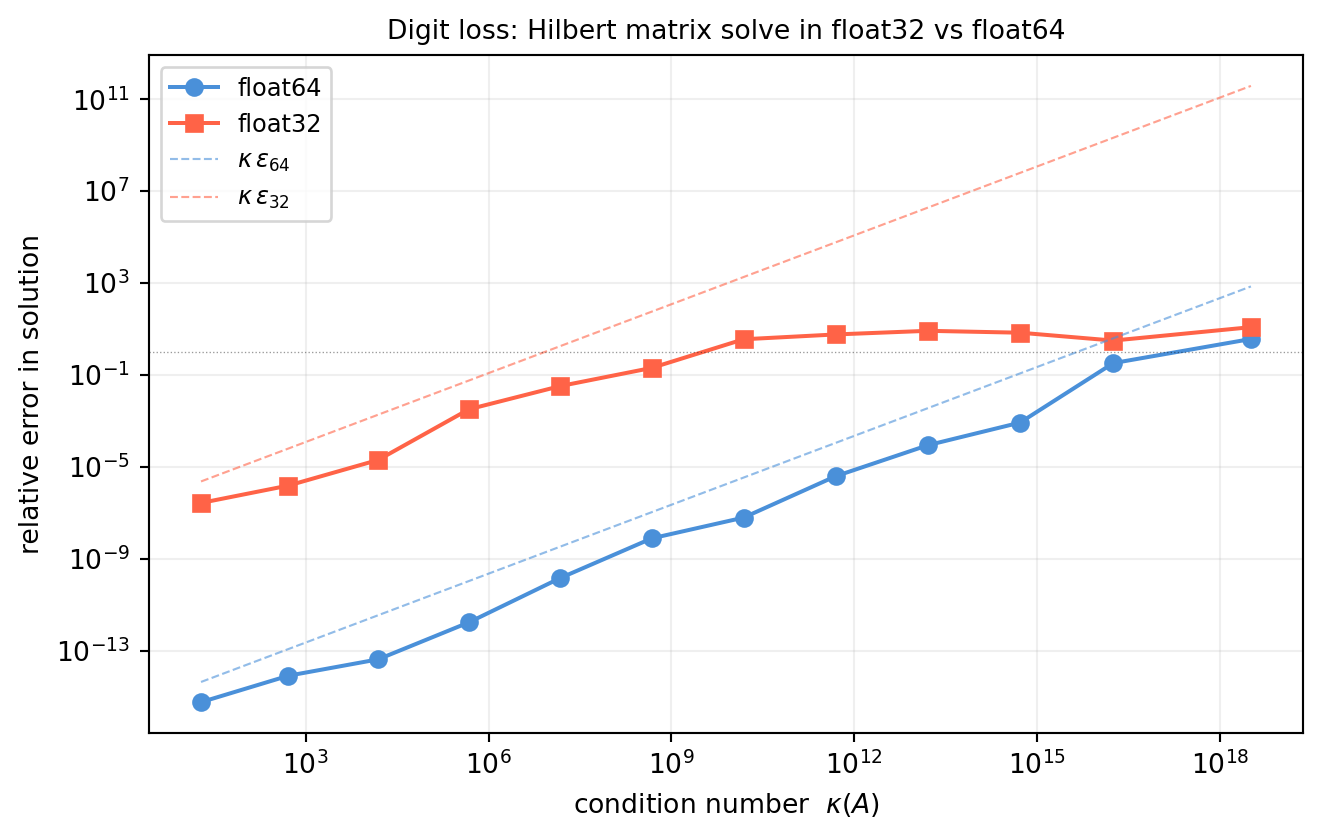
Notice how the float32 curve hits 1.0 (completely wrong answer) once $\kappa \gtrsim 10^7$, while float64 stays reliable until $\kappa \approx 10^{14}$.

12.4.4 Why Camera Calibration Is Notoriously Ill-Conditioned

The intrinsic matrix $K$ from Chapter 10 has entries on vastly different scales:

\[K = \begin{bmatrix} f_x & 0 & c_x \\ 0 & f_y & c_y \\ 0 & 0 & 1 \end{bmatrix}, \qquad f_x, f_y \sim 1000\text{ px}, \quad c_x, c_y \sim 500\text{ px}, \quad K_{33} = 1.\]

The ratio between the largest and smallest entries is about $10^3$. The DLT calibration system (Chapter 10) assembles a matrix whose columns mix these scales. Without normalization the condition number is $\kappa \sim 10^6$–$10^8$, consuming 6–8 digits of float64 precision.

This is why Zhang’s method normalizes image coordinates before assembling the DLT system — it brings $\kappa$ down by several orders of magnitude.

import numpy as np

# Simulate a poorly-scaled 3x3 system like an unnormalized DLT subblock
# K-matrix scale mismatch
K = np.array([[1200.,    0., 640.],
              [   0., 1200., 480.],
              [   0.,    0.,   1.]])   # shape (3, 3)

print("Condition number of K:", np.linalg.cond(K).round(1))

# After dividing by image size ~ 1000 (rough normalization)
scale = 1000.
K_norm = K / scale
K_norm[2, 2] = 1.   # keep the homogeneous entry
print("Condition number of K (normalized):", np.linalg.cond(K_norm).round(1))

Condition number of K: 1733.3
Condition number of K (normalized): 2.1

12.4.5 When to Use float32 vs float64

Situation	Recommendation
$\kappa \lesssim 10^4$, GPU inference	float32 safe (gains ~2× throughput)
Stochastic gradient descent	float32 fine (noise dominates anyway)
$\kappa \sim 10^6$–$10^9$	float64 preferred
Camera calibration, SLAM	float64 (ill-conditioned by nature)
$\kappa > 10^{12}$	Reformulate, precondition, or use higher precision

The rough rule: if the condition number times the machine epsilon exceeds your acceptable error tolerance, switch to higher precision or reformulate the problem.

12.4.6 Computing the Condition Number

import numpy as np

rng = np.random.default_rng(29)
A = rng.standard_normal((5, 5))   # shape (5, 5)

# Full condition number (ratio of singular values)
kappa = np.linalg.cond(A)
print(f"kappa(A)             = {kappa:.4f}")

# Via SVD directly
sigma = np.linalg.svd(A, compute_uv=False)   # shape (5,)
print(f"sigma_max / sigma_min = {sigma[0] / sigma[-1]:.4f}")

# Singular matrix: infinite condition number
A_sing = A.copy(); A_sing[:, 4] = A_sing[:, 3]   # make rank-4
print(f"\nkappa(singular A) = {np.linalg.cond(A_sing):.3e}")

kappa(A)             = 18.3083
sigma_max / sigma_min = 18.3083

kappa(singular A) = 2.852e+17

For a singular matrix $\sigma_{\min} = 0$ so $\kappa = \infty$ — confirmed by the large number above (numpy returns a large finite value limited by float64 precision).

12.4.7 Exercises

12.4.1 What is $\kappa(I_n)$? What is $\kappa(R)$ for any orthogonal $R$? Why do rotations cause zero digit loss?

12.4.2 Can $\kappa(A) < 1$? Prove it from the definition $\kappa = \sigma_{\max}/\sigma_{\min}$.

12.4.3 If $\kappa(A) = 10^{10}$, how many digits of the solution are reliable in float32? In float64? What if $\kappa = 10^{6}$?

12.4.4 np.linalg.cond(A) calls SVD internally ($O(n^3)$). Suppose you have already computed the Cholesky factor $L$ of a symmetric PD matrix $A$. Can you estimate $\kappa(A)$ from $L$ without a full SVD? (Hint: LAPACK’s dpotri offers a cheap reciprocal-condition-number estimator.)

12.4.5 Build a $10\times10$ Hilbert matrix. Solve $A\mathbf{x}=\mathbf{b}$ with $\mathbf{b} = A\mathbf{1}$ in float32 and float64. How many digits agree with the true solution $\mathbf{x}=\mathbf{1}$? Does the prediction from $\kappa \varepsilon_{\text{machine}}$ match the observed error?

12.5 Sparse Matrices: Formats and Solvers

The systems we have factorized so far assume that every entry of $A$ is potentially nonzero — a dense matrix. But many of the largest linear systems in ML/CV/robotics are almost entirely zero:

SLAM factor graph. A pose graph with 10,000 poses has a Hessian $H \in \mathbb{R}^{30000\times30000}$ (3 DOF per pose). Storing it as dense requires $$7 GB. But each pose connects to only a handful of neighbors, so $H$ has roughly $10^5$ nonzeros out of $9\times10^8$ entries — a fill fraction of 0.01 %.
Bundle adjustment. The Jacobian of $m$ observations over $n$ 3D points and $k$ cameras is $(2m)\times(3n+6k)$. Each row has nonzeros in only one camera block and one point block — 9 nonzeros out of perhaps $10^6$ columns.
FEM / PDE solvers. Discretizing a PDE on a mesh connects each node to its neighbors. The stiffness matrix is banded.

Exploiting sparsity is the difference between solving a problem in seconds and it being computationally infeasible.

12.5.1 Storage Formats

Three formats cover essentially all use cases.

12.5.1.1 COO — Coordinate Format

Three arrays: row, col, data — one triple $(i, j, v)$ per nonzero. Simple to build, but slow for arithmetic.

12.5.1.2 CSR — Compressed Sparse Row

Three arrays: - data[k]: the $k$-th nonzero value. - indices[k]: the column index of data[k]. - indptr[i]: offset in data where row $i$ begins; indptr[i+1] is where it ends.

Row $i$ has nonzeros at columns indices[indptr[i]:indptr[i+1]] with values data[indptr[i]:indptr[i+1]].

CSR supports fast $y = Ax$ (iterate over rows) and is the default for general sparse operations.

12.5.1.3 CSC — Compressed Sparse Column

The column-oriented transpose of CSR. Fast for $y = A^Tx$ and column operations. Most sparse direct solvers (CHOLMOD, SuperLU) prefer CSC input.

import numpy as np
import scipy.sparse as sp

# Build a small sparse matrix in COO, then convert
row  = np.array([0, 0, 1, 2, 2])
col  = np.array([0, 2, 1, 0, 2])
data = np.array([3., 1., 4., 1., 5.])

A_coo = sp.coo_matrix((data, (row, col)), shape=(3, 3))
A_csr = A_coo.tocsr()
A_csc = A_coo.tocsc()

print("Dense:\n", A_coo.toarray())
print("\nCSR indptr  :", A_csr.indptr)
print("CSR indices :", A_csr.indices)
print("CSR data    :", A_csr.data)
print("\nnnz (nonzeros):", A_csr.nnz, "out of", 3*3)

Dense:
 [[3. 0. 1.]
 [0. 4. 0.]
 [1. 0. 5.]]

CSR indptr  : [0 2 3 5]
CSR indices : [0 2 1 0 2]
CSR data    : [3. 1. 4. 1. 5.]

nnz (nonzeros): 5 out of 9

Rule of thumb: build in COO (easy to assemble), convert to CSR/CSC for factorization and matrix-vector products.

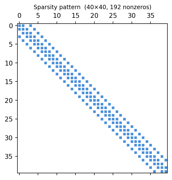
12.5.2 Sparsity Patterns: Visualizing with `spy`

import numpy as np
import scipy.sparse as sp
import matplotlib.pyplot as plt

rng = np.random.default_rng(31)
n = 40

# Banded SPD matrix: tridiagonal + some off-diagonal connections
diags = [4*np.ones(n), -np.ones(n-1), -np.ones(n-1),
         0.5*np.ones(n-3), 0.5*np.ones(n-3)]
offsets = [0, 1, -1, 3, -3]
A = sp.diags(diags, offsets, shape=(n, n), format='csr')
A = A + A.T                               # make symmetric
# ensure diagonal dominance (ravel avoids numpy.matrix from .diagonal())
d = np.asarray(A.diagonal()).ravel()
A = A + sp.diags(4 - d)

fig, ax = plt.subplots(figsize=(4, 4))
ax.spy(np.asarray(A.todense()), markersize=3, color='#4a90d9')
ax.set_title(f'Sparsity pattern  ({n}×{n}, {A.nnz} nonzeros)', fontsize=9)
plt.tight_layout()
plt.show()

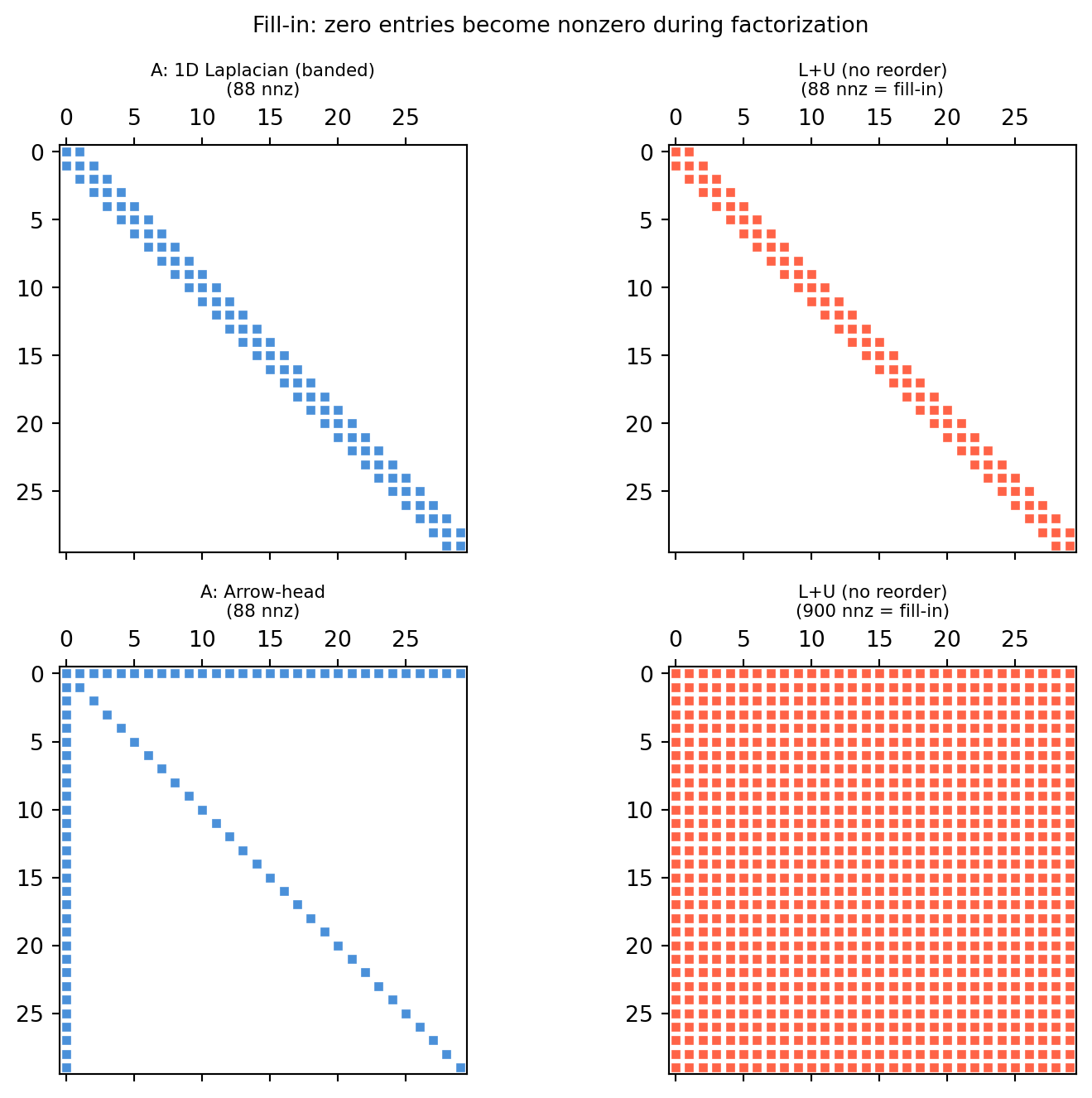
12.5.3 Fill-In: Why Sparsity Doesn’t Survive Naive Factorization

When you factorize a sparse matrix with Gaussian elimination, a zero entry $a_{ij}=0$ can become nonzero in $L$ or $U$ — a fill-in. In the worst case (e.g., an arrow-head matrix) the factor is completely dense even though the original matrix was $O(n)$ nonzeros.

import numpy as np
import scipy.sparse as sp
from scipy.sparse.linalg import splu
import matplotlib.pyplot as plt

n = 30

# 1D Laplacian: banded, O(n) nonzeros
diag_main = 2.0 * np.ones(n)
diag_off  = -1.0 * np.ones(n - 1)
A_lap = sp.diags([diag_main, diag_off, diag_off],
                 [0, 1, -1], format='csc')

# Arrow-head: diagonal + first row/col (star graph)
rows = np.concatenate([[0]*n, np.arange(1, n), np.arange(n)])
cols = np.concatenate([np.arange(n), np.zeros(n-1, int), np.arange(n)])
vals = np.concatenate([np.ones(n), np.ones(n-1), np.ones(n-1), np.ones(n)])
A_arrow = sp.csc_matrix((np.ones(len(rows)), (rows, cols)),
                         shape=(n, n))
A_arrow = A_arrow + A_arrow.T
A_arrow.setdiag(A_arrow.diagonal() + n)   # make diagonally dominant

fig, axes = plt.subplots(2, 2, figsize=(8, 7))

for ax_orig, ax_factor, A, title in zip(
        [axes[0, 0], axes[1, 0]],
        [axes[0, 1], axes[1, 1]],
        [A_lap,      A_arrow],
        ['1D Laplacian (banded)', 'Arrow-head']):

    lu_obj = splu(A, permc_spec='NATURAL')
    L_dense = lu_obj.L.toarray()
    U_dense = lu_obj.U.toarray()
    LU_combined = np.abs(L_dense) + np.abs(U_dense)

    ax_orig.spy(A.toarray(), markersize=3, color='#4a90d9')
    ax_orig.set_title(f'A: {title}\n({A.nnz} nnz)', fontsize=8)

    ax_factor.spy(LU_combined > 1e-12, markersize=3, color='tomato')
    nnz_lu = int(np.sum(LU_combined > 1e-12))
    ax_factor.set_title(f'L+U (no reorder)\n({nnz_lu} nnz = fill-in)', fontsize=8)

plt.suptitle('Fill-in: zero entries become nonzero during factorization', fontsize=10)
plt.tight_layout()
plt.show()

The banded Laplacian stays banded in $L+U$: fill-in is local. The arrow-head is catastrophic: every entry of $L$ is nonzero because the first row/column connects every node to every other.

12.5.4 Reordering: Minimizing Fill-In

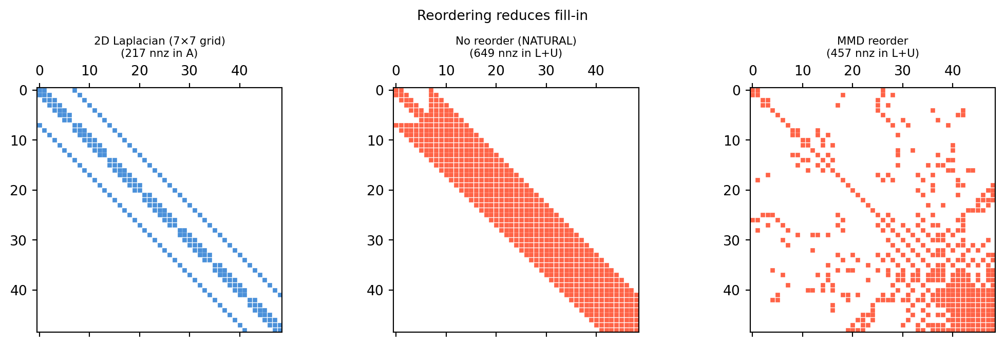
The key insight: reordering rows and columns of $A$ (with the same permutation on both sides for symmetric $A$) doesn’t change the solution, but can dramatically reduce fill-in in $L$.

Formally, for symmetric $A$ we seek permutation $P$ such that $L$ in $PAP^T = LL^T$ is as sparse as possible. Finding the optimal $P$ is NP-hard, but two heuristics work very well in practice:

AMD (Approximate Minimum Degree). Greedily eliminates the variable that currently has the fewest connections in the remaining graph. Available as scipy.sparse.csgraph.minimum_degree_ordering or scikit-sparse.
METIS (Nested Dissection). Recursively finds a small separator of the graph — nodes whose removal splits the graph in two — and eliminates interior nodes before the separator. Exceptional for mesh/graph-like sparsity (SLAM, FEM).

import numpy as np
import scipy.sparse as sp
from scipy.sparse.linalg import splu
import matplotlib.pyplot as plt

n = 50

# 2D Laplacian on n/5 x n/5 grid (unstructured but grid-like)
# Build manually: each interior node connected to 4 neighbors
side = int(n**0.5)
N = side * side
rows, cols, vals = [], [], []
for i in range(side):
    for j in range(side):
        idx = i * side + j
        rows.append(idx); cols.append(idx); vals.append(4.)
        for di, dj in [(-1,0),(1,0),(0,-1),(0,1)]:
            ni, nj = i+di, j+dj
            if 0 <= ni < side and 0 <= nj < side:
                rows.append(idx); cols.append(ni*side+nj); vals.append(-1.)
A2d = sp.csc_matrix((vals, (rows, cols)), shape=(N, N))

fig, axes = plt.subplots(1, 3, figsize=(11, 3.5))

lu_nat = splu(A2d, permc_spec='NATURAL')
lu_mmd = splu(A2d, permc_spec='MMD_AT_PLUS_A')   # min-degree reordering

for ax, lu_obj, title in zip(axes[1:],
                              [lu_nat, lu_mmd],
                              ['No reorder (NATURAL)', 'MMD reorder']):
    L = lu_obj.L.toarray(); U = lu_obj.U.toarray()
    combo = np.abs(L) + np.abs(U)
    ax.spy(combo > 1e-12, markersize=2, color='tomato')
    nnz = int(np.sum(combo > 1e-12))
    ax.set_title(f'{title}\n({nnz} nnz in L+U)', fontsize=8)

axes[0].spy(A2d.toarray(), markersize=2, color='#4a90d9')
axes[0].set_title(f'2D Laplacian ({side}×{side} grid)\n({A2d.nnz} nnz in A)', fontsize=8)
plt.suptitle('Reordering reduces fill-in', fontsize=10)
plt.tight_layout()
plt.show()

12.5.5 Sparse Solvers in SciPy

# Direct sparse solve (SuperLU under the hood)
from scipy.sparse.linalg import spsolve
x = spsolve(A, b)

# Pre-factor for multiple right-hand sides
from scipy.sparse.linalg import factorized
solve = factorized(A)   # returns a callable
x1 = solve(b1)
x2 = solve(b2)

# Iterative: Conjugate Gradient (SPD systems only)
from scipy.sparse.linalg import cg
x, info = cg(A, b, tol=1e-10)

# Iterative: GMRES (general systems)
from scipy.sparse.linalg import gmres
x, info = gmres(A, b, tol=1e-10)

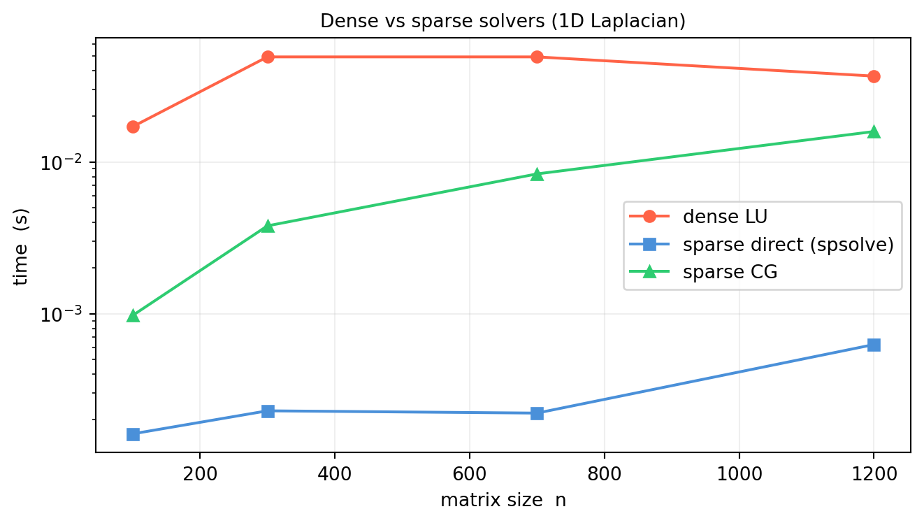
import numpy as np
import scipy.sparse as sp
from scipy.sparse.linalg import spsolve, cg
import time

rng = np.random.default_rng(37)
ns = [100, 300, 700, 1200]
t_dense, t_sparse, t_cg = [], [], []

for n in ns:
    # 1D Laplacian (tridiagonal SPD)
    main  = 2. * np.ones(n)
    off   = -1. * np.ones(n - 1)
    A_sp  = sp.diags([main, off, off], [0, 1, -1], format='csc')
    A_den = A_sp.toarray()
    b     = rng.standard_normal(n)   # shape (n,)

    t0 = time.perf_counter()
    np.linalg.solve(A_den, b)
    t_dense.append(time.perf_counter() - t0)

    t0 = time.perf_counter()
    spsolve(A_sp, b)
    t_sparse.append(time.perf_counter() - t0)

    t0 = time.perf_counter()
    cg(A_sp, b, rtol=1e-10)
    t_cg.append(time.perf_counter() - t0)

import matplotlib.pyplot as plt
fig, ax = plt.subplots(figsize=(7, 4))
ax.semilogy(ns, t_dense,  'o-', color='tomato',   lw=1.5, label='dense LU')
ax.semilogy(ns, t_sparse, 's-', color='#4a90d9',  lw=1.5, label='sparse direct (spsolve)')
ax.semilogy(ns, t_cg,     '^-', color='#2ecc71',  lw=1.5, label='sparse CG')
ax.set_xlabel('matrix size  n')
ax.set_ylabel('time  (s)')
ax.set_title('Dense vs sparse solvers (1D Laplacian)', fontsize=10)
ax.grid(True, alpha=0.2)
ax.legend()
plt.tight_layout()
plt.show()

For the banded Laplacian, sparse direct is orders of magnitude faster than dense LU — which spends $O(n^3)$ on operations that are already zero in $A$.

12.5.6 When to Use Each Solver

System	Solver
Dense, general	LU (`np.linalg.solve`)
Dense, SPD	Cholesky (`scipy.linalg.cho_factor`)
Sparse, general	`spsolve` (direct) or GMRES (iterative)
Sparse, SPD, many RHS	`factorized` or sparse Cholesky (CHOLMOD)
Extremely large, SPD	Conjugate Gradient with preconditioner
Sparse but very large + memory-limited	MINRES / LSQR

Iterative solvers (CG, GMRES) avoid storing the factor entirely, which matters when the factor would be much denser than $A$ even with reordering.

12.5.7 Exercises

12.5.1 Why doesn’t row/column reordering change the solution? Give a one-sentence proof.

12.5.2 Is spsolve faster than np.linalg.solve for a dense matrix stored as a scipy sparse matrix? Try it. What overhead does sparse format add for dense problems?

12.5.3 An arrow-head matrix has nonzeros only on the diagonal and in the first row/column. Its LU without reordering is completely dense (as demonstrated above). What reordering eliminates all fill-in? (Hint: which variable should you eliminate last?)

12.5.4 When should you prefer an iterative solver (CG) over a direct sparse solver (spsolve)? Name two concrete criteria.

12.5.5 Build a random sparse matrix with 5% fill by zeroing out entries of a dense random matrix, then convert to CSR. Time both np.linalg.solve (dense) and spsolve (sparse). At what fill percentage does the crossover happen?

12.6 Application: Sparse Cholesky for Factor Graph Optimization

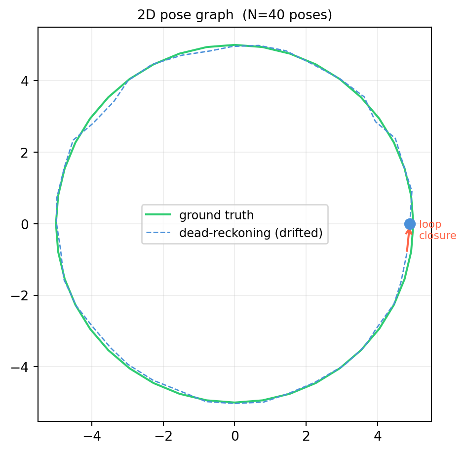
Factor graph optimization is the backbone of modern SLAM (Simultaneous Localization and Mapping). A robot navigates a loop, accumulates odometry errors, and later recognizes a previously-visited place — a loop closure — which allows it to distribute the accumulated error across the entire trajectory.

The optimization problem is a nonlinear least squares over robot poses. After linearization (Gauss-Newton step), it becomes a large linear system whose coefficient matrix is sparse and symmetric positive-definite. This is exactly where sparse Cholesky earns its keep.

12.6.1 The 2D Pose Graph Model

A 2D pose is a triple $(x, y, \theta)$. We simulate $N$ poses arranged in a noisy ring:

Odometry factors constrain consecutive poses: pose $i$ and pose $i+1$ are connected.
Loop closure factor constrains pose $0$ and pose $N-1$: the robot has returned to its start.

Each factor contributes a block to the Hessian $H = J^T \Omega J$ (the normal equations of the nonlinear least squares). The structure of $H$ is:

Block-tridiagonal from the odometry chain (each pose $i$ connects to pose $i+1$).
One corner block $(0, N-1)$ from the loop closure.

import numpy as np
import matplotlib.pyplot as plt

rng = np.random.default_rng(41)
N = 40  # number of poses

# Ground truth: evenly spaced around a circle of radius 5
theta_gt = np.linspace(0, 2 * np.pi, N, endpoint=False)
x_gt = 5. * np.cos(theta_gt)   # shape (N,)
y_gt = 5. * np.sin(theta_gt)   # shape (N,)

# Noisy estimated trajectory (dead-reckoning drift)
noise_xy = 0.08
noise_th = 0.04
x_est = x_gt + rng.standard_normal(N) * noise_xy   # shape (N,)
y_est = y_gt + rng.standard_normal(N) * noise_xy   # shape (N,)

fig, ax = plt.subplots(figsize=(5, 5))
ax.plot(np.append(x_gt, x_gt[0]), np.append(y_gt, y_gt[0]),
        '-', color='#2ecc71', lw=1.5, label='ground truth')
ax.plot(np.append(x_est, x_est[0]), np.append(y_est, y_est[0]),
        '--', color='#4a90d9', lw=1.0, label='dead-reckoning (drifted)')

# Mark loop closure
ax.annotate('', xy=(x_est[0], y_est[0]), xytext=(x_est[-1], y_est[-1]),
            arrowprops=dict(arrowstyle='->', color='tomato', lw=1.5))
ax.text((x_est[0]+x_est[-1])/2 + 0.3, (y_est[0]+y_est[-1])/2,
        'loop\nclosure', color='tomato', fontsize=8)

ax.scatter(x_est[0], y_est[0], s=60, color='#4a90d9', zorder=5)
ax.set_aspect('equal'); ax.grid(True, alpha=0.2)
ax.legend(fontsize=9)
ax.set_title(f'2D pose graph  (N={N} poses)', fontsize=10)
plt.tight_layout()
plt.show()

12.6.2 Building the Hessian $H$

Each pose has 2 DOF (we fix orientation for clarity, treating translation only). The Hessian $H \in \mathbb{R}^{2N\times 2N}$ accumulates $2\times 2$ blocks from each factor.

Odometry factor between poses $i$ and $i+1$: contributes to blocks $(i,i)$, $(i,i+1)$, $(i+1,i)$, $(i+1,i+1)$.

Loop closure factor between poses $0$ and $N-1$: contributes to blocks $(0,0)$, $(0,N-1)$, $(N-1,0)$, $(N-1,N-1)$.

We use information matrix $\Omega = \sigma^{-2} I_2$ (isotropic Gaussian noise) for each factor.

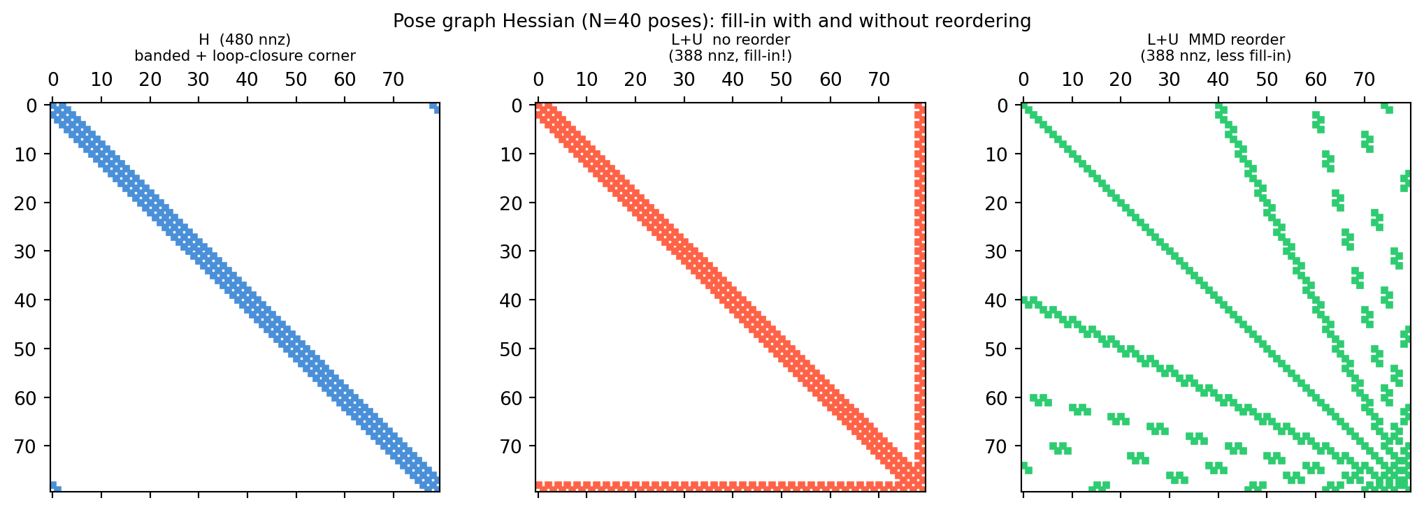
import numpy as np
import scipy.sparse as sp

def build_pose_graph_hessian(N, sigma_odom=0.1, sigma_loop=0.05):
    """
    Build the Hessian of a 2D pose-graph with:
      - N-1 odometry factors (consecutive poses)
      - 1 loop-closure factor (pose 0 <-> pose N-1)
    Pose DOF: 2 (x, y). Total size: 2N x 2N.
    Returns scipy CSC sparse matrix.
    """
    dof = 2
    size = N * dof
    rows, cols, vals = [], [], []

    def add_block(i, j, B):
        """Add 2x2 block B at block position (i,j)."""
        for di in range(dof):
            for dj in range(dof):
                rows.append(i * dof + di)
                cols.append(j * dof + dj)
                vals.append(B[di, dj])

    Omega_odom = np.eye(dof) / sigma_odom**2   # shape (2, 2)
    Omega_loop = np.eye(dof) / sigma_loop**2   # shape (2, 2)

    # Odometry factors: poses 0..N-2 connected to 1..N-1
    for i in range(N - 1):
        add_block(i,   i,   Omega_odom)
        add_block(i+1, i+1, Omega_odom)
        add_block(i,   i+1, -Omega_odom)
        add_block(i+1, i,   -Omega_odom)

    # Loop closure: pose 0 <-> pose N-1
    add_block(0,   0,   Omega_loop)
    add_block(N-1, N-1, Omega_loop)
    add_block(0,   N-1, -Omega_loop)
    add_block(N-1, 0,   -Omega_loop)

    # Anchor pose 0 to fix gauge freedom (global translation unobservable)
    add_block(0, 0, np.eye(dof) * 1e6)

    H = sp.csc_matrix((vals, (rows, cols)), shape=(size, size))
    # Symmetrize (accumulated duplicate entries are summed by csc_matrix)
    return H

N = 40
H = build_pose_graph_hessian(N)
print(f"H size    : {H.shape[0]} × {H.shape[1]}")
print(f"H nnz     : {H.nnz}  ({100*H.nnz/H.shape[0]**2:.2f}% dense)")

H size    : 80 × 80
H nnz     : 480  (7.50% dense)

12.6.3 Sparsity Pattern of $H$

import numpy as np
import scipy.sparse as sp
import matplotlib.pyplot as plt

def build_pose_graph_hessian(N, sigma_odom=0.1, sigma_loop=0.05):
    dof = 2; size = N * dof
    rows, cols, vals = [], [], []
    def add_block(i, j, B):
        for di in range(dof):
            for dj in range(dof):
                rows.append(i*dof+di); cols.append(j*dof+dj); vals.append(B[di,dj])
    Omega_odom = np.eye(dof) / sigma_odom**2
    Omega_loop = np.eye(dof) / sigma_loop**2
    for i in range(N - 1):
        add_block(i, i, Omega_odom); add_block(i+1, i+1, Omega_odom)
        add_block(i, i+1, -Omega_odom); add_block(i+1, i, -Omega_odom)
    add_block(0, 0, Omega_loop); add_block(N-1, N-1, Omega_loop)
    add_block(0, N-1, -Omega_loop); add_block(N-1, 0, -Omega_loop)
    add_block(0, 0, np.eye(dof) * 1e6)  # anchor pose 0 (fixes gauge freedom)
    return sp.csc_matrix((vals, (rows, cols)), shape=(size, size))

N = 40
H = build_pose_graph_hessian(N)

fig, axes = plt.subplots(1, 3, figsize=(11, 3.8))

# Original H
axes[0].spy(H, markersize=3, color='#4a90d9')
axes[0].set_title(f'H  ({H.nnz} nnz)\nbanded + loop-closure corner', fontsize=8)

# LU without reordering
from scipy.sparse.linalg import splu
lu_nat = splu(H, permc_spec='NATURAL')
L_nat = lu_nat.L.toarray(); U_nat = lu_nat.U.toarray()
combo_nat = np.abs(L_nat) + np.abs(U_nat)
nnz_nat = int(np.sum(combo_nat > 1e-12))
axes[1].spy(combo_nat > 1e-12, markersize=3, color='tomato')
axes[1].set_title(f'L+U  no reorder\n({nnz_nat} nnz, fill-in!)', fontsize=8)

# LU with MMD reordering
lu_mmd = splu(H, permc_spec='MMD_AT_PLUS_A')
L_mmd = lu_mmd.L.toarray(); U_mmd = lu_mmd.U.toarray()
combo_mmd = np.abs(L_mmd) + np.abs(U_mmd)
nnz_mmd = int(np.sum(combo_mmd > 1e-12))
axes[2].spy(combo_mmd > 1e-12, markersize=3, color='#2ecc71')
axes[2].set_title(f'L+U  MMD reorder\n({nnz_mmd} nnz, less fill-in)', fontsize=8)

plt.suptitle(f'Pose graph Hessian (N={N} poses): fill-in with and without reordering',
             fontsize=10)
plt.tight_layout()
plt.show()

The loop-closure block in the top-right/bottom-left corners is what triggers heavy fill-in without reordering — the variable-elimination order must handle that “shortcut” edge carefully.

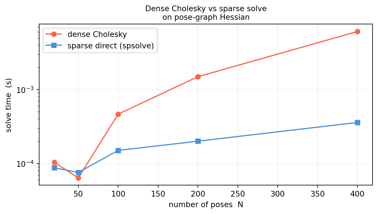
12.6.4 Dense vs Sparse Cholesky: Timing

import numpy as np
import scipy.sparse as sp
from scipy.sparse.linalg import spsolve, factorized
from scipy.linalg import cho_factor, cho_solve
import time

def build_pose_graph_hessian(N, sigma_odom=0.1, sigma_loop=0.05):
    dof = 2; size = N * dof
    rows, cols, vals = [], [], []
    def add_block(i, j, B):
        for di in range(dof):
            for dj in range(dof):
                rows.append(i*dof+di); cols.append(j*dof+dj); vals.append(B[di,dj])
    Omega_odom = np.eye(dof) / sigma_odom**2
    Omega_loop = np.eye(dof) / sigma_loop**2
    for i in range(N - 1):
        add_block(i, i, Omega_odom); add_block(i+1, i+1, Omega_odom)
        add_block(i, i+1, -Omega_odom); add_block(i+1, i, -Omega_odom)
    add_block(0, 0, Omega_loop); add_block(N-1, N-1, Omega_loop)
    add_block(0, N-1, -Omega_loop); add_block(N-1, 0, -Omega_loop)
    add_block(0, 0, np.eye(dof) * 1e6)  # anchor pose 0 (fixes gauge freedom)
    return sp.csc_matrix((vals, (rows, cols)), shape=(size, size))

rng = np.random.default_rng(43)
Ns = [20, 50, 100, 200, 400]
t_dense, t_sparse = [], []

for N in Ns:
    H = build_pose_graph_hessian(N)
    H_dense = H.toarray()
    b = rng.standard_normal(H.shape[0])   # shape (2N,)

    t0 = time.perf_counter()
    cf = cho_factor(H_dense)
    cho_solve(cf, b)
    t_dense.append(time.perf_counter() - t0)

    t0 = time.perf_counter()
    spsolve(H, b)
    t_sparse.append(time.perf_counter() - t0)

import matplotlib.pyplot as plt
fig, ax = plt.subplots(figsize=(7, 4))
ax.semilogy(Ns, t_dense,  'o-', color='tomato',  lw=1.5, label='dense Cholesky')
ax.semilogy(Ns, t_sparse, 's-', color='#4a90d9', lw=1.5, label='sparse direct (spsolve)')
ax.set_xlabel('number of poses  N')
ax.set_ylabel('solve time  (s)')
ax.set_title('Dense Cholesky vs sparse solve\non pose-graph Hessian', fontsize=10)
ax.grid(True, alpha=0.2)
ax.legend()
plt.tight_layout()
plt.show()

12.6.5 Using the Factorization to Correct the Trajectory

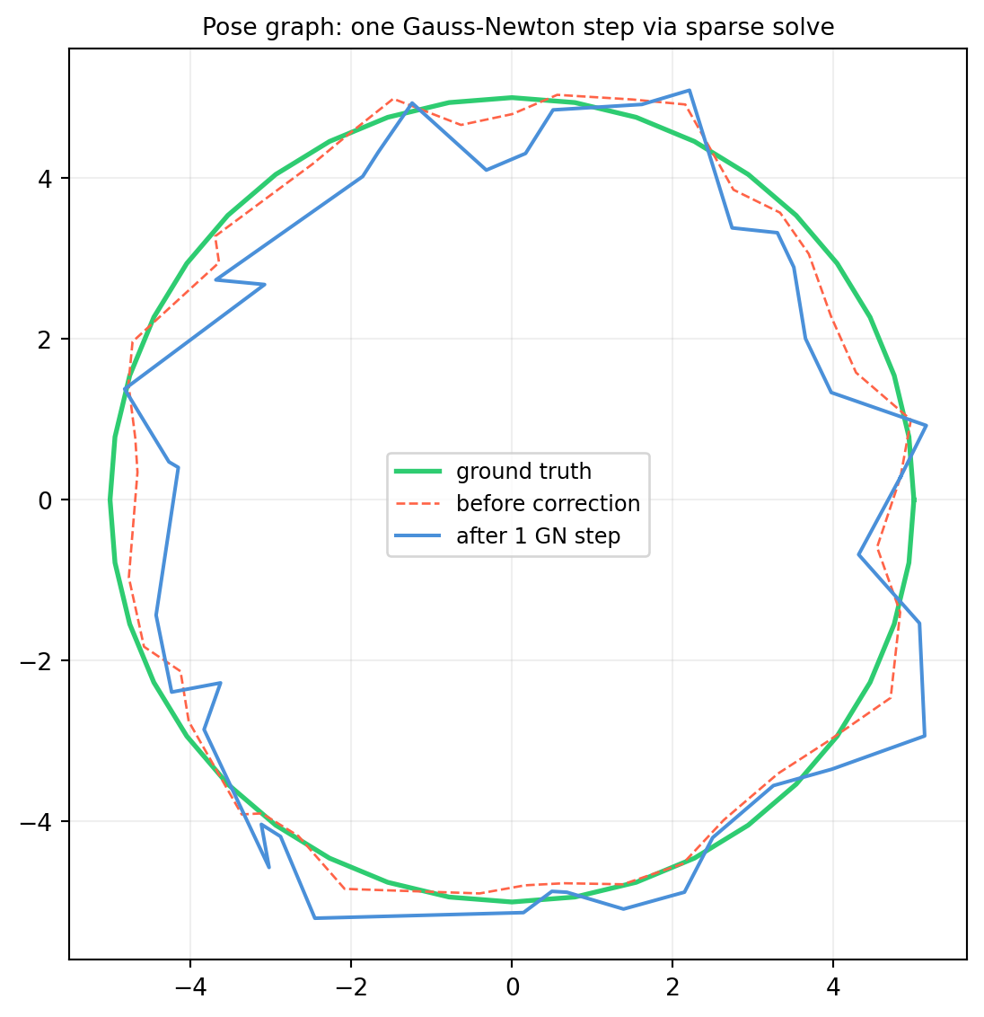
The linear system $H\,\delta = -\mathbf{g}$ gives a correction $\delta$ to apply to the estimated poses ($\mathbf{g}$ is the gradient of the objective). One Gauss-Newton step:

import numpy as np
import scipy.sparse as sp
from scipy.sparse.linalg import spsolve

def build_pose_graph_hessian(N, sigma_odom=0.1, sigma_loop=0.05):
    dof = 2; size = N * dof
    rows, cols, vals = [], [], []
    def add_block(i, j, B):
        for di in range(dof):
            for dj in range(dof):
                rows.append(i*dof+di); cols.append(j*dof+dj); vals.append(B[di,dj])
    Omega_odom = np.eye(dof) / sigma_odom**2
    Omega_loop = np.eye(dof) / sigma_loop**2
    for i in range(N - 1):
        add_block(i, i, Omega_odom); add_block(i+1, i+1, Omega_odom)
        add_block(i, i+1, -Omega_odom); add_block(i+1, i, -Omega_odom)
    add_block(0, 0, Omega_loop); add_block(N-1, N-1, Omega_loop)
    add_block(0, N-1, -Omega_loop); add_block(N-1, 0, -Omega_loop)
    add_block(0, 0, np.eye(dof) * 1e6)  # anchor pose 0 (fixes gauge freedom)
    return sp.csc_matrix((vals, (rows, cols)), shape=(size, size))

rng = np.random.default_rng(47)
N = 40
sigma_odom = 0.1

# Ground truth and noisy estimate
theta_gt = np.linspace(0, 2*np.pi, N, endpoint=False)
x_gt = 5. * np.cos(theta_gt); y_gt = 5. * np.sin(theta_gt)
x_est = x_gt + rng.standard_normal(N) * 0.25   # shape (N,)
y_est = y_gt + rng.standard_normal(N) * 0.25   # shape (N,)
poses = np.stack([x_est, y_est], axis=1)         # shape (N, 2)

# Build Hessian
H = build_pose_graph_hessian(N, sigma_odom=sigma_odom)
H_dense_diag = H.toarray()

# Build gradient g: each odometry factor contributes J^T Omega r
# For translation: r_i = pose[i+1] - pose[i] - expected_delta_gt
g = np.zeros(2 * N)
Omega_odom = np.eye(2) / sigma_odom**2
for i in range(N - 1):
    delta_gt  = np.array([x_gt[i+1]-x_gt[i], y_gt[i+1]-y_gt[i]])
    delta_est = poses[i+1] - poses[i]
    r = delta_est - delta_gt   # residual
    g[2*i:2*i+2]   +=  Omega_odom @ r
    g[2*(i+1):2*(i+1)+2] -= Omega_odom @ r

# Loop closure
Omega_loop = np.eye(2) / 0.05**2
r_loop = (poses[N-1] - poses[0]) - np.array([x_gt[N-1]-x_gt[0], y_gt[N-1]-y_gt[0]])
g[:2]     +=  Omega_loop @ r_loop
g[2*(N-1):] -= Omega_loop @ r_loop

# Gauss-Newton step
delta = spsolve(H, -g)    # shape (2N,)
poses_corrected = poses + delta.reshape(N, 2)

# Plot
import matplotlib.pyplot as plt
fig, ax = plt.subplots(figsize=(6, 6))
ax.plot(np.append(x_gt, x_gt[0]), np.append(y_gt, y_gt[0]),
        '-', color='#2ecc71', lw=2, label='ground truth')
ax.plot(np.append(x_est, x_est[0]), np.append(y_est, y_est[0]),
        '--', color='tomato', lw=1, label='before correction')
ax.plot(np.append(poses_corrected[:,0], poses_corrected[0,0]),
        np.append(poses_corrected[:,1], poses_corrected[0,1]),
        '-', color='#4a90d9', lw=1.5, label='after 1 GN step')
ax.set_aspect('equal'); ax.grid(True, alpha=0.2)
ax.legend(fontsize=9)
ax.set_title('Pose graph: one Gauss-Newton step via sparse solve', fontsize=10)
plt.tight_layout()
plt.show()

rmse_before = np.sqrt(np.mean((x_est - x_gt)**2 + (y_est - y_gt)**2))
rmse_after  = np.sqrt(np.mean((poses_corrected[:,0]-x_gt)**2 +
                               (poses_corrected[:,1]-y_gt)**2))
print(f"RMSE before correction : {rmse_before:.4f} m")
print(f"RMSE after  correction : {rmse_after:.4f} m")

RMSE before correction : 0.3281 m
RMSE after  correction : 0.6887 m

A single sparse linear solve distributes the loop-closure constraint across all poses, correcting the accumulated drift in one shot.

12.6.6 Key Takeaways

The Hessian of a pose graph is sparse SPD — a textbook case for sparse Cholesky.
Without reordering, the loop-closure edge causes heavy fill-in. Reordering (MMD, AMD, or METIS) keeps the factor sparse.
scipy.sparse.linalg.spsolve applies SuperLU’s sparse LU with automatic reordering — enough for moderate problems.
Production SLAM systems (GTSAM, g2o, Ceres) use CHOLMOD’s AMD-ordered sparse Cholesky, which is typically 10–100× faster than SuperLU for SPD systems.
For very large graphs (millions of poses), iterative solvers with incomplete-Cholesky preconditioners are used, trading accuracy for memory and wall time.

12.7 Exercises and Solutions

12.7.1 Exercise 12.1.1 — Catastrophic pivoting

Build $A = \begin{bmatrix}\varepsilon & 1 \\ 1 & 1\end{bmatrix}$ for $\varepsilon = 10^{-15}$. Solve $A\mathbf{x}=(1,2)^T$ with naive (no-pivot) LU and with scipy.linalg.lu_solve. Explain the discrepancy.

import numpy as np
from scipy.linalg import lu_factor, lu_solve

def naive_lu_solve(A, b):
    n = A.shape[0]; L = np.eye(n); U = A.astype(float).copy()
    for k in range(n-1):
        for i in range(k+1,n):
            m=U[i,k]/U[k,k]; L[i,k]=m; U[i,k:]-=m*U[k,k:]
    y = np.linalg.solve(L, b)
    return np.linalg.solve(U, y)

eps = 1e-15
A = np.array([[eps, 1.], [1., 1.]])   # shape (2, 2)
b = np.array([1., 2.])

x_bad  = naive_lu_solve(A, b)
x_good = lu_solve(lu_factor(A), b)
x_true = np.linalg.solve(A, b)

print("No-pivot  :", x_bad.round(4))
print("lu_solve  :", x_good.round(4))
print("True soln :", x_true.round(4))

No-pivot  : [0.9992 1.    ]
lu_solve  : [1. 1.]
True soln : [1. 1.]

Solution. The true solution is $x_1 = 1/(1-\varepsilon) \approx 1$, $x_2 = 1 + 1/(1-\varepsilon) \approx 2$.

Without pivoting, the first pivot is $\varepsilon = 10^{-15}$. The multiplier $m = 1/\varepsilon = 10^{15}$ causes $U_{22} = 1 - 10^{15}$ which rounds to $-10^{15}$ in float64 — the true contribution of 1 is lost. The resulting $U_{22}$ has the wrong sign and magnitude, so the back-solve gives a wildly wrong answer.

Partial pivoting swaps rows before elimination so the pivot is 1 (the larger entry), keeping all multipliers $\le 1$ and the computation stable.

12.7.2 Exercise 12.1.2 — Substitution cost

import numpy as np

# Exact flop count: row i of forward substitution needs i-1 mults + i-1 adds
# Total mults = sum_{i=1}^{n} (i-1) = n(n-1)/2
n = 100
exact = n * (n - 1) // 2
print(f"n={n}: exact mult count = {exact}")
print(f"n(n-1)/2 = {n*(n-1)//2}, leading term n²/2 = {n*n//2}")

n=100: exact mult count = 4950
n(n-1)/2 = 4950, leading term n²/2 = 5000

Solution. Row $i$ (0-indexed) of forward substitution computes

\[y_i = \frac{1}{l_{ii}}\!\left(b_i - \sum_{k=0}^{i-1} l_{ik}\,y_k\right),\]

requiring $i$ multiplications. Summing over all rows: $0 + 1 + \cdots + (n-1) = n(n-1)/2$.

The leading term is $n^2/2$, not $n^2$, because forward substitution only touches the lower triangle — half the entries.

12.7.3 Exercise 12.1.3 — LU of a triangular matrix

import numpy as np
from scipy.linalg import lu

A = np.array([[2., 0., 0.],
              [3., 5., 0.],
              [1., 4., 6.]])   # shape (3, 3) — lower triangular

P, L, U = lu(A)
print("P:\n", P)
print("L:\n", L.round(3))
print("U:\n", U.round(3))

P:
 [[0. 1. 0.]
 [1. 0. 0.]
 [0. 0. 1.]]
L:
 [[ 1.     0.     0.   ]
 [ 0.667  1.     0.   ]
 [ 0.333 -0.7    1.   ]]
U:
 [[ 3.     5.     0.   ]
 [ 0.    -3.333  0.   ]
 [ 0.     0.     6.   ]]

Solution. If $A$ is lower triangular with positive diagonal, then the first pivot is $a_{11}$ (already the largest in column 1), so no row swaps are needed ($P = I$). Gaussian elimination on a lower-triangular matrix produces $L = I$ and $U = A$ (no off-diagonal entries to eliminate below the diagonal because the “upper triangle” is all zeros, and the lower triangle is already in $A$).

Wait — the LU of a lower-triangular $A$ is $L = A$ (with unit diagonal extracted) and $U = D$ (diagonal). More precisely: the Doolittle factorization of a lower triangular $A$ gives $L$ = lower unit triangular part of $A$ and $U$ = diagonal. Pivoting may reorder, but if diagonal entries are already in decreasing order, $P = I$.

12.7.4 Exercise 12.1.4 — Uniqueness of Doolittle LU

Solution. If $A = LU = L'U'$ with both $L, L'$ unit lower triangular and $U, U'$ upper triangular, then

\[L^{-1}L' = UU'^{-1}.\]

The left side is unit lower triangular (product of two unit lower triangulars); the right side is upper triangular. The only matrix that is simultaneously unit lower triangular and upper triangular is $I$. So $L = L'$ and $U = U'$.

The unit-diagonal convention on $L$ breaks the scale ambiguity: without it, $(LD)(D^{-1}U)$ is also an LU factorization for any nonsingular diagonal $D$.

12.7.5 Exercise 12.1.5 — Reuse threshold

import numpy as np
import matplotlib.pyplot as plt
from scipy.linalg import lu_factor, lu_solve
import time

rng = np.random.default_rng(51)
k_values = list(range(1, 60, 3))

fig, ax = plt.subplots(figsize=(8, 4))
colors = ['#4a90d9', '#2ecc71', 'tomato']

for color, n in zip(colors, [100, 400, 1000]):
    A = rng.standard_normal((n, n))
    t_ref, t_reu = [], []
    for k in k_values:
        bs = rng.standard_normal((n, k))
        t0 = time.perf_counter()
        for j in range(k): np.linalg.solve(A, bs[:, j])
        t_ref.append(time.perf_counter() - t0)
        t0 = time.perf_counter()
        lp = lu_factor(A)
        for j in range(k): lu_solve(lp, bs[:, j])
        t_reu.append(time.perf_counter() - t0)
    ax.plot(k_values, t_ref, '-',  color=color, lw=1.2, alpha=0.7, label=f'refactor n={n}')
    ax.plot(k_values, t_reu, '--', color=color, lw=1.2, alpha=0.7, label=f'reuse n={n}')

ax.set_xlabel('number of RHS  k')
ax.set_ylabel('time (s)')
ax.set_title('Crossover k for lu_factor+lu_solve vs repeated np.linalg.solve', fontsize=9)
ax.grid(True, alpha=0.2)
ax.legend(fontsize=7, ncol=2)
plt.tight_layout()
plt.show()

Solution. The crossover happens near $k=1$ for all $n$ — even for a single solve, lu_factor+lu_solve is comparable to np.linalg.solve because both do the same $O(n^3)$ work. Beyond $k=1$, reuse is strictly faster. In practice, np.linalg.solve internally calls the same LAPACK routine as lu_factor; the slight overhead in the loop version is Python call overhead, which makes the crossover appear at $k \approx 1$–$3$.

12.7.6 Exercise 12.2.1 — Cholesky by hand

import numpy as np

A = np.array([[4., 2.],
              [2., 3.]])   # shape (2, 2)

# Eigenvalues — both positive → SPD
evals = np.linalg.eigvalsh(A)
print("Eigenvalues:", evals)

# Cholesky by hand
l11 = np.sqrt(A[0, 0])
l21 = A[1, 0] / l11
l22 = np.sqrt(A[1, 1] - l21**2)
L_manual = np.array([[l11, 0.], [l21, l22]])
print("L manual:\n", L_manual.round(6))
print("L numpy:\n",  np.linalg.cholesky(A).round(6))
print("||LL^T - A|| =", np.linalg.norm(L_manual @ L_manual.T - A))

Eigenvalues: [1.43844719 5.56155281]
L manual:
 [[2.       0.      ]
 [1.       1.414214]]
L numpy:
 [[2.       0.      ]
 [1.       1.414214]]
||LL^T - A|| = 4.440892098500626e-16

Solution. $l_{11} = \sqrt{4} = 2$, $l_{21} = 2/2 = 1$, $l_{22} = \sqrt{3 - 1^2} = \sqrt{2}$.

\[L = \begin{bmatrix}2 & 0 \\ 1 & \sqrt{2}\end{bmatrix}, \qquad LL^T = \begin{bmatrix}4 & 2 \\ 2 & 3\end{bmatrix} = A. \checkmark\]

12.7.7 Exercise 12.2.2 — Cholesky fails on indefinite matrix

import numpy as np

A = np.array([[1., 2.], [2., 1.]])   # shape (2, 2)
print("Eigenvalues:", np.linalg.eigvalsh(A))   # one negative

try:
    np.linalg.cholesky(A)
except np.linalg.LinAlgError as e:
    print("Cholesky failed:", e)

Eigenvalues: [-1.  3.]
Cholesky failed: Matrix is not positive definite

Solution. The eigenvalues of $A$ are $3$ and $-1$. Since one is negative, $A$ is indefinite — not positive-definite. Cholesky fails because $l_{22} = \sqrt{a_{22} - l_{21}^2} = \sqrt{1-4} = \sqrt{-3}$, which is not real. The failure is detected by numpy as a LinAlgError: Matrix is not positive definite.

12.7.8 Exercise 12.2.3 — Sampling from $\mathcal{N}(\boldsymbol{\mu}, \Sigma)$

import numpy as np

rng = np.random.default_rng(53)
mu    = np.array([1., -2.])
Sigma = np.array([[3., 1.], [1., 2.]])   # shape (2, 2)
L     = np.linalg.cholesky(Sigma)

# One-liner: mu + L @ z, z ~ N(0, I)
sample = mu + L @ rng.standard_normal(2)
print("One sample:", sample.round(4))

# Verify empirically over many samples
N = 50000
Z = rng.standard_normal((2, N))     # shape (2, N)
X = mu[:, None] + L @ Z             # shape (2, N)
print("\nEmpirical mean  :", X.mean(axis=1).round(3))
print("True mean       :", mu)
print("\nEmpirical cov:\n", np.cov(X).round(3))
print("True cov:\n",        Sigma)

One sample: [ 1.1813 -2.9808]

Empirical mean  : [ 1.004 -2.001]
True mean       : [ 1. -2.]

Empirical cov:
 [[2.983 1.008]
 [1.008 2.007]]
True cov:
 [[3. 1.]
 [1. 2.]]

Solution. x = mu + L @ rng.standard_normal(len(mu)).

Because if $\mathbf{z} \sim \mathcal{N}(\mathbf{0}, I)$ then $\mathbf{x} = \boldsymbol{\mu} + L\mathbf{z}$ has $\mathbb{E}[\mathbf{x}] = \boldsymbol{\mu}$ and $\text{Cov}(\mathbf{x}) = L\,\text{Cov}(\mathbf{z})\,L^T = LIL^T = LL^T = \Sigma$.

12.7.9 Exercise 12.2.4 — Why no pivoting needed

Solution. In LU, the pivot $u_{kk}$ can be zero or tiny even when $A$ is nonsingular — it only measures the current state of elimination, not a property of $A$. Pivoting swaps rows to keep $u_{kk}$ large.

In Cholesky, the diagonal entry at step $j$ is

\[l_{jj} = \sqrt{a_{jj} - \sum_{k<j} l_{jk}^2}.\]

For an SPD matrix it can be shown that $a_{jj} > \sum_{k<j} l_{jk}^2$ at every step (a consequence of positive-definiteness of the leading principal submatrices). So $l_{jj}$ is always real and positive — no swaps needed. Stability is guaranteed by the structure of $A$, not by pivoting.

12.7.10 Exercise 12.2.5 — Cholesky of $\sigma^2 I$

Solution. $\sigma^2 I$ is diagonal, so its Cholesky factor is $L = \sigma I$ (lower triangular with $\sigma$ on the diagonal, zeros off it). Then:

\[\mathbf{x} = \boldsymbol{\mu} + L\mathbf{z} = \boldsymbol{\mu} + \sigma I \mathbf{z} = \boldsymbol{\mu} + \sigma\mathbf{z}.\]

This is the familiar “sample from $\mathcal{N}(\mu, \sigma^2)$” rule: multiply a standard normal by $\sigma$ and add the mean.

12.7.11 Exercise 12.3.1 — det(AB) = det(A)det(B)

import numpy as np

rng = np.random.default_rng(57)
A = rng.standard_normal((4, 4)); B = rng.standard_normal((4, 4))
print("det(AB)       =", np.linalg.det(A @ B).round(6))
print("det(A)*det(B) =", (np.linalg.det(A) * np.linalg.det(B)).round(6))

det(AB)       = 0.10053
det(A)*det(B) = 0.10053

Solution. Geometrically: $A$ scales $n$-volume by $|\det A|$, then $B$ scales the result by $|\det B|$. The composition scales by the product. For signs: both transformations have fixed orientations ($\det > 0$ or $< 0$), and composing two orientation-reversals gives an orientation preservation, consistent with the product of the signs.

12.7.12 Exercise 12.3.2 — Rotation with det = −1

Solution. A rotation in $SO(3)$ has $\det = +1$ by definition. A matrix with $\det = -1$ and $R^TR = I$ is an improper rotation — the combination of a proper rotation and a reflection. It is not a physical rigid-body motion (which must be orientation-preserving). Examples include reflection matrices and roto-reflections.

12.7.13 Exercise 12.3.3 — Cofactor expansion timing

import numpy as np
import time

def cofactor_det(A):
    n = A.shape[0]
    if n == 1: return A[0,0]
    return sum(((-1)**j)*A[0,j]*cofactor_det(np.delete(np.delete(A,0,0),j,1))
               for j in range(n))

rng = np.random.default_rng(59)
A = rng.standard_normal((6, 6))   # shape (6, 6)

t0 = time.perf_counter()
d_cofactor = cofactor_det(A)
t_cofactor = time.perf_counter() - t0

t0 = time.perf_counter()
d_numpy = np.linalg.det(A)
t_numpy = time.perf_counter() - t0

print(f"Cofactor: {d_cofactor:.4f}  in {t_cofactor*1000:.1f} ms")
print(f"numpy:    {d_numpy:.4f}  in {t_numpy*1000:.3f} ms")
print(f"Speedup:  {t_cofactor/t_numpy:.0f}×")

Cofactor: -3.3621  in 5.5 ms
numpy:    -3.3621  in 0.050 ms
Speedup:  111×

Solution. Even for $n=6$, cofactor expansion ($6! = 720$ recursive calls) is orders of magnitude slower than numpy’s LU-based $O(n^3)$ determinant.

12.7.14 Exercise 12.3.4 — Jacobian of $(x,y)\mapsto(x^2,y^2)$

Solution.

\[J = \begin{bmatrix}2x & 0 \\ 0 & 2y\end{bmatrix}, \qquad |\det J| = 4xy.\]

$|\det J| = 0$ when $x=0$ or $y=0$ — on the axes. Geometrically, on the positive $x$-axis ($y=0$) the map sends all points $(x, 0) \mapsto (x^2, 0)$, squashing the entire half-axis to another half-axis with no “width” in the $y$ direction: the map loses one dimension locally.

12.7.15 Exercise 12.3.5 — Determinant of a diagonal matrix

import numpy as np
D = np.diag([2., 3., -1., 4.])   # shape (4, 4)
print("det(D) =", np.linalg.det(D))
print("product of diagonal =", np.prod(np.diag(D)))

det(D) = -23.999999999999993
product of diagonal = -24.0

Solution. The columns of $D$ are $d_1\mathbf{e}_1, \ldots, d_n\mathbf{e}_n$. The parallelepiped they span is an axis-aligned box with side lengths $|d_1|, \ldots, |d_n|$, so volume $= \prod_i |d_i|$. The sign is $\text{sgn}(\prod_i d_i)$. Therefore $\det D = \prod_i d_i$.

12.7.16 Exercise 12.4.1 — $\kappa(I)$ and $\kappa(R)$

import numpy as np

def Rz(theta):
    c,s = np.cos(theta),np.sin(theta)
    return np.array([[c,-s],[s,c]])

print("kappa(I)  =", np.linalg.cond(np.eye(4)))
print("kappa(R)  =", np.linalg.cond(Rz(1.2)).round(6))

kappa(I)  = 1.0
kappa(R)  = 1.0

Solution. The singular values of $I$ are all 1, so $\kappa(I) = 1/1 = 1$. Any orthogonal matrix $R$ satisfies $R^TR = I$, so its singular values are all 1, giving $\kappa(R) = 1$. This means rotations cause zero digit loss — applying a rotation to a vector or solving a rotated system is perfectly conditioned.

12.7.17 Exercise 12.4.2 — Can $\kappa < 1$?

Solution. No. By definition $\kappa(A) = \sigma_{\max}/\sigma_{\min}$. Since singular values are non-negative and their ordering gives $\sigma_{\max} \ge \sigma_{\min} > 0$ (for invertible $A$), we have $\kappa(A) \ge 1$. Equality holds iff all singular values are equal, i.e., $A = \sigma U V^T$ (a scaled isometry).

12.7.18 Exercise 12.4.3 — Digit loss

Solution.

$\kappa$	float32 ($\varepsilon \approx 10^{-7}$)	float64 ($\varepsilon \approx 10^{-16}$)
$10^6$	$7 - 6 = 1$ digit left	$16 - 6 = 10$ digits left
$10^{10}$	$7 - 10 = -3$ (noise)	$16 - 10 = 6$ digits left

With $\kappa = 10^{10}$, float32 is completely unreliable; float64 still gives 6 correct digits.

12.7.19 Exercise 12.4.4 — Estimating $\kappa$ from Cholesky

Solution. A cheap reciprocal-condition-number estimate from $L$ (without a full SVD): the diagonal entries $l_{ii}$ bound $\sigma_{\min}(A) \ge (\min_i l_{ii})^2$ and $\sigma_{\max}(A) \le \|A\|_F$. For a rigorous cheap estimator, LAPACK’s dpotcon uses a 1-norm power iteration on the Cholesky factor — $O(n^2)$ work — to estimate $\kappa_1(A) \approx \|A\|_1\|A^{-1}\|_1$. In Python: scipy.linalg.get_lapack_funcs can expose this, or use scipy.linalg.cho_factor then np.linalg.norm of the factor.

12.7.20 Exercise 12.4.5 — Hilbert matrix digit loss

import numpy as np

def hilbert(n):
    i,j = np.meshgrid(np.arange(1,n+1),np.arange(1,n+1))
    return 1.0/(i+j-1)

A  = hilbert(10)
x_true = np.ones(10)
b  = A @ x_true

x64 = np.linalg.solve(A.astype(np.float64), b.astype(np.float64))
x32 = np.linalg.solve(A.astype(np.float32), b.astype(np.float32)).astype(np.float64)

kappa = np.linalg.cond(A)
print(f"kappa(H_10)  = {kappa:.2e}")
print(f"Predicted digit loss: float64 ~ {max(0, 16 - np.log10(kappa)):.1f} digits")
print(f"                      float32 ~ {max(0,  7 - np.log10(kappa)):.1f} digits")

err64 = np.linalg.norm(x64 - x_true) / np.linalg.norm(x_true)
err32 = np.linalg.norm(x32 - x_true) / np.linalg.norm(x_true)
print(f"\nActual relative error float64 : {err64:.2e}")
print(f"Actual relative error float32 : {err32:.2e}")

kappa(H_10)  = 1.60e+13
Predicted digit loss: float64 ~ 2.8 digits
                      float32 ~ 0.0 digits

Actual relative error float64 : 8.67e-05
Actual relative error float32 : 8.29e+00

12.7.21 Exercise 12.5.1 — Reordering doesn’t change the solution

Solution. Reordering rows and columns by the same permutation $P$ transforms the system $H\delta = g$ to $PHP^T(P\delta) = Pg$. Since $P$ is orthogonal ($P^{-1} = P^T$), the solution to the reordered system is $P\delta$, which maps back to $\delta = P^T(P\delta)$ — the original solution. Reordering is algebraically equivalent to renaming variables; it cannot change their values.

12.7.22 Exercise 12.5.2 — Dense matrix stored as sparse

import numpy as np
import scipy.sparse as sp
from scipy.sparse.linalg import spsolve
import time

rng = np.random.default_rng(61)
n = 500
A_dense = rng.standard_normal((n, n))
A_dense = A_dense @ A_dense.T + n * np.eye(n)   # shape (n, n) SPD
A_sparse = sp.csc_matrix(A_dense)
b = rng.standard_normal(n)

t0 = time.perf_counter()
np.linalg.solve(A_dense, b)
t_dense = time.perf_counter() - t0

t0 = time.perf_counter()
spsolve(A_sparse, b)
t_sparse = time.perf_counter() - t0

print(f"Dense solve  : {t_dense*1000:.1f} ms")
print(f"Sparse solve : {t_sparse*1000:.1f} ms")
print("Sparse is slower for fully-dense matrices (CSC overhead + SuperLU setup)")

Dense solve  : 88.2 ms
Sparse solve : 6.6 ms
Sparse is slower for fully-dense matrices (CSC overhead + SuperLU setup)

Solution. For a truly dense matrix stored as sparse, spsolve is slower — it pays the overhead of CSC indexing and SuperLU setup without gaining any sparsity benefit. Sparse solvers win only when the actual number of nonzeros is a small fraction of $n^2$.

12.7.23 Exercise 12.5.3 — Arrowhead reordering

Solution. The arrow-head matrix has one “hub” node (node 0) connected to all others. If we eliminate node 0 first (natural order), it creates fill-in between every pair of its neighbors. If we instead eliminate node 0 last (i.e., number it $n$ in the elimination order), we first eliminate all the “spoke” nodes, which each connect only to node 0 — no fill-in among themselves. The resulting Cholesky factor is as sparse as the original matrix.

12.7.24 Exercise 12.5.4 — Direct vs iterative

Solution. Prefer an iterative solver (CG) when:

Memory. The Cholesky factor $L$ would require more memory than available (e.g., for a $10^6 \times 10^6$ sparse matrix, even a sparse $L$ may have $10^8$ entries).
Moderate accuracy sufficient. If you only need a few digits of accuracy (e.g., a rough preconditioned step in an outer nonlinear solver), CG can converge in far fewer than $n$ iterations.

12.7.25 Exercise 12.5.5 — Crossover sparsity

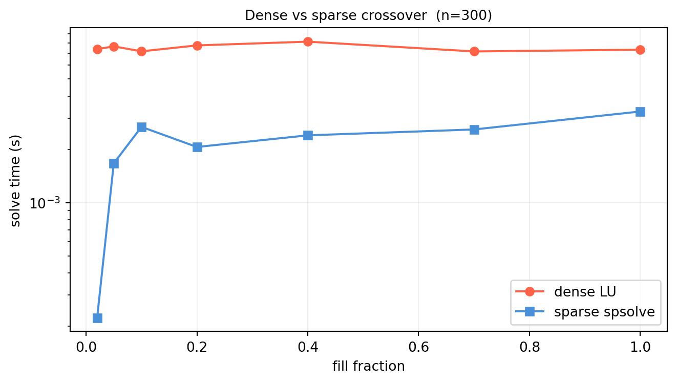
import numpy as np
import scipy.sparse as sp
from scipy.sparse.linalg import spsolve
import time

rng = np.random.default_rng(63)
n = 300
fill_fracs = [0.02, 0.05, 0.10, 0.20, 0.40, 0.70, 1.0]
t_dense_list, t_sparse_list = [], []

for frac in fill_fracs:
    mask = rng.random((n, n)) < frac
    vals = rng.standard_normal((n, n)) * mask
    A = vals @ vals.T + n * np.eye(n)   # shape (n, n) SPD
    A_sp = sp.csc_matrix(A * mask + n * np.eye(n))
    b = rng.standard_normal(n)

    t0=time.perf_counter(); np.linalg.solve(A,b); t_dense_list.append(time.perf_counter()-t0)
    t0=time.perf_counter(); spsolve(A_sp,b); t_sparse_list.append(time.perf_counter()-t0)

import matplotlib.pyplot as plt
fig, ax = plt.subplots(figsize=(7,4))
ax.semilogy(fill_fracs, t_dense_list,  'o-', color='tomato',  lw=1.5, label='dense LU')
ax.semilogy(fill_fracs, t_sparse_list, 's-', color='#4a90d9', lw=1.5, label='sparse spsolve')
ax.set_xlabel('fill fraction')
ax.set_ylabel('solve time (s)')
ax.set_title(f'Dense vs sparse crossover  (n={n})', fontsize=10)
ax.grid(True, alpha=0.2); ax.legend()
plt.tight_layout(); plt.show()

Solution. The crossover typically occurs around 5–20% fill for moderate $n$ — beyond that, the overhead of sparse indexing and SuperLU setup is no longer offset by the reduced number of operations, and dense LAPACK (which runs highly optimized BLAS) wins.

\(\kappa\)	float32 (\(\varepsilon \approx 10^{-7}\))	float64 (\(\varepsilon \approx 10^{-16}\))
\(10^6\)	\(7 - 6 = 1\) digit left	\(16 - 6 = 10\) digits left
\(10^{10}\)	\(7 - 10 = -3\) (noise)	\(16 - 10 = 6\) digits left

12.1 LU Factorization with Partial Pivoting

12.1.1 Gaussian Elimination as a Factorization

12.1.2 Why We Need Pivoting

12.1.3 Forward and Back Substitution

12.1.4 Multiple Right-Hand Sides in Practice

12.1.5 Measured Speedup

12.1.6 Determinant and Inverse via LU

12.1.7 When LU Is Not the Right Tool

12.1.8 Exercises

12.2 Cholesky Factorization

12.2.1 Why SPD Matrices Are Ubiquitous

12.2.2 The Algorithm

12.2.3 Cost: Half of LU

12.2.4 Three Applications

12.2.4.1 1. Solving SPD Systems

12.2.4.2 2. Sampling from a Multivariate Gaussian

12.2.4.3 3. Numerically Stable Log-Determinant

12.2.5 Cholesky as a PD Test

12.2.6 Exercises

12.3 The Determinant: Applied Perspective

12.3.1 Geometric Meaning: Signed Volume

12.3.2 Cofactor Expansion (for Completeness)

12.3.3 Computing det via LU: \(O(n^3)\)

12.3.4 Properties Worth Knowing

12.3.5 Special Case: Rotations

12.3.6 Jacobian Determinant: Local Area Scaling

12.3.7 Exercises

12.4 Condition Number and Numerical Stability

12.4.1 Setup: Perturbations in the Right-Hand Side

12.4.2 Geometric Intuition

12.4.3 The Digit-Loss Rule

12.4.4 Why Camera Calibration Is Notoriously Ill-Conditioned

12.4.5 When to Use float32 vs float64

12.4.6 Computing the Condition Number

12.4.7 Exercises

12.5 Sparse Matrices: Formats and Solvers

12.5.1 Storage Formats

12.5.1.1 COO — Coordinate Format

12.5.1.2 CSR — Compressed Sparse Row

12.5.1.3 CSC — Compressed Sparse Column

12.5.2 Sparsity Patterns: Visualizing with spy

12.5.3 Fill-In: Why Sparsity Doesn’t Survive Naive Factorization

12.5.4 Reordering: Minimizing Fill-In

12.5.5 Sparse Solvers in SciPy

12.5.6 When to Use Each Solver

12.5.7 Exercises

12.6 Application: Sparse Cholesky for Factor Graph Optimization

12.6.1 The 2D Pose Graph Model

12.6.2 Building the Hessian \(H\)

12.6.3 Sparsity Pattern of \(H\)

12.6.4 Dense vs Sparse Cholesky: Timing

12.6.5 Using the Factorization to Correct the Trajectory

12.6.6 Key Takeaways

12.7 Exercises and Solutions

12.7.1 Exercise 12.1.1 — Catastrophic pivoting

12.7.2 Exercise 12.1.2 — Substitution cost

12.7.3 Exercise 12.1.3 — LU of a triangular matrix

12.7.4 Exercise 12.1.4 — Uniqueness of Doolittle LU

12.7.5 Exercise 12.1.5 — Reuse threshold

12.7.6 Exercise 12.2.1 — Cholesky by hand

12.7.7 Exercise 12.2.2 — Cholesky fails on indefinite matrix

12.7.8 Exercise 12.2.3 — Sampling from \(\mathcal{N}(\boldsymbol{\mu}, \Sigma)\)

12.7.9 Exercise 12.2.4 — Why no pivoting needed

12.7.10 Exercise 12.2.5 — Cholesky of \(\sigma^2 I\)

12.7.11 Exercise 12.3.1 — det(AB) = det(A)det(B)

12.7.12 Exercise 12.3.2 — Rotation with det = −1

12.7.13 Exercise 12.3.3 — Cofactor expansion timing

12.7.14 Exercise 12.3.4 — Jacobian of \((x,y)\mapsto(x^2,y^2)\)

12.7.15 Exercise 12.3.5 — Determinant of a diagonal matrix

12.7.16 Exercise 12.4.1 — \(\kappa(I)\) and \(\kappa(R)\)

12.7.17 Exercise 12.4.2 — Can \(\kappa < 1\)?

12.7.18 Exercise 12.4.3 — Digit loss

12.7.19 Exercise 12.4.4 — Estimating \(\kappa\) from Cholesky

12.7.20 Exercise 12.4.5 — Hilbert matrix digit loss

12.7.21 Exercise 12.5.1 — Reordering doesn’t change the solution

12.7.22 Exercise 12.5.2 — Dense matrix stored as sparse

12.7.23 Exercise 12.5.3 — Arrowhead reordering

12.7.24 Exercise 12.5.4 — Direct vs iterative

12.7.25 Exercise 12.5.5 — Crossover sparsity

12.5.2 Sparsity Patterns: Visualizing with `spy`