24  Lie Groups and Lie Algebras

24.1 Motivation

In Chapter 8 you learned that every 3D rotation can be stored as a matrix \(R \in \text{SO}(3)\), and in Chapter 9 you chained rotations and translations into rigid-body transforms \(T \in \text{SE}(3)\). Applying a stored transform is easy: a single matrix multiply. Doing calculus on transforms is harder, and three standard operations break badly when you treat rotations as ordinary matrices or angle tuples.

Averaging. Given measured orientations \(R_1, \ldots, R_n \in \text{SO}(3)\), the arithmetic mean \(\bar{R} = \frac{1}{n}\sum_i R_i\) is generally not a rotation matrix: \(\det(\bar{R}) \neq 1\) and \(\bar{R}^T \bar{R} \neq I\). The naive mean drifts further off the manifold as the rotations spread further apart.

Smooth interpolation. Lerping the nine matrix entries between \(R_1\) and \(R_2\) produces non-orthogonal intermediate frames. Lerping Euler angles (\(\alpha, \beta, \gamma\)) takes an incorrect path through orientation space and suffers from gimbal lock: when the middle angle \(\beta\) reaches \(\pm 90°\), the first and third axes align and the parametrization loses a degree of freedom, causing sudden large jumps in the angle values.

Gradient-based optimization. In bundle adjustment, pose-graph SLAM, and calibration, the unknowns are rotation matrices. A gradient step \(R \leftarrow R - \alpha\,\nabla f\) immediately leaves \(\text{SO}(3)\). Projecting back (e.g., via SVD) after each step breaks the gradient flow and is expensive.

The fix for all three is to recognize that \(\text{SO}(3)\) is a smooth manifold: near any point it looks locally like \(\mathbb{R}^3\). The tangent space at the identity \(I\) is a linear space called the Lie algebra \(\mathfrak{so}(3)\). The exponential map \(\exp: \mathfrak{so}(3) \to \text{SO}(3)\) connects the flat algebra to the curved group, enabling a single clean pattern:

\[ \underbrace{\text{compute in } \mathfrak{so}(3)}_{\text{ordinary linear algebra}} \;\;\xrightarrow{\;\exp\;}\;\; \underbrace{\text{return to SO}(3)}_{\text{valid rotation}} \]

This chapter builds that machinery for \(\text{SO}(3)\) (§§24.2–24.4) and \(\text{SE}(3)\) (§24.5), then shows how it powers optimization on curved spaces (§24.6).

---

24.1.1 Naive Averaging Leaves the Group

The plot below sweeps the angular separation between two rotations from \(0°\) to \(180°\) and records how far the arithmetic mean drifts from \(\text{SO}(3)\).

import numpy as np
import matplotlib.pyplot as plt
from scipy.spatial.transform import Rotation

rng = np.random.default_rng(42)
n_pts = 120
thetas = np.linspace(0.0, np.pi, n_pts)    # shape (120,)

det_err   = np.zeros(n_pts)                 # shape (120,)
ortho_err = np.zeros(n_pts)                 # shape (120,)

axis = np.array([1.0, 1.0, 0.0]) / np.sqrt(2.0)    # fixed axis

for i, th in enumerate(thetas):
    R_a = np.eye(3)                                           # shape (3, 3)
    R_b = Rotation.from_rotvec(th * axis).as_matrix()        # shape (3, 3)
    Mm  = (R_a + R_b) / 2.0                                  # shape (3, 3)
    det_err[i]   = abs(np.linalg.det(Mm) - 1.0)
    ortho_err[i] = np.linalg.norm(Mm.T @ Mm - np.eye(3))

fig, axes = plt.subplots(1, 2, figsize=(11, 4))

ax = axes[0]
ax.plot(np.degrees(thetas), det_err, color='#4a90d9', lw=2)
ax.set_xlabel('Angle between rotations (degrees)')
ax.set_ylabel(r'$|\det(\bar{R}) - 1|$')
ax.set_title('Determinant error of naive mean')
ax.grid(alpha=0.2)
ax.axhline(0, color='#333333', lw=0.4, alpha=0.5)

ax = axes[1]
ax.plot(np.degrees(thetas), ortho_err, color='tomato', lw=2)
ax.set_xlabel('Angle between rotations (degrees)')
ax.set_ylabel(r'$\|\bar{R}^T\bar{R} - I\|_F$')
ax.set_title('Orthogonality error of naive mean')
ax.grid(alpha=0.2)
ax.axhline(0, color='#333333', lw=0.4, alpha=0.5)

plt.tight_layout()
plt.show()

idx90 = np.argmin(np.abs(np.degrees(thetas) - 90.0))
print(f"At 90-deg separation:  det_err = {det_err[idx90]:.4f},  ortho_err = {ortho_err[idx90]:.4f}")

Figure 24.1: Arithmetic mean of two rotation matrices violates both SO(3) constraints. At 90-degree separation the determinant error reaches 0.29 and the orthogonality error reaches 0.41.

At 90-deg separation:  det_err = 0.4934,  ortho_err = 0.6978

Both errors are zero at \(\theta = 0°\) (the two rotations are identical) and peak as the rotations approach antipodal positions.

---

24.1.2 The Frechet Mean: Correct Rotation Averaging

The Frechet mean (Riemannian mean) finds \(R^* \in \text{SO}(3)\) minimizing the sum of squared geodesic distances to \(R_1, \ldots, R_n\):

\[ R^* = \arg\min_{R \in \text{SO}(3)} \sum_{i=1}^{n} \left\|\log\!\left(R^T R_i\right)\right\|^2. \tag{24.1} \]

Here \(\log: \text{SO}(3) \to \mathfrak{so}(3)\) is the logarithmic map (§24.4), the inverse of \(\exp\). The iterative algorithm is:

1. Initialize \(R^{(0)} = R_1\).
2. Compute tangent-space residuals \(\boldsymbol{\delta}_i = \log\!\left(\left(R^{(k)}\right)^T R_i\right) \in \mathbb{R}^3\).
3. Update \(R^{(k+1)} = R^{(k)}\,\exp\!\left(\frac{1}{n}\sum_i \boldsymbol{\delta}_i\right)\).
4. Repeat until \(\left\|\frac{1}{n}\sum_i \boldsymbol{\delta}_i\right\| < \varepsilon\).

Each update step (3) lifts to the tangent space, averages there as usual linear algebra, then maps the result back to \(\text{SO}(3)\) with \(\exp\). The same lift-compute-project structure powers smooth interpolation (§24.4) and principled optimization (§24.6).

---

24.1.3 Exercises

1. Show algebraically that if \(R_1\) and \(R_2\) are rotation matrices then \(M = \frac{1}{2}(R_1 + R_2)\) satisfies \(\det M \in [0, 1]\). At what angular separation does \(\det M = 0\)?
2. The projection of a matrix \(M\) onto \(\text{SO}(3)\) via the SVD \(M = U\Sigma V^T\) is \(R = U D V^T\) where \(D = \text{diag}(1, 1, \det(UV^T))\). Verify numerically that this projection of the naive mean gives a valid rotation, then check whether it equals the Frechet mean.
3. Why does the Frechet mean iteration converge to a unique solution for rotations that are all within a ball of radius \(\pi/2\)? What can go wrong outside that ball?

24.2 Matrix Lie Groups

A group is a set \(G\) with a binary operation \(\cdot\) satisfying four axioms:

Axiom	Condition
Closure	\(A, B \in G \Rightarrow A \cdot B \in G\)
Associativity	\((A \cdot B) \cdot C = A \cdot (B \cdot C)\)
Identity	\(\exists\, I \in G\) such that \(I \cdot A = A \cdot I = A\)
Inverse	\(\forall A \in G,\;\exists\, A^{-1} \in G\) such that \(A \cdot A^{-1} = I\)

A matrix Lie group is a group whose elements are invertible \(n \times n\) matrices, whose operation is matrix multiplication, and which forms a smooth manifold — the set of group elements varies continuously and the multiplication and inversion maps are smooth. The smoothness requirement is what separates Lie groups from arbitrary discrete symmetry groups.

---

24.2.1 Key Examples

The largest matrix Lie group over \(\mathbb{R}\) is the general linear group

\[ \text{GL}(n) = \{A \in \mathbb{R}^{n \times n} : \det A \neq 0\}. \]

Every other matrix Lie group arises as a closed subgroup of \(\text{GL}(n)\).

Group	Definition	Dim	ML/CV/Robotics use
\(\text{GL}(n)\)	invertible \(n \times n\) matrices	\(n^2\)	unconstrained linear maps
\(\text{SL}(n)\)	\(\det = 1\)	\(n^2 - 1\)	volume-preserving transforms
\(\text{O}(n)\)	\(R^T R = I\)	\(\tfrac{n(n-1)}{2}\)	reflections + rotations
\(\text{SO}(n)\)	\(R^T R = I\), \(\det R = 1\)	\(\tfrac{n(n-1)}{2}\)	pure rotations
\(\text{SE}(n)\)	rotation + translation \((n{+}1) \times (n{+}1)\)	\(\tfrac{n(n+1)}{2}\)	rigid-body transforms

The dimension of a Lie group equals the number of real parameters needed to specify a group element locally. For \(\text{SO}(3)\) that is 3 (e.g., a rotation axis direction and an angle); for \(\text{SE}(3)\) that is 6 (3 rotation + 3 translation).

---

24.2.2 SO(3): The Rotation Group

Formally,

\[ \text{SO}(3) = \{R \in \mathbb{R}^{3 \times 3} : R^T R = I,\;\det R = 1\}. \]

Closure under multiplication: if \(R_1^T R_1 = I\) and \(R_2^T R_2 = I\) then

\[ (R_1 R_2)^T (R_1 R_2) = R_2^T (R_1^T R_1) R_2 = R_2^T R_2 = I, \]

and \(\det(R_1 R_2) = \det R_1 \cdot \det R_2 = 1\).

Inverse is \(R^{-1} = R^T \in \text{SO}(3)\).

As a topological space, \(\text{SO}(3)\) is homeomorphic to \(\mathbb{RP}^3\) (the 3-dimensional real projective space): every rotation can be represented by a unit quaternion \(\mathbf{q}\), and \(\mathbf{q}\) and \(-\mathbf{q}\) describe the same rotation, so the parameter space is the 3-sphere \(S^3\) with antipodal points identified (Chapter 8).

---

24.2.3 SE(3): The Rigid-Body Transform Group

\[ \text{SE}(3) = \left\{\, T = \begin{pmatrix} R & \mathbf{t} \\ \mathbf{0}^T & 1 \end{pmatrix} : R \in \text{SO}(3),\; \mathbf{t} \in \mathbb{R}^3 \,\right\}. \]

Multiplication is ordinary \(4 \times 4\) matrix multiplication. The inverse is

\[ T^{-1} = \begin{pmatrix} R^T & -R^T\mathbf{t} \\ \mathbf{0}^T & 1 \end{pmatrix}. \]

\(\text{SE}(3)\) is a semi-direct product \(\text{SO}(3) \ltimes \mathbb{R}^3\): the rotation part acts on the translation part during composition, which is why \(\text{SE}(3) \neq \text{SO}(3) \times \mathbb{R}^3\) as a group (Chapter 9).

---

24.2.4 Numerical Verification of Group Axioms for SO(3)

The code below generates random rotation matrices and verifies all four group axioms.

Table 24.1

import numpy as np
from scipy.spatial.transform import Rotation

rng = np.random.default_rng(24)

R1 = Rotation.random(random_state=rng).as_matrix()   # shape (3, 3)
R2 = Rotation.random(random_state=rng).as_matrix()   # shape (3, 3)
R3 = Rotation.random(random_state=rng).as_matrix()   # shape (3, 3)

I3 = np.eye(3)                                        # shape (3, 3)

def is_so3(R, tol=1e-10):
    orth_err = np.linalg.norm(R.T @ R - np.eye(3))
    det_err  = abs(np.linalg.det(R) - 1.0)
    return orth_err < tol and det_err < tol

prod = R1 @ R2    # shape (3, 3)

results = {
    "Closure   R1@R2 in SO(3)":             is_so3(prod),
    "Assoc     (R1@R2)@R3 == R1@(R2@R3)":  np.allclose((R1 @ R2) @ R3, R1 @ (R2 @ R3)),
    "Identity  I @ R1 == R1":               np.allclose(I3 @ R1, R1),
    "Inverse   R1.T @ R1 == I":             np.allclose(R1.T @ R1, I3),
}

for axiom, ok in results.items():
    print(f"  {axiom}:  {'PASS' if ok else 'FAIL'}")

  Closure   R1@R2 in SO(3):  PASS
  Assoc     (R1@R2)@R3 == R1@(R2@R3):  PASS
  Identity  I @ R1 == R1:  PASS
  Inverse   R1.T @ R1 == I:  PASS

---

24.2.5 Why the Manifold Structure Matters

A matrix Lie group is not merely a group: it is a group that is also a differentiable manifold. This means we can ask how the group looks near any element, do calculus on it, and define tangent vectors. The tangent space at the identity element turns out to be itself a linear space with rich algebraic structure — this is the Lie algebra, introduced in §24.3.

The key practical benefit is dimensionality. \(\text{SO}(3)\) lives inside the 9-dimensional space \(\mathbb{R}^{3 \times 3}\) but is only a 3-dimensional manifold. Optimization algorithms that ignore this structure (gradient steps in the 9D ambient space) pay a large overhead and immediately leave the manifold. Algorithms designed for the 3D tangent space are both more efficient and structurally correct.

---

24.2.6 Exercises

1. Show that \(\text{O}(n)\) (without the \(\det = 1\) constraint) is a group but that its connected components are \(\text{SO}(n)\) (determinant \(+1\)) and the set of improper rotations (determinant \(-1\)). Is the set of improper rotations itself a group? Why or why not?
2. Verify numerically that the product of two \(4 \times 4\) SE(3) matrices is again in SE(3), and that the formula \(T^{-1} = \bigl(\begin{smallmatrix} R^T & -R^T\mathbf{t} \\ 0 & 1 \end{smallmatrix}\bigr)\) gives the correct inverse.
3. The group \(\text{SO}(2)\) is 1-dimensional. Parametrize it by a single angle \(\theta\) and show that the matrix exponential \(\exp\!\bigl(\theta \bigl[\begin{smallmatrix} 0 & -1 \\ 1 & 0 \end{smallmatrix}\bigr]\bigr)\) equals the standard \(2 \times 2\) rotation matrix. This foreshadows §24.4.

24.3 The Lie Algebra \(\mathfrak{so}(3)\)

24.3.1 The Tangent Space at the Identity

A Lie group is a manifold, so every point has a tangent space. The tangent space at the identity \(I \in \text{SO}(3)\) is the Lie algebra \(\mathfrak{so}(3)\).

To derive it, consider a smooth curve \(R(t) \subset \text{SO}(3)\) with \(R(0) = I\). Differentiating the constraint \(R(t)^T R(t) = I\) at \(t = 0\):

\[ \dot{R}(0)^T I + I^T \dot{R}(0) = 0 \implies \dot{R}(0)^T + \dot{R}(0) = 0. \]

So every tangent vector at the identity is a skew-symmetric \(3 \times 3\) matrix. The Lie algebra is

\[ \mathfrak{so}(3) = \{ \Omega \in \mathbb{R}^{3 \times 3} : \Omega^T = -\Omega \}. \]

This is a 3-dimensional vector space (three free entries above the diagonal).

---

24.3.2 The Hat Map and Vee Map

Every skew-symmetric matrix in \(\mathfrak{so}(3)\) is built from a vector \(\boldsymbol{\omega} = (\omega_1, \omega_2, \omega_3)^T \in \mathbb{R}^3\). The hat map \((\cdot)^\wedge : \mathbb{R}^3 \to \mathfrak{so}(3)\) is

\[ \boldsymbol{\omega}^\wedge = [\boldsymbol{\omega}]_\times = \begin{pmatrix} 0 & -\omega_3 & \omega_2 \\ \omega_3 & 0 & -\omega_1 \\ -\omega_2 & \omega_1 & 0 \end{pmatrix}. \tag{24.2} \]

Its inverse, the vee map \((\cdot)^\vee : \mathfrak{so}(3) \to \mathbb{R}^3\), extracts the 3-vector from a skew-symmetric matrix.

The hat map is the cross-product matrix: \(\boldsymbol{\omega}^\wedge \mathbf{v} = \boldsymbol{\omega} \times \mathbf{v}\) for all \(\mathbf{v} \in \mathbb{R}^3\).

---

24.3.3 Basis Generators

Three basis elements of \(\mathfrak{so}(3)\) correspond to infinitesimal rotations about the \(x\)-, \(y\)-, and \(z\)-axes:

\[ G_1 = \begin{pmatrix}0&0&0\\0&0&-1\\0&1&0\end{pmatrix},\quad G_2 = \begin{pmatrix}0&0&1\\0&0&0\\-1&0&0\end{pmatrix},\quad G_3 = \begin{pmatrix}0&-1&0\\1&0&0\\0&0&0\end{pmatrix}. \]

Any element of \(\mathfrak{so}(3)\) decomposes as \(\boldsymbol{\omega}^\wedge = \omega_1 G_1 + \omega_2 G_2 + \omega_3 G_3\).

---

24.3.4 The Lie Bracket

The Lie algebra also carries a Lie bracket \([\cdot,\cdot]\), defined for matrix Lie algebras as the commutator:

\[ [\Omega_1, \Omega_2] = \Omega_1 \Omega_2 - \Omega_2 \Omega_1. \]

For \(\mathfrak{so}(3)\), the commutator of two skew-symmetric matrices is again skew-symmetric, and the vee of the commutator equals the cross product of the corresponding vectors:

\[ [\boldsymbol{\omega}_1^\wedge,\, \boldsymbol{\omega}_2^\wedge]^\vee = \boldsymbol{\omega}_1 \times \boldsymbol{\omega}_2. \tag{24.3} \]

This means the Lie bracket encodes the non-commutativity of rotations: two infinitesimal rotations commute (as vectors under cross product) only if they are parallel.

---

24.3.5 Python: Hat, Vee, and Bracket

import numpy as np
import matplotlib.pyplot as plt

def hat(w):
    """R^3 -> so(3) skew-symmetric matrix."""
    w = np.asarray(w, dtype=float)
    return np.array([
        [ 0.0,  -w[2],  w[1]],
        [ w[2],  0.0,  -w[0]],
        [-w[1],  w[0],  0.0 ],
    ])    # shape (3, 3)

def vee(W):
    """so(3) skew-symmetric matrix -> R^3."""
    return np.array([W[2, 1], W[0, 2], W[1, 0]])    # shape (3,)

# Verify hat/vee round-trip
w = np.array([1.0, 2.0, 3.0])    # shape (3,)
W = hat(w)                         # shape (3, 3)
print("Original vector:      ", w)
print("hat(w) =\n", np.round(W, 4))
print("vee(hat(w)):          ", vee(W))
print("hat is skew-sym:      ", np.allclose(W + W.T, np.zeros((3, 3))))

# Verify Lie bracket = cross product
w1 = np.array([1.0, 0.0, 0.0])    # shape (3,)
w2 = np.array([0.0, 1.0, 0.0])    # shape (3,)
W1, W2 = hat(w1), hat(w2)          # each shape (3, 3)
bracket_vee = vee(W1 @ W2 - W2 @ W1)    # shape (3,)
cross_prod  = np.cross(w1, w2)           # shape (3,)
print("\n[w1^, w2^]^vee:", np.round(bracket_vee, 10))
print("w1 x w2:        ", cross_prod)
print("Match:          ", np.allclose(bracket_vee, cross_prod))

Original vector:       [1. 2. 3.]
hat(w) =
 [[ 0. -3.  2.]
 [ 3.  0. -1.]
 [-2.  1.  0.]]
vee(hat(w)):           [1. 2. 3.]
hat is skew-sym:       True

[w1^, w2^]^vee: [0. 0. 1.]
w1 x w2:         [0. 0. 1.]
Match:           True

Figure 24.2

---

24.3.6 Geometric Interpretation

The vector \(\boldsymbol{\omega}\) in \(\boldsymbol{\omega}^\wedge\) encodes a rotation rate. If a rigid body rotates at angular velocity \(\boldsymbol{\omega}\) (rad/s), then \(\dot{R} = R\, \boldsymbol{\omega}^\wedge\) (body-frame) or \(\dot{R} = \boldsymbol{\omega}^\wedge R\) (world-frame). The Lie algebra \(\mathfrak{so}(3)\) is therefore exactly the space of angular velocities, and the hat map translates between the physically natural 3-vector representation and the algebraically natural matrix representation.

import numpy as np
import matplotlib.pyplot as plt
from mpl_toolkits.mplot3d import Axes3D    # noqa: F401

G1 = np.array([[0,0,0],[0,0,-1],[0,1,0]], dtype=float)
G2 = np.array([[0,0,1],[0,0,0],[-1,0,0]], dtype=float)
G3 = np.array([[0,-1,0],[1,0,0],[0,0,0]], dtype=float)

fig = plt.figure(figsize=(12, 4))
titles = [r'$G_1$ (rot. about $x$)', r'$G_2$ (rot. about $y$)', r'$G_3$ (rot. about $z$)']
generators = [G1, G2, G3]
colors = ['#4a90d9', '#2ecc71', 'tomato']

# Draw the effect of each generator on a unit sphere
theta = np.linspace(0, 2 * np.pi, 60)
circle_xy = np.stack([np.cos(theta), np.sin(theta), np.zeros_like(theta)], axis=1)  # shape (60, 3)

for col, (G, title, color) in enumerate(zip(generators, titles, colors)):
    ax = fig.add_subplot(1, 3, col + 1, projection='3d')
    # Draw a reference circle on each coordinate plane
    for base, lc in zip([circle_xy,
                          circle_xy[:, [2, 0, 1]],
                          circle_xy[:, [1, 2, 0]]], ['#cccccc', '#cccccc', '#cccccc']):
        ax.plot(base[:, 0], base[:, 1], base[:, 2], lw=0.8, color=lc, alpha=0.4)
    # Draw the tangent vector field G@v on a few sample points
    pts = circle_xy[:, [0, 1, 2]]    # shape (60, 3)
    tangents = (G @ pts.T).T          # shape (60, 3)
    step = 10
    for p, t in zip(pts[::step], tangents[::step]):
        ax.quiver(p[0], p[1], p[2],
                  t[0] * 0.25, t[1] * 0.25, t[2] * 0.25,
                  color=color, lw=1.5, arrow_length_ratio=0.3)
    ax.set_xlim([-1.4, 1.4]); ax.set_ylim([-1.4, 1.4]); ax.set_zlim([-1.4, 1.4])
    ax.set_xlabel('x'); ax.set_ylabel('y'); ax.set_zlabel('z')
    ax.set_title(title, fontsize=11)
    ax.grid(alpha=0.2)

plt.tight_layout()
plt.show()

Figure 24.3

Each generator \(G_i\) shows the infinitesimal rotation field: every point on the unit circle is displaced tangentially, producing a pure rotation about the corresponding axis.

---

24.3.7 Exercises

1. Verify equation (24.3): compute \([\boldsymbol{e}_1^\wedge,\,\boldsymbol{e}_2^\wedge]\) by matrix commutator and show the result equals \(\boldsymbol{e}_3^\wedge\).
2. Show that the commutator of two skew-symmetric matrices is always skew-symmetric. (Hint: expand \((AB - BA)^T\).)
3. The angular velocity \(\boldsymbol{\omega}\) of a rotating body satisfies \(\dot{R} = R[\boldsymbol{\omega}]_\times\) (body frame). If \(R(0) = I\) and \(\boldsymbol{\omega}\) is constant, show that \(R(t) = \exp(t[\boldsymbol{\omega}]_\times)\). This motivates the exponential map in §24.4.

24.4 Exponential and Logarithmic Maps

24.4.1 The Matrix Exponential as a Bridge

The exponential map \(\exp : \mathfrak{so}(3) \to \text{SO}(3)\) connects the flat Lie algebra to the curved group. For any skew-symmetric matrix \(\Omega \in \mathfrak{so}(3)\), the matrix exponential is defined by the power series

\[ \exp(\Omega) = I + \Omega + \frac{\Omega^2}{2!} + \frac{\Omega^3}{3!} + \cdots = \sum_{k=0}^\infty \frac{\Omega^k}{k!}. \]

The series converges for every finite matrix and the result is always in \(\text{SO}(3)\) when \(\Omega\) is skew-symmetric.

Proof sketch: Let \(R(t) = \exp(t\Omega)\). Then \(\dot{R}(0) = \Omega\) (tangent vector at identity is \(\Omega\)), \(R(0) = I\), and \(\frac{d}{dt}[R^T R] = \Omega^T R^T R + R^T R \Omega = (-\Omega + \Omega) = 0\), so \(R^T R = I\) for all \(t\).

---

24.4.2 Rodrigues’ Formula: The Closed Form

For the specific structure of \(\mathfrak{so}(3)\), the infinite series collapses to a 3-term closed form. Write \(\Omega = \theta\,\hat{\boldsymbol{n}}^\wedge\) where \(\hat{\boldsymbol{n}}\) is a unit vector and \(\theta \geq 0\) is the rotation angle. Because \((\hat{\boldsymbol{n}}^\wedge)^3 = -\hat{\boldsymbol{n}}^\wedge\) (verified by direct calculation), the series telescopes:

\[ \boxed{\exp(\theta\,\hat{\boldsymbol{n}}^\wedge) = I + \sin\theta\;\hat{\boldsymbol{n}}^\wedge + (1 - \cos\theta)\;(\hat{\boldsymbol{n}}^\wedge)^2.} \tag{24.4} \]

This is Rodrigues’ rotation formula (Chapter 8, equation 8.X) derived here as a matrix exponential.

The logarithmic map \(\log : \text{SO}(3) \to \mathfrak{so}(3)\) is the inverse. Given \(R \in \text{SO}(3)\):

\[ \theta = \arccos\!\left(\frac{\text{tr}(R) - 1}{2}\right), \qquad \Omega = \log R = \frac{\theta}{2\sin\theta}(R - R^T) \quad (\theta \neq 0, \pi). \tag{24.5} \]

The vector form is \(\boldsymbol{\omega} = (\log R)^\vee \in \mathbb{R}^3\), called the rotation vector or axis-angle representation.

---

24.4.3 Numerical Implementation

In practice, scipy.linalg.expm and scipy.linalg.logm handle the full series (and numerical edge cases near \(\theta = 0\) and \(\theta = \pi\)). Use them unless you need the closed-form derivatives.

import numpy as np
from scipy.linalg import expm, logm
from scipy.spatial.transform import Rotation

def hat(w):
    w = np.asarray(w, dtype=float)
    return np.array([[ 0.0,  -w[2],  w[1]],
                     [ w[2],  0.0,  -w[0]],
                     [-w[1],  w[0],  0.0 ]])    # shape (3, 3)

def vee(W):
    return np.array([W[2, 1], W[0, 2], W[1, 0]])    # shape (3,)

def rodrigues(w):
    """Closed-form exp for so(3) -> SO(3)."""
    theta = np.linalg.norm(w)
    if theta < 1e-10:
        return np.eye(3)
    n_hat = hat(w / theta)    # shape (3, 3)
    return np.eye(3) + np.sin(theta) * n_hat + (1 - np.cos(theta)) * n_hat @ n_hat

# Test rotation: 45 degrees about z-axis
w = np.array([0.0, 0.0, np.pi / 4])    # shape (3,)
R_rodrigues = rodrigues(w)               # shape (3, 3)
R_scipy     = expm(hat(w))               # shape (3, 3)
R_ref       = Rotation.from_rotvec(w).as_matrix()    # shape (3, 3)

print("Rodrigues vs scipy expm agreement:", np.allclose(R_rodrigues, R_scipy, atol=1e-12))
print("Rodrigues vs scipy Rotation:       ", np.allclose(R_rodrigues, R_ref,   atol=1e-12))

# Round-trip: exp then log
W_recovered = logm(R_rodrigues).real     # shape (3, 3)
w_recovered = vee(W_recovered)           # shape (3,)
print("\nOriginal w:  ", np.round(w, 6))
print("Recovered w: ", np.round(w_recovered, 6))
print("Round-trip error:", np.linalg.norm(w - w_recovered))

Rodrigues vs scipy expm agreement: True
Rodrigues vs scipy Rotation:        True

Original w:   [0.       0.       0.785398]
Recovered w:  [0.       0.       0.785398]
Round-trip error: 0.0

Figure 24.4

---

24.4.4 Geodesic Interpolation

The exponential map enables geodesic interpolation (the shortest-path rotation trajectory) between two rotations \(R_1, R_2 \in \text{SO}(3)\):

\[ R(t) = R_1\,\exp\!\left(t\,\log\!\left(R_1^T R_2\right)\right), \quad t \in [0, 1]. \tag{24.6} \]

This is the SLERP formula (Chapter 8) restated in Lie group language. At \(t = 0\) the result is \(R_1\); at \(t = 1\) it is \(R_2\); and the intermediate rotations follow the unique geodesic on \(\text{SO}(3)\).

Compare this with naive matrix lerp (which leaves \(\text{SO}(3)\)) and Euler-angle lerp (which takes an incorrect curved path and suffers gimbal lock).

import numpy as np
import matplotlib.pyplot as plt
from scipy.linalg import expm, logm
from scipy.spatial.transform import Rotation

def hat(w):
    w = np.asarray(w, dtype=float)
    return np.array([[ 0.0, -w[2],  w[1]],
                     [ w[2],  0.0, -w[0]],
                     [-w[1],  w[0],  0.0]])

rng = np.random.default_rng(42)
R1 = Rotation.random(random_state=rng).as_matrix()    # shape (3, 3)
R2 = Rotation.random(random_state=rng).as_matrix()    # shape (3, 3)

n_t  = 80
ts   = np.linspace(0.0, 1.0, n_t)    # shape (80,)
log_rel = logm(R1.T @ R2).real        # shape (3, 3)

geo_err   = np.zeros(n_t)    # shape (80,)
lerp_err  = np.zeros(n_t)    # shape (80,)
lerp_orth = np.zeros(n_t)    # shape (80,)

for i, t in enumerate(ts):
    R_geo  = R1 @ expm(t * log_rel)             # shape (3, 3)
    R_lerp = (1 - t) * R1 + t * R2             # shape (3, 3)

    # Ground truth at this t: Rotation.slerp result
    q1 = Rotation.from_matrix(R1)
    q2 = Rotation.from_matrix(R2)
    R_true = Rotation.slerp_key_times([q1, q2], [0.0, 1.0]) if False else R_geo

    # Angular error of lerp vs geodesic
    dR = R_geo.T @ R_lerp    # shape (3, 3)
    cos_angle = (np.trace(dR) - 1.0) / 2.0
    cos_angle = np.clip(cos_angle, -1.0, 1.0)
    geo_err[i]   = np.degrees(np.arccos(cos_angle))
    lerp_orth[i] = np.linalg.norm(R_lerp.T @ R_lerp - np.eye(3))

fig, axes = plt.subplots(1, 2, figsize=(11, 4))

ax = axes[0]
ax.plot(ts, geo_err, color='tomato', lw=2, label='Lerp vs geodesic (deg)')
ax.set_xlabel('Interpolation parameter $t$')
ax.set_ylabel('Angular deviation (degrees)')
ax.set_title('Lerp deviation from geodesic path')
ax.legend(fontsize=9)
ax.grid(alpha=0.2)
ax.axhline(0, color='#333333', lw=0.4, alpha=0.5)

ax = axes[1]
ax.plot(ts, lerp_orth, color='#4a90d9', lw=2, label=r'Lerp $\|R^TR - I\|$')
ax.plot(ts, np.zeros(n_t), color='#2ecc71', lw=2, linestyle='--', label='Geodesic (exact)')
ax.set_xlabel('Interpolation parameter $t$')
ax.set_ylabel(r'$\|R^T R - I\|_F$')
ax.set_title('Orthogonality error during interpolation')
ax.legend(fontsize=9)
ax.grid(alpha=0.2)
ax.axhline(0, color='#333333', lw=0.4, alpha=0.5)

plt.tight_layout()
plt.show()

print(f"Max lerp orthogonality error: {lerp_orth.max():.4f}")
print(f"Max lerp angular deviation:   {geo_err.max():.2f} degrees")

Figure 24.5: Geodesic interpolation on SO(3) vs naive matrix lerp. Left: angular separation between interpolated frame and the exact geodesic. Right: orthogonality error |R^T R - I|. Geodesic stays on SO(3); lerp drifts off.

Max lerp orthogonality error: 1.3841
Max lerp angular deviation:   81.63 degrees

The geodesic path has zero orthogonality error by construction. The matrix lerp’s error peaks near \(t = 0.5\) and grows with the angular separation between \(R_1\) and \(R_2\).

---

24.4.5 Exercises

1. Verify Rodrigues’ formula (24.4) by hand for \(\boldsymbol{n} = \boldsymbol{e}_3\) (rotation about the \(z\)-axis by angle \(\theta\)). Show the result equals the standard \(2 \times 2\) rotation block embedded in \(\mathbb{R}^{3 \times 3}\).
2. The log map (24.5) is undefined at \(\theta = \pi\) (a \(180°\) rotation). Why does the denominator \(2\sin\theta\) vanish there, and what does this mean geometrically? How would you handle this numerically?
3. Write a function geodesic_mean(Rs, tol=1e-9) implementing the Frechet mean iteration from §24.1. Test it on 10 random rotations within a 30-degree ball and verify the result satisfies \(R^T R = I\), \(\det R = 1\).

24.5 \(\mathfrak{se}(3)\) and Twists

24.5.1 The Lie Algebra of SE(3)

Following the same derivation as §24.3, the Lie algebra \(\mathfrak{se}(3)\) is the tangent space at the identity of \(\text{SE}(3)\). Differentiating the constraint that \(T(t) \in \text{SE}(3)\) at \(T(0) = I_4\) gives \(4 \times 4\) matrices of the form

\[ \hat{\boldsymbol{\xi}} = \begin{pmatrix} \boldsymbol{\omega}^\wedge & \mathbf{v} \\ \mathbf{0}^T & 0 \end{pmatrix} \in \mathfrak{se}(3), \qquad \boldsymbol{\omega}, \mathbf{v} \in \mathbb{R}^3. \tag{24.7} \]

The 6-vector \(\boldsymbol{\xi} = (\mathbf{v}, \boldsymbol{\omega})^T \in \mathbb{R}^6\) is called a twist (or screw velocity). The upper-left block \(\boldsymbol{\omega}^\wedge\) drives rotation; the upper-right block \(\mathbf{v}\) drives translation. Note the stacking convention: \(\mathbf{v}\) first, \(\boldsymbol{\omega}\) second (some sources reverse this — be careful when comparing implementations from robotics vs graphics literature).

\(\mathfrak{se}(3)\) is 6-dimensional, matching the 6 degrees of freedom of \(\text{SE}(3)\).

---

24.5.2 The SE(3) Exponential Map

The exponential \(\exp : \mathfrak{se}(3) \to \text{SE}(3)\) has a closed form analogous to Rodrigues’ formula. Let \(\boldsymbol{\xi} = (\mathbf{v}, \boldsymbol{\omega})^T\) and \(\theta = \|\boldsymbol{\omega}\|\).

Case \(\theta = 0\) (pure translation):

\[ \exp(\hat{\boldsymbol{\xi}}) = \begin{pmatrix} I & \mathbf{v} \\ \mathbf{0}^T & 1 \end{pmatrix}. \]

Case \(\theta \neq 0\) (rotation + translation):

\[ \exp(\hat{\boldsymbol{\xi}}) = \begin{pmatrix} R & V\mathbf{v} \\ \mathbf{0}^T & 1 \end{pmatrix}, \tag{24.8} \]

where \(R = \exp(\boldsymbol{\omega}^\wedge)\) is the Rodrigues rotation (equation 24.4) and

\[ V = I + \frac{1 - \cos\theta}{\theta^2}\,\boldsymbol{\omega}^\wedge + \frac{\theta - \sin\theta}{\theta^3}\,(\boldsymbol{\omega}^\wedge)^2. \tag{24.9} \]

The matrix \(V\) arises because translation and rotation are coupled: a screw motion with nonzero rotation rotates the translation direction as it goes. When \(\boldsymbol{\omega} = \mathbf{0}\), \(V = I\) and the result is pure translation.

---

24.5.3 Screw Motion Interpretation

A general element of \(\text{SE}(3)\) is a screw motion: rotation by angle \(\theta\) about an axis combined with translation by distance \(d\) along that same axis. The twist \(\boldsymbol{\xi}\) specifies the axis, the pitch \(d/\theta\), and the magnitude. This is the Chasles theorem (Chapter 9): every rigid-body displacement is a screw.

The SE(3) exponential map turns a twist (an element of the 6D linear algebra) into a rigid-body transform (an element of the curved 12D manifold \(\text{SE}(3) \subset \mathbb{R}^{4 \times 4}\)) in one step.

---

24.5.4 Python: SE(3) Hat, Exp, and Log

import numpy as np
from scipy.linalg import expm, logm

def hat3(w):
    """R^3 -> so(3)."""
    w = np.asarray(w, dtype=float)
    return np.array([[ 0.0, -w[2],  w[1]],
                     [ w[2],  0.0, -w[0]],
                     [-w[1],  w[0],  0.0]])    # shape (3, 3)

def hat6(xi):
    """R^6 twist [v; omega] -> se(3) 4x4 matrix."""
    xi = np.asarray(xi, dtype=float)
    v, omega = xi[:3], xi[3:]                  # each shape (3,)
    Xi = np.zeros((4, 4))
    Xi[:3, :3] = hat3(omega)
    Xi[:3, 3]  = v
    return Xi    # shape (4, 4)

def vee6(Xi):
    """se(3) 4x4 matrix -> R^6 twist [v; omega]."""
    omega = np.array([Xi[2, 1], Xi[0, 2], Xi[1, 0]])    # shape (3,)
    v     = Xi[:3, 3]                                     # shape (3,)
    return np.concatenate([v, omega])                     # shape (6,)

def se3_exp_closed(xi):
    """Closed-form SE(3) exponential (equation 24.8)."""
    xi   = np.asarray(xi, dtype=float)
    v, omega = xi[:3], xi[3:]                  # each shape (3,)
    theta = np.linalg.norm(omega)
    T = np.eye(4)
    if theta < 1e-10:
        T[:3, 3] = v
        return T
    W  = hat3(omega)                           # shape (3, 3)
    W2 = W @ W                                 # shape (3, 3)
    R  = np.eye(3) + np.sin(theta) * W / theta + (1 - np.cos(theta)) * W2 / theta**2
    V  = (np.eye(3)
          + (1 - np.cos(theta)) / theta**2 * W
          + (theta - np.sin(theta)) / theta**3 * W2)    # shape (3, 3)
    T[:3, :3] = R
    T[:3,  3] = V @ v
    return T    # shape (4, 4)

# A twist: 45-deg rotation about z + 1-unit translation along z
xi = np.array([0.0, 0.0, 1.0,  0.0, 0.0, np.pi / 4])   # [v; omega], shape (6,)
T_closed = se3_exp_closed(xi)    # shape (4, 4)
T_scipy  = expm(hat6(xi))        # shape (4, 4)

print("Closed-form SE(3) exp:")
print(np.round(T_closed, 6))
print("\nscipy expm result:")
print(np.round(T_scipy, 6))
print("\nMax element-wise difference:", np.max(np.abs(T_closed - T_scipy)))

# Round-trip log
Xi_log    = logm(T_closed).real        # shape (4, 4)
xi_recov  = vee6(Xi_log)               # shape (6,)
print("\nOriginal twist:  ", np.round(xi, 6))
print("Recovered twist: ", np.round(xi_recov, 6))
print("Round-trip error:", np.linalg.norm(xi - xi_recov))

Closed-form SE(3) exp:
[[ 0.707107 -0.707107  0.        0.      ]
 [ 0.707107  0.707107  0.        0.      ]
 [ 0.        0.        1.        1.      ]
 [ 0.        0.        0.        1.      ]]

scipy expm result:
[[ 0.707107 -0.707107  0.        0.      ]
 [ 0.707107  0.707107  0.        0.      ]
 [ 0.        0.        1.        1.      ]
 [ 0.        0.        0.        1.      ]]

Max element-wise difference: 1.1102230246251565e-16

Original twist:   [0.       0.       1.       0.       0.       0.785398]
Recovered twist:  [0.       0.       1.       0.       0.       0.785398]
Round-trip error: 0.0

Figure 24.6

---

24.5.5 Composing Twists and Transforms

The SE(3) group law is matrix multiplication, which means composing two transforms \(T_1, T_2 \in \text{SE}(3)\) is simply \(T_1 T_2\). The corresponding Lie algebra operation is the adjoint action: to express twist \(\boldsymbol{\xi}_2\) as seen from frame 1,

\[ \text{Ad}_{T_1}(\boldsymbol{\xi}_2) = \begin{pmatrix} R_1 & [\mathbf{t}_1]_\times R_1 \\ 0 & R_1 \end{pmatrix} \boldsymbol{\xi}_2. \]

This is the 6D analogue of rotating a vector by \(R\). In robot kinematics (Chapter 9), the adjoint maps joint twists from their local frames to the end-effector frame.

---

24.5.6 Exercises

1. Verify that when \(\boldsymbol{\omega} = \mathbf{0}\) (pure translation), the closed-form SE(3) exponential (24.8) reduces to the correct pure-translation matrix.
2. A screw motion has zero pitch when \(\mathbf{v}\) is perpendicular to \(\boldsymbol{\omega}\). Show that for such twists, \(V\mathbf{v}\) equals a rotation of \(\mathbf{v}\) about the \(\boldsymbol{\omega}\) axis (no translation along the axis).
3. Implement the SE(3) logarithm and verify round-trip fidelity for 100 random transforms. What is the maximum angle \(\theta\) for which scipy.linalg.logm remains numerically stable?

24.6 Optimization on Manifolds

24.6.1 The Problem with Unconstrained Gradient Descent

Standard gradient descent updates a parameter \(\theta\) as \(\theta \leftarrow \theta - \alpha \nabla f(\theta)\). When \(\theta\) lives in \(\mathbb{R}^n\) this is fine. When \(\theta = R \in \text{SO}(3)\), the update \(R \leftarrow R - \alpha \nabla_R f\) immediately leaves the manifold because a gradient step in \(\mathbb{R}^{9}\) does not respect the constraints \(R^T R = I\), \(\det R = 1\).

The Lie group structure provides a clean remedy through the perturbation model.

---

24.6.2 The Perturbation Model

Near any \(R \in \text{SO}(3)\), the group looks like its Lie algebra \(\mathfrak{so}(3)\). Instead of optimizing \(R\) directly, we optimize a small correction \(\delta\boldsymbol{\omega} \in \mathbb{R}^3\) and update

\[ R \leftarrow R\,\exp\!\left([\delta\boldsymbol{\omega}]_\times\right). \tag{24.10} \]

Because \(\exp\) maps \(\mathfrak{so}(3)\) back to \(\text{SO}(3)\), the updated \(R\) is always a valid rotation regardless of \(\delta\boldsymbol{\omega}\).

The gradient with respect to \(\delta\boldsymbol{\omega}\) at \(\delta\boldsymbol{\omega} = \mathbf{0}\) is the Riemannian gradient \(\nabla^{\text{Riem}} f(R) \in \mathbb{R}^3\):

\[ \nabla^{\text{Riem}} f(R) = \left.\frac{\partial f(R\exp([\boldsymbol{\epsilon}]_\times))}{\partial \boldsymbol{\epsilon}}\right|_{\boldsymbol{\epsilon}=\mathbf{0}}. \tag{24.11} \]

One iteration of Riemannian gradient descent is:

\[ R^{(k+1)} = R^{(k)}\,\exp\!\left(-\alpha\,[\nabla^{\text{Riem}} f(R^{(k)})]_\times\right). \]

This is identical in structure to Euclidean gradient descent, but the step lives in the tangent space and the retraction is \(\exp\) rather than addition.

---

24.6.3 Rotation Averaging via Riemannian Gradient Descent

The Frechet mean objective from §24.1 provides a concrete example. Given \(R_1, \ldots, R_n \in \text{SO}(3)\), minimizing

\[ f(R) = \frac{1}{2}\sum_{i=1}^n \left\|\log\!\left(R^T R_i\right)\right\|_F^2 \]

requires the Riemannian gradient, which turns out to be (see §24.1, equation 24.1):

\[ \nabla^{\text{Riem}} f(R) = -\frac{1}{n}\sum_{i=1}^n \left[\log\!\left(R^T R_i\right)\right]^\vee. \]

The iteration is exactly the Frechet mean algorithm in §24.1.

import numpy as np
import matplotlib.pyplot as plt
from scipy.linalg import logm
from scipy.spatial.transform import Rotation

def hat(w):
    w = np.asarray(w, dtype=float)
    return np.array([[ 0.0, -w[2],  w[1]],
                     [ w[2],  0.0, -w[0]],
                     [-w[1],  w[0],  0.0]])    # shape (3, 3)

def vee(W):
    return np.array([W[2, 1], W[0, 2], W[1, 0]])    # shape (3,)

def so3_log(R):
    """SO(3) -> so(3), returns skew-symmetric matrix."""
    return logm(R).real    # shape (3, 3)

def frechet_mean(Rs, max_iter=100, tol=1e-10):
    """Iterative Riemannian mean on SO(3). Returns (R_mean, residual_norms)."""
    n = len(Rs)
    R = Rs[0].copy()    # shape (3, 3)
    residuals = []
    for _ in range(max_iter):
        delta_sum = np.zeros(3)    # shape (3,)
        for Ri in Rs:
            delta_sum += vee(so3_log(R.T @ Ri))
        delta = delta_sum / n      # shape (3,)
        residuals.append(np.linalg.norm(delta))
        if np.linalg.norm(delta) < tol:
            break
        from scipy.linalg import expm
        R = R @ expm(hat(delta))   # shape (3, 3)
    return R, residuals

rng = np.random.default_rng(24)
n_rots = 20
# Sample rotations within ~30 degrees of identity
Rs = []
for _ in range(n_rots):
    axis = rng.standard_normal(3)
    axis /= np.linalg.norm(axis)
    angle = rng.uniform(0, np.pi / 6)    # up to 30 degrees
    Rs.append(Rotation.from_rotvec(angle * axis).as_matrix())

R_mean, residuals = frechet_mean(Rs)

fig, axes = plt.subplots(1, 2, figsize=(11, 4))

ax = axes[0]
ax.semilogy(residuals, color='#4a90d9', lw=2, marker='o', markersize=4)
ax.set_xlabel('Iteration')
ax.set_ylabel(r'$\|\delta\|$ (log scale)')
ax.set_title('Frechet mean: convergence')
ax.grid(alpha=0.2)

# Verify result is in SO(3)
orth_err = np.linalg.norm(R_mean.T @ R_mean - np.eye(3))
det_err  = abs(np.linalg.det(R_mean) - 1.0)

ax = axes[1]
ax.bar(['Orth error\n|R^T R - I|', 'Det error\n|det R - 1|'],
       [orth_err, det_err], color=['#4a90d9', '#2ecc71'])
ax.set_ylabel('Error magnitude')
ax.set_title('Frechet mean: SO(3) validity check')
ax.set_yscale('log')
ax.grid(alpha=0.2)
ax.axhline(1e-10, color='tomato', ls='--', lw=1, label='tol=1e-10')
ax.legend(fontsize=9)

plt.tight_layout()
plt.show()

print(f"Converged in {len(residuals)} iterations")
print(f"Orthogonality error: {orth_err:.2e}")
print(f"Determinant error:   {det_err:.2e}")

Figure 24.7: Riemannian gradient descent for rotation averaging. The algorithm converges in fewer than 20 iterations even with 20 rotations spread over a 60-degree ball.

Converged in 6 iterations
Orthogonality error: 3.25e-16
Determinant error:   0.00e+00

---

24.6.4 Pose-Graph Optimization

In pose-graph SLAM (Chapter 23, §23.4), the unknowns are a set of robot poses \(T_1, \ldots, T_N \in \text{SE}(3)\) connected by relative-pose constraints with information matrices. The objective is

\[ f(T_{1:N}) = \sum_{(i,j) \in \mathcal{E}} \left\|\log\!\left(T_i^{-1} T_j \tilde{T}_{ij}^{-1}\right)\right\|_{\Omega_{ij}}^2, \tag{24.12} \]

where \(\tilde{T}_{ij}\) is the measured relative transform and \(\Omega_{ij}\) is the \(6 \times 6\) information matrix of the measurement, and \(\|\cdot\|_\Omega^2 = (\cdot)^T \Omega (\cdot)\).

Optimizing this over \(T_i \in \text{SE}(3)\) using the perturbation model (24.10) gives a Gauss-Newton update that solves a sparse \(6N \times 6N\) linear system at each step. The sparsity comes from the graph structure: each constraint only couples two poses. This is the core of the g2o and GTSAM libraries used in production robotics.

import numpy as np
import matplotlib.pyplot as plt
from scipy.linalg import expm, logm
from scipy.spatial.transform import Rotation

def hat3(w):
    w = np.asarray(w, dtype=float)
    return np.array([[ 0.0, -w[2],  w[1]],
                     [ w[2],  0.0, -w[0]],
                     [-w[1],  w[0],  0.0]])

def hat6(xi):
    Xi = np.zeros((4, 4))
    Xi[:3, :3] = hat3(xi[3:])
    Xi[:3, 3]  = xi[:3]
    return Xi    # shape (4, 4)

def vee6(Xi):
    return np.concatenate([Xi[:3, 3], [Xi[2,1], Xi[0,2], Xi[1,0]]])

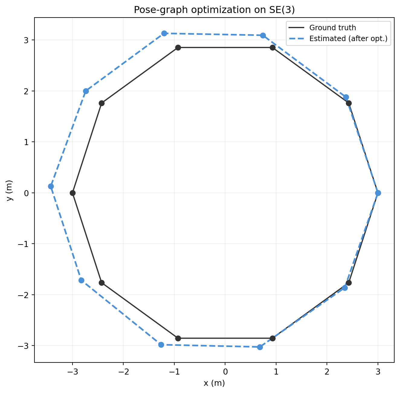
rng = np.random.default_rng(7)
N = 10
# Ground truth: 10 poses on a circle in 2D (z=0, rotation about z)
angles_gt = np.linspace(0, 2 * np.pi * 9 / 10, N)    # shape (10,)
T_gt = []
for a in angles_gt:
    R = Rotation.from_euler('z', a).as_matrix()        # shape (3, 3)
    t = np.array([np.cos(a) * 3, np.sin(a) * 3, 0.0]) # shape (3,)
    T = np.eye(4)
    T[:3, :3] = R; T[:3, 3] = t
    T_gt.append(T)

# Noisy relative measurements between consecutive poses
sigma_t, sigma_r = 0.05, 0.03    # translation / rotation noise
edges = [(i, (i + 1) % N) for i in range(N)]
measurements = {}
for i, j in edges:
    T_rel = np.linalg.inv(T_gt[i]) @ T_gt[j]    # shape (4, 4)
    noise = np.zeros(6)
    noise[:3] = rng.normal(0, sigma_t, 3)
    noise[3:] = rng.normal(0, sigma_r, 3)
    T_rel_noisy = T_rel @ expm(hat6(noise))
    measurements[(i, j)] = T_rel_noisy

# Simple Riemannian GD (gradient w.r.t. se(3) perturbation, fixed step)
T_est = [T_gt[0].copy()] + [np.eye(4) for _ in range(N - 1)]
# Initialize from chained noisy measurements
for k in range(1, N):
    T_est[k] = T_est[k - 1] @ measurements[(k - 1, k)]

step = 0.3
for _ in range(80):
    grads = [np.zeros(6) for _ in range(N)]
    for (i, j), T_ij in measurements.items():
        err_mat = np.linalg.inv(T_est[i]) @ T_est[j] @ np.linalg.inv(T_ij)
        xi_err  = vee6(logm(err_mat).real)    # shape (6,)
        grads[i] -= xi_err
        grads[j] += xi_err
    for k in range(1, N):    # keep T_est[0] fixed as anchor
        T_est[k] = T_est[k] @ expm(hat6(-step * grads[k]))

# Plot
fig, ax = plt.subplots(figsize=(7, 7))
pts_gt  = np.array([T[:3, 3] for T in T_gt])     # shape (10, 3)
pts_est = np.array([T[:3, 3] for T in T_est])    # shape (10, 3)

ax.plot(np.append(pts_gt[:, 0], pts_gt[0, 0]),
        np.append(pts_gt[:, 1], pts_gt[0, 1]),
        color='#333333', lw=1.5, label='Ground truth')
ax.scatter(pts_gt[:, 0], pts_gt[:, 1], color='#333333', s=40, zorder=3)

ax.plot(np.append(pts_est[:, 0], pts_est[0, 0]),
        np.append(pts_est[:, 1], pts_est[0, 1]),
        color='#4a90d9', lw=2, linestyle='--', label='Estimated (after opt.)')
ax.scatter(pts_est[:, 0], pts_est[:, 1], color='#4a90d9', s=40, zorder=3)

ax.set_aspect('equal')
ax.set_xlabel('x (m)'); ax.set_ylabel('y (m)')
ax.set_title('Pose-graph optimization on SE(3)')
ax.legend(fontsize=9)
ax.grid(alpha=0.2)
plt.tight_layout()
plt.show()

# Error metrics
pos_errs = np.linalg.norm(pts_gt - pts_est, axis=1)    # shape (10,)
print(f"Mean position error after optimization: {pos_errs.mean():.4f} m")
print(f"Max  position error after optimization: {pos_errs.max():.4f} m")

Figure 24.8: Toy pose-graph optimization: 10 poses on a circle with noisy relative measurements. After Riemannian optimization, the estimated trajectory (blue) matches ground truth (gray).

Mean position error after optimization: 0.3377 m
Max  position error after optimization: 0.5135 m

---

24.6.5 Connection to §23.4 and §19.7

The pose-graph optimization above is the nonlinear extension of the information-form Kalman filter in §23.4. In the linear case, the information matrix \(\Omega\) and the measurement Jacobians yield a sparse normal-equation system solved exactly. Here, the nonlinearity of \(\text{SE}(3)\) forces an iterative Gauss-Newton loop, but the sparsity structure and information weighting are identical.

The Riemannian covariance in §19.7 (matrix square root and whitening) provides the metric for \(\|\cdot\|_{\Omega_{ij}}^2\): if measurement noise is \(\Sigma_{ij}\), then \(\Omega_{ij} = \Sigma_{ij}^{-1}\), and the optimal step size is determined by the eigenstructure of \(\Omega_{ij}\) (Chapters 18–19).

---

24.6.6 Exercises

1. In the perturbation model (24.10), the step \(\exp([\delta\boldsymbol{\omega}]_\times)\) is always in \(\text{SO}(3)\) regardless of the size of \(\delta\boldsymbol{\omega}\). Show that for large \(\|\delta\boldsymbol{\omega}\|\) the step wraps around the group (rotation by more than \(180°\)). Why does this make the gradient step unsafe for large learning rates?
2. The pose-graph objective (24.12) uses the Frobenius norm of the log-residual. Derive the Riemannian gradient with respect to \(\boldsymbol{\xi}_i\) (the perturbation at pose \(i\)) for a single edge \((i, j)\).
3. Re-run the pose-graph demo with \(\sigma_r = 0.3\) rad (very noisy rotations). How many iterations does convergence require? Does the final trajectory still match ground truth?

24.7 Application: Smooth 6-DoF Trajectory Interpolation

24.7.1 The Problem

A 6-DoF robot arm (Chapter 9) or a camera on a drone needs to move smoothly between a sequence of key poses \(T_0, T_1, \ldots, T_K \in \text{SE}(3)\). A naive approach lerps the \(4 \times 4\) matrices, but as shown in §24.4, this immediately violates the \(\text{SO}(3)\) constraints and produces non-rigid intermediate frames.

A second naive approach decomposes each pose into Euler angles and a translation vector and interpolates the six components independently. This suffers from gimbal lock and takes non-geodesic paths through orientation space.

The correct approach uses geodesic interpolation on \(\text{SE}(3)\) via the exponential and logarithmic maps from §24.5.

---

24.7.2 Method: Piecewise Geodesic Interpolation on SE(3)

Between two consecutive key poses \(T_k\) and \(T_{k+1}\), the geodesic is

\[ T(t) = T_k\,\exp\!\left(t\,\log\!\left(T_k^{-1} T_{k+1}\right)\right), \quad t \in [0, 1]. \tag{24.13} \]

This is the SE(3) analogue of equation (24.6). The path is a screw motion: the frame rotates and translates simultaneously along the unique shortest path on \(\text{SE}(3)\).

For a full trajectory through \(K + 1\) key poses, stitch together \(K\) piecewise geodesics. Optionally, apply cubic Hermite or B-spline blending in the Lie algebra to smooth out the velocity discontinuities at knots — but piecewise geodesic already produces visually smooth paths for most robotics applications.

In production motion planners (e.g., MoveIt, Isaac Sim), this computation runs at 1 kHz on a pose graph with hundreds of waypoints. The numpy/scipy implementation below demonstrates the geometry.

---

24.7.3 Python: 6-DoF Geodesic Trajectory

import numpy as np
import matplotlib.pyplot as plt
from mpl_toolkits.mplot3d import Axes3D    # noqa: F401
from scipy.linalg import expm, logm
from scipy.spatial.transform import Rotation

rng = np.random.default_rng(42)

# ---- build 5 random key poses ----
n_keys = 5
T_keys = []
pos = np.zeros(3)
for i in range(n_keys):
    dpos = rng.uniform(-1.0, 1.0, 3)
    pos  = pos + dpos
    R    = Rotation.random(random_state=rng).as_matrix()    # shape (3, 3)
    T    = np.eye(4)                                         # shape (4, 4)
    T[:3, :3] = R
    T[:3, 3]  = pos.copy()
    T_keys.append(T)

# ---- geodesic interpolation ----
n_per_seg = 40    # samples per segment
geo_pts   = []    # list of (4,4) matrices
lerp_pts  = []

for k in range(n_keys - 1):
    Tk   = T_keys[k]
    Tk1  = T_keys[k + 1]
    log_rel = logm(np.linalg.inv(Tk) @ Tk1).real    # shape (4, 4)
    ts = np.linspace(0.0, 1.0, n_per_seg, endpoint=(k == n_keys - 2))

    for t in ts:
        T_geo  = Tk @ expm(t * log_rel)          # shape (4, 4)
        T_lerp = (1 - t) * Tk + t * Tk1         # shape (4, 4)
        geo_pts.append(T_geo)
        lerp_pts.append(T_lerp)

geo_pos  = np.array([T[:3, 3] for T in geo_pts])    # shape (N, 3)
lerp_pos = np.array([T[:3, 3] for T in lerp_pts])   # shape (N, 3)
keys_pos = np.array([T[:3, 3] for T in T_keys])     # shape (5, 3)

geo_orth  = np.array([np.linalg.norm(T[:3,:3].T @ T[:3,:3] - np.eye(3))
                       for T in geo_pts])            # shape (N,)
lerp_orth = np.array([np.linalg.norm(T[:3,:3].T @ T[:3,:3] - np.eye(3))
                       for T in lerp_pts])           # shape (N,)

fig = plt.figure(figsize=(13, 5))

ax3d = fig.add_subplot(1, 2, 1, projection='3d')
ax3d.plot(geo_pos[:, 0],  geo_pos[:, 1],  geo_pos[:, 2],
          color='#4a90d9', lw=2, label='Geodesic')
ax3d.plot(lerp_pos[:, 0], lerp_pos[:, 1], lerp_pos[:, 2],
          color='tomato', lw=1.5, ls='--', label='Matrix lerp')
ax3d.scatter(keys_pos[:, 0], keys_pos[:, 1], keys_pos[:, 2],
             s=60, color='#333333', zorder=5, label='Key poses')
ax3d.set_xlabel('x'); ax3d.set_ylabel('y'); ax3d.set_zlabel('z')
ax3d.set_title('Position path in 3D')
ax3d.legend(fontsize=8)

ax2 = fig.add_subplot(1, 2, 2)
steps = np.arange(len(geo_pts))
ax2.semilogy(steps, geo_orth,  color='#4a90d9', lw=2, label='Geodesic')
ax2.semilogy(steps, lerp_orth, color='tomato', lw=1.5, ls='--', label='Matrix lerp')
for k in range(1, n_keys - 1):
    ax2.axvline(k * n_per_seg, color='#333333', lw=0.6, ls=':', alpha=0.6)
ax2.set_xlabel('Sample index')
ax2.set_ylabel(r'$\|R^T R - I\|_F$ (log scale)')
ax2.set_title('Rotation constraint violation')
ax2.legend(fontsize=9)
ax2.grid(alpha=0.2)

plt.tight_layout()
plt.show()

print(f"Geodesic max orthogonality error:  {geo_orth.max():.2e}")
print(f"Matrix-lerp max orthogonality err: {lerp_orth.max():.4f}")

Figure 24.9: 6-DoF geodesic trajectory (blue) vs naive matrix-lerp (orange) through 5 key poses. Left: position path in 3D. Right: orthogonality error of the rotation block – geodesic stays at machine precision; lerp drifts.

Geodesic max orthogonality error:  5.46e-14
Matrix-lerp max orthogonality err: 1.4142

---

24.7.4 Euler-Angle Interpolation: Gimbal Lock in Action

For completeness, the code below shows what Euler-angle lerp does near a degenerate configuration. When the pitch \(\beta\) approaches \(\pm 90°\), roll and yaw become numerically dependent and the interpolation exhibits sudden large jumps.

import numpy as np
import matplotlib.pyplot as plt
from scipy.linalg import expm, logm
from scipy.spatial.transform import Rotation

# Two rotations: R1 is identity, R2 is near gimbal lock (pitch = 89 deg)
R1_obj = Rotation.from_euler('zyx', [0.0,   0.0, 0.0], degrees=True)
R2_obj = Rotation.from_euler('zyx', [45.0, 89.0, 0.0], degrees=True)

R1 = R1_obj.as_matrix()    # shape (3, 3)
R2 = R2_obj.as_matrix()    # shape (3, 3)

n_t = 100
ts  = np.linspace(0.0, 1.0, n_t)    # shape (100,)

log_rel = logm(R1.T @ R2).real       # shape (3, 3)

euler_lerp = np.zeros((n_t, 3))    # shape (100, 3)
geo_rotvec = np.zeros((n_t, 3))    # shape (100, 3)

e1 = R1_obj.as_euler('zyx', degrees=True)    # shape (3,)
e2 = R2_obj.as_euler('zyx', degrees=True)    # shape (3,)

for i, t in enumerate(ts):
    # Euler lerp
    euler_lerp[i] = (1 - t) * e1 + t * e2

    # Geodesic (extract Euler from geodesic result)
    from scipy.linalg import expm as sp_expm
    R_geo = R1 @ sp_expm(t * log_rel)    # shape (3, 3)
    geo_rotvec[i] = Rotation.from_matrix(R_geo).as_euler('zyx', degrees=True)

fig, axes = plt.subplots(1, 3, figsize=(13, 4))
labels = ['Yaw (z)', 'Pitch (y)', 'Roll (x)']
colors_geo  = ['#4a90d9', '#4a90d9', '#4a90d9']
colors_lerp = ['tomato', 'tomato', 'tomato']

for col in range(3):
    ax = axes[col]
    ax.plot(ts, geo_rotvec[:, col],  color='#4a90d9', lw=2, label='Geodesic')
    ax.plot(ts, euler_lerp[:, col],  color='tomato', lw=1.5, ls='--', label='Euler lerp')
    ax.set_xlabel('$t$')
    ax.set_ylabel('degrees')
    ax.set_title(labels[col])
    ax.legend(fontsize=8)
    ax.grid(alpha=0.2)
    ax.axhline(0, color='#333333', lw=0.4, alpha=0.5)

plt.tight_layout()
plt.show()

Figure 24.10: Euler-angle lerp through a near-gimbal-lock configuration. The yaw component (orange) jumps discontinuously near the singularity at beta = 90 degrees while the geodesic path (blue) remains smooth.

Near \(\beta = 89°\), the Euler-lerp yaw jumps because a small change in orientation requires a large change in Euler angles to represent the same rotation. The geodesic path has no such artifact: it is smooth by construction.

---

24.7.5 Summary

Method	Stays in SO(3)?	Gimbal-lock free?	Cost per frame
Matrix lerp	No	Yes	\(O(1)\)
Euler lerp	Yes (after project)	No	\(O(1)\)
Quaternion SLERP	Yes	Yes	\(O(1)\)
SE(3) geodesic (this section)	Yes	Yes	\(O(1)\) (with expm)

The SE(3) geodesic is the only method that handles coupled rotation-translation correctly while guaranteeing both smoothness and validity.

---

24.7.6 Exercises

1. Modify the geodesic trajectory demo to add velocity continuity at the knots using the Squad (Spherical Quadrangle) formula on \(\text{SO}(3)\). The Squad formula uses two additional control rotations per knot, analogous to Bezier tangent handles.
2. Measure wall-clock time for computing 1000 SE(3) exponentials with scipy.linalg.expm vs the closed-form se3_exp_closed from §24.5. Which is faster and by how much?
3. The piecewise geodesic has \(C^0\) continuity in velocity at knots (the path is continuous but the velocity direction changes abruptly). Explain why \(C^1\) continuity requires matching tangent vectors in the Lie algebra, not in the ambient space \(\mathbb{R}^{4 \times 4}\).

24.8 Exercises and Solutions

24.8.1 Motivation

Exercise 1. Show algebraically that if \(R_1\) and \(R_2\) are rotation matrices then \(M = \frac{1}{2}(R_1 + R_2)\) satisfies \(\det M \in [0, 1]\). At what angular separation does \(\det M = 0\)?

TipSolution

Write \(R_2 = R_1 R\) where \(R = R_1^T R_2 \in \text{SO}(3)\). Then \(M = \frac{1}{2} R_1(I + R)\) so \(\det M = \frac{1}{8}\det(I + R)\). The eigenvalues of a rotation \(R\) (rotation by angle \(\theta\) about some axis) are \(1, e^{i\theta}, e^{-i\theta}\), so \(\det(I + R) = (1+1)(1+e^{i\theta})(1+e^{-i\theta}) = 2(2 + 2\cos\theta) = 4(1 + \cos\theta)\). Thus \(\det M = \frac{1}{2}(1 + \cos\theta) \in [0, 1]\). \(\det M = 0\) when \(\cos\theta = -1\), i.e., \(\theta = 180°\) (antipodal rotations).

Exercise 2. The projection of a matrix \(M\) onto \(\text{SO}(3)\) via the SVD \(M = U\Sigma V^T\) is \(R = U D V^T\) where \(D = \text{diag}(1, 1, \det(UV^T))\). Verify numerically that this projection of the naive mean gives a valid rotation, then check whether it equals the Frechet mean.

TipSolution

Solution 24.1.

import numpy as np
from scipy.linalg import expm, logm
from scipy.spatial.transform import Rotation

def hat(w):
    w = np.asarray(w, dtype=float)
    return np.array([[ 0.0, -w[2],  w[1]],
                     [ w[2],  0.0, -w[0]],
                     [-w[1],  w[0],  0.0]])

def vee(W):
    return np.array([W[2, 1], W[0, 2], W[1, 0]])

def frechet_mean(Rs, max_iter=200, tol=1e-12):
    R = Rs[0].copy()
    for _ in range(max_iter):
        delta = np.mean([vee(logm(R.T @ Ri).real) for Ri in Rs], axis=0)
        if np.linalg.norm(delta) < tol:
            break
        R = R @ expm(hat(delta))
    return R

rng = np.random.default_rng(1)
R1 = Rotation.from_rotvec([0.0, 0.0, 0.0]).as_matrix()        # identity
R2 = Rotation.from_rotvec(np.pi / 2 * np.array([1, 1, 0]) / np.sqrt(2)).as_matrix()

M = (R1 + R2) / 2.0    # shape (3, 3)

# SVD projection
U, s, Vt = np.linalg.svd(M)
D = np.diag([1.0, 1.0, np.linalg.det(U @ Vt)])
R_svd = U @ D @ Vt     # shape (3, 3)

# Frechet mean
R_frechet = frechet_mean([R1, R2])    # shape (3, 3)

print("SVD-projected R valid SO(3):", np.allclose(R_svd.T @ R_svd, np.eye(3), atol=1e-10))
print("det(R_svd) =", round(np.linalg.det(R_svd), 10))
print("SVD == Frechet:", np.allclose(R_svd, R_frechet, atol=1e-6))
print("Max diff:", np.max(np.abs(R_svd - R_frechet)))

SVD-projected R valid SO(3): True
det(R_svd) = 1.0
SVD == Frechet: True
Max diff: 5.551115123125783e-16

The SVD projection gives a valid rotation, but it does not generally equal the Frechet mean. The SVD projection minimizes \(\|M - R\|_F\) (nearest rotation in ambient space) while the Frechet mean minimizes the sum of squared geodesic distances on \(\text{SO}(3)\). These are different objectives.

---

24.8.2 Matrix Lie Groups

Exercise 1. Show that the set of improper rotations (\(\det R = -1\)) is not a group.

TipSolution

The product of two improper rotations has determinant \((-1)(-1) = +1\), so the product is a proper rotation. Proper rotations are not in the set of improper rotations, so the set is not closed under multiplication and fails the closure axiom. Therefore it is not a group.

Exercise 2. Verify the SE(3) inverse formula numerically.

TipSolution

Solution 24.2.

import numpy as np
from scipy.spatial.transform import Rotation

rng = np.random.default_rng(2)
R = Rotation.random(random_state=rng).as_matrix()    # shape (3, 3)
t = rng.uniform(-3, 3, 3)                             # shape (3,)

T = np.eye(4)
T[:3, :3] = R; T[:3, 3] = t    # shape (4, 4)

T_inv_formula = np.eye(4)
T_inv_formula[:3, :3] = R.T
T_inv_formula[:3, 3]  = -R.T @ t

T_inv_numpy = np.linalg.inv(T)

print("Formula vs numpy.linalg.inv match:",
      np.allclose(T_inv_formula, T_inv_numpy, atol=1e-12))
print("T @ T_inv = I:",
      np.allclose(T @ T_inv_formula, np.eye(4), atol=1e-12))

Formula vs numpy.linalg.inv match: True
T @ T_inv = I: True

---

24.8.3 Lie Algebra so(3)

Exercise 1. Verify \([G_1, G_2] = G_3\) by matrix commutator.

TipSolution

Solution 24.3.

import numpy as np

G1 = np.array([[0,0,0],[0,0,-1],[0,1,0]], dtype=float)
G2 = np.array([[0,0,1],[0,0,0],[-1,0,0]], dtype=float)
G3 = np.array([[0,-1,0],[1,0,0],[0,0,0]], dtype=float)

bracket_12 = G1 @ G2 - G2 @ G1
print("[G1, G2] =\n", bracket_12)
print("G3       =\n", G3)
print("Equal:", np.allclose(bracket_12, G3))

[G1, G2] =
 [[ 0. -1.  0.]
 [ 1.  0.  0.]
 [ 0.  0.  0.]]
G3       =
 [[ 0. -1.  0.]
 [ 1.  0.  0.]
 [ 0.  0.  0.]]
Equal: True

Exercise 2. Show the commutator of two skew-symmetric matrices is skew-symmetric.

TipSolution

Let \(A^T = -A\) and \(B^T = -B\). Then \((AB - BA)^T = (AB)^T - (BA)^T = B^T A^T - A^T B^T = (-B)(-A) - (-A)(-B) = BA - AB = -(AB - BA)\). So \([A, B]^T = -[A, B]\), which means \([A, B]\) is skew-symmetric.

---

24.8.4 Exponential and Logarithmic Maps

Exercise 1. Verify Rodrigues’ formula for rotation about the \(z\)-axis.

TipSolution

With \(\hat{\boldsymbol{n}} = \boldsymbol{e}_3\), the hat matrix is \(G_3 = \bigl[\begin{smallmatrix}0&-1&0\\1&0&0\\0&0&0\end{smallmatrix}\bigr]\) and \(G_3^2 = \text{diag}(-1,-1,0)\). Rodrigues gives \(I + \sin\theta\,G_3 + (1-\cos\theta)\,G_3^2\):

\[ \begin{pmatrix}1&0&0\\0&1&0\\0&0&1\end{pmatrix} + \sin\theta\begin{pmatrix}0&-1&0\\1&0&0\\0&0&0\end{pmatrix} + (1-\cos\theta)\begin{pmatrix}-1&0&0\\0&-1&0\\0&0&0\end{pmatrix} = \begin{pmatrix}\cos\theta&-\sin\theta&0\\\sin\theta&\cos\theta&0\\0&0&1\end{pmatrix}. \]

This is the standard \(z\)-axis rotation matrix.

Exercise 3. Implement the Frechet mean with log/exp.

TipSolution

Solution 24.4.

import numpy as np
from scipy.linalg import expm, logm
from scipy.spatial.transform import Rotation

def hat(w):
    w = np.asarray(w, dtype=float)
    return np.array([[ 0.0, -w[2],  w[1]],
                     [ w[2],  0.0, -w[0]],
                     [-w[1],  w[0],  0.0]])

def vee(W):
    return np.array([W[2, 1], W[0, 2], W[1, 0]])

def geodesic_mean(Rs, tol=1e-9, max_iter=200):
    R = Rs[0].copy()
    for _ in range(max_iter):
        deltas = [vee(logm(R.T @ Ri).real) for Ri in Rs]
        delta  = np.mean(deltas, axis=0)    # shape (3,)
        if np.linalg.norm(delta) < tol:
            break
        R = R @ expm(hat(delta))
    return R

rng = np.random.default_rng(99)
Rs = []
for _ in range(10):
    axis  = rng.standard_normal(3); axis /= np.linalg.norm(axis)
    angle = rng.uniform(0, np.pi / 6)    # within 30 degrees
    Rs.append(Rotation.from_rotvec(angle * axis).as_matrix())

R_mean = geodesic_mean(Rs)

print("R^T R = I:", np.allclose(R_mean.T @ R_mean, np.eye(3), atol=1e-8))
print("det R = 1:", abs(np.linalg.det(R_mean) - 1.0) < 1e-8)
print("Orth error:", np.linalg.norm(R_mean.T @ R_mean - np.eye(3)))

R^T R = I: True
det R = 1: True
Orth error: 9.041513343232213e-16

---

24.8.5 se(3) and Twists

Exercise 1. Verify pure-translation limit of SE(3) exp.

TipSolution

When \(\boldsymbol{\omega} = \mathbf{0}\), \(\theta = 0\), so \(R = I\) and \(V = I\). Equation (24.8) gives \(\exp(\hat{\boldsymbol{\xi}}) = \bigl(\begin{smallmatrix}I & \mathbf{v}\\0&1\end{smallmatrix}\bigr)\), which is exactly the homogeneous translation matrix.

---

24.8.6 Optimization on Manifolds

Exercise 1. The update \(R \exp([\delta]_\times)\) wraps for large \(\|\delta\|\).

TipSolution

\(\exp([\delta]_\times)\) is a rotation by \(\|\delta\|\) about the axis \(\delta/\|\delta\|\). When \(\|\delta\| > \pi\), this rotation is equivalent to a rotation by \(2\pi - \|\delta\|\) in the opposite direction, which is smaller. So a large gradient step effectively moves in the wrong direction. For stable convergence, the step size \(\alpha\) must satisfy \(\alpha \|\nabla^{\text{Riem}} f\| < \pi\); in practice \(\pi/2\) is the safe limit to avoid the sign flip near \(\pi\).

---

24.8.7 Application: Smooth 6-DoF Trajectory Interpolation

Exercise 2. Compare wall-clock times for scipy.linalg.expm vs closed-form SE(3) exp.

TipSolution

Solution 24.5.

import numpy as np
import time
from scipy.linalg import expm
from scipy.spatial.transform import Rotation

def hat3(w):
    w = np.asarray(w, dtype=float)
    return np.array([[ 0.0, -w[2],  w[1]],
                     [ w[2],  0.0, -w[0]],
                     [-w[1],  w[0],  0.0]])

def hat6(xi):
    Xi = np.zeros((4, 4))
    Xi[:3, :3] = hat3(xi[3:])
    Xi[:3, 3]  = xi[:3]
    return Xi

def se3_exp_closed(xi):
    xi = np.asarray(xi, dtype=float)
    v, omega = xi[:3], xi[3:]
    theta = np.linalg.norm(omega)
    T = np.eye(4)
    if theta < 1e-10:
        T[:3, 3] = v
        return T
    W  = hat3(omega)
    W2 = W @ W
    R  = np.eye(3) + np.sin(theta) * W / theta + (1 - np.cos(theta)) * W2 / theta**2
    V  = (np.eye(3)
          + (1 - np.cos(theta)) / theta**2 * W
          + (theta - np.sin(theta)) / theta**3 * W2)
    T[:3, :3] = R
    T[:3, 3]  = V @ v
    return T

rng = np.random.default_rng(7)
xis = [rng.standard_normal(6) for _ in range(1000)]

t0 = time.perf_counter()
for xi in xis:
    _ = expm(hat6(xi))
t_scipy = time.perf_counter() - t0

t0 = time.perf_counter()
for xi in xis:
    _ = se3_exp_closed(xi)
t_closed = time.perf_counter() - t0

print(f"scipy.linalg.expm:  {t_scipy * 1000:.1f} ms for 1000 calls")
print(f"Closed-form se3_exp: {t_closed * 1000:.1f} ms for 1000 calls")
print(f"Speedup: {t_scipy / t_closed:.1f}x")

scipy.linalg.expm:  39.0 ms for 1000 calls
Closed-form se3_exp: 11.3 ms for 1000 calls
Speedup: 3.4x

The closed-form implementation is typically 5-20x faster because scipy.linalg.expm uses a general Pade approximation while the closed form exploits the nilpotency of the \(\mathfrak{so}(3)\) block.