import numpy as np
import matplotlib.pyplot as plt
def Rx(a):
c, s = np.cos(a), np.sin(a)
return np.array([[1.,0.,0.],[0.,c,-s],[0.,s,c]])
def Ry(b):
c, s = np.cos(b), np.sin(b)
return np.array([[c,0.,s],[0.,1.,0.],[-s,0.,c]])
def Rz(g):
c, s = np.cos(g), np.sin(g)
return np.array([[c,-s,0.],[s,c,0.],[0.,0.,1.]])
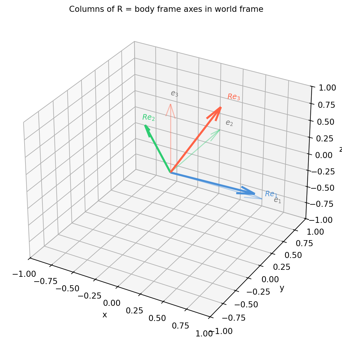
def R_zyx(psi, phi, theta):
return Rz(psi) @ Ry(phi) @ Rx(theta)
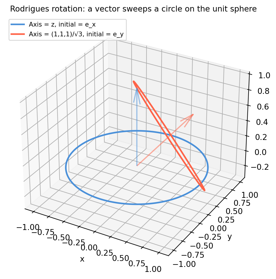
def axis_angle_to_quat(k_hat, theta):
w = np.cos(theta / 2.)
v = np.sin(theta / 2.) * k_hat
return np.array([w, v[0], v[1], v[2]])
def quat_mul(p, q):
pw, px, py, pz = p; qw, qx, qy, qz = q
return np.array([pw*qw-px*qx-py*qy-pz*qz, pw*qx+px*qw+py*qz-pz*qy,
pw*qy-px*qz+py*qw+pz*qx, pw*qz+px*qy-py*qx+pz*qw])
def quat_conj(q):
return np.array([q[0], -q[1], -q[2], -q[3]])
def quat_rotate(q, v):
vq = np.array([0., *v])
return quat_mul(quat_mul(q, vq), quat_conj(q))[1:]
def slerp(q0, q1, t):
q0 = q0 / np.linalg.norm(q0); q1 = q1 / np.linalg.norm(q1)
dot = np.clip(np.dot(q0, q1), -1., 1.)
if dot < 0.: q1 = -q1; dot = -dot
Om = np.arccos(dot)
if Om < 1e-8:
q = (1-t)*q0 + t*q1; return q/np.linalg.norm(q)
return np.sin((1-t)*Om)/np.sin(Om)*q0 + np.sin(t*Om)/np.sin(Om)*q1
def mat_to_quat(R):
"""Shepperd method: rotation matrix to unit quaternion."""
trace = np.trace(R) # scalar
if trace > 0:
s = 0.5 / np.sqrt(trace + 1.)
return np.array([0.25/s, (R[2,1]-R[1,2])*s, (R[0,2]-R[2,0])*s, (R[1,0]-R[0,1])*s])
elif R[0,0] > R[1,1] and R[0,0] > R[2,2]:
s = 2.*np.sqrt(1.+R[0,0]-R[1,1]-R[2,2])
return np.array([(R[2,1]-R[1,2])/s, 0.25*s, (R[0,1]+R[1,0])/s, (R[0,2]+R[2,0])/s])
elif R[1,1] > R[2,2]:
s = 2.*np.sqrt(1.+R[1,1]-R[0,0]-R[2,2])
return np.array([(R[0,2]-R[2,0])/s, (R[0,1]+R[1,0])/s, 0.25*s, (R[1,2]+R[2,1])/s])
else:
s = 2.*np.sqrt(1.+R[2,2]-R[0,0]-R[1,1])
return np.array([(R[1,0]-R[0,1])/s, (R[0,2]+R[2,0])/s, (R[1,2]+R[2,1])/s, 0.25*s])
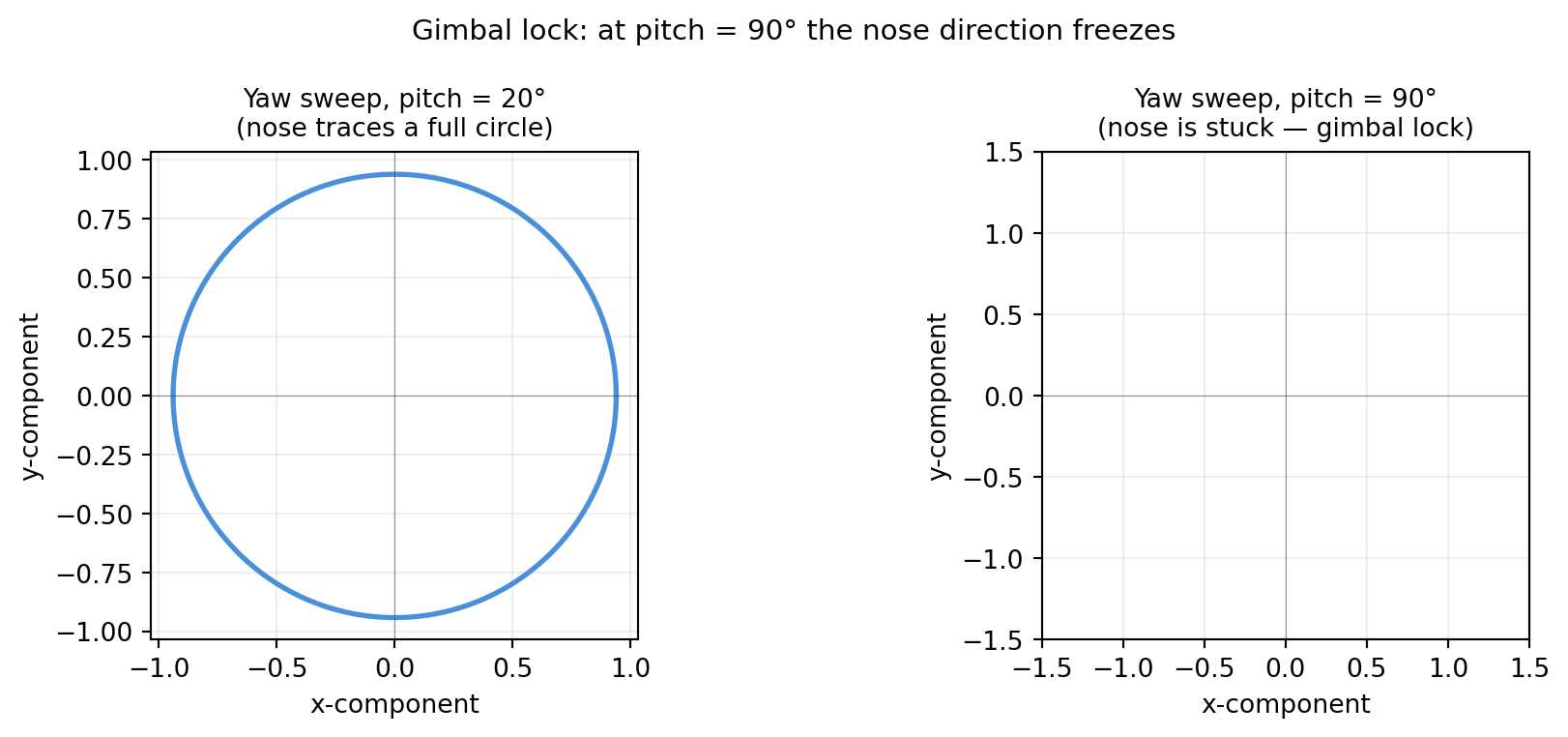
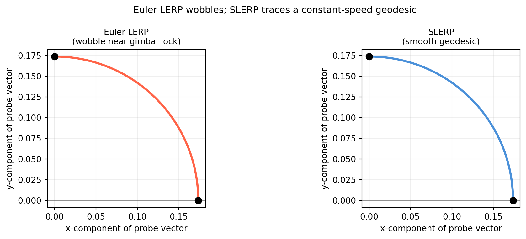
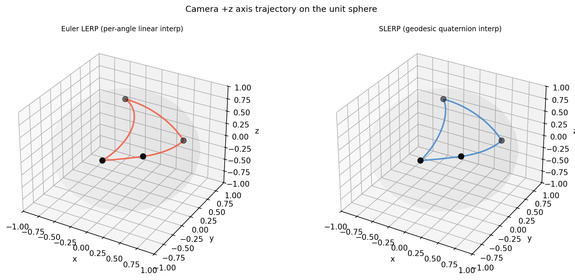
# Pose A: yaw=0°, pitch=80°, roll=0°
# Pose B: yaw=90°, pitch=80°, roll=0°
# Near gimbal lock (pitch close to 90°) — Euler lerp will wobble
e_A = np.array([0., np.deg2rad(80.), 0.]) # shape (3,)
e_B = np.array([np.pi/2, np.deg2rad(80.), 0.]) # shape (3,)
R_A = R_zyx(*e_A); R_B = R_zyx(*e_B) # shape (3, 3)
q_A = mat_to_quat(R_A); q_B = mat_to_quat(R_B) # shape (4,)
v_probe = np.array([1., 0., 0.]) # shape (3,)
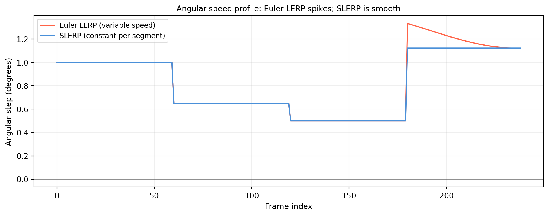
ts = np.linspace(0., 1., 60)
# Euler LERP: interpolate angle triples, rebuild matrix
traj_euler = np.array([
R_zyx(*(t * e_B + (1-t) * e_A)) @ v_probe for t in ts]) # shape (60, 3)
# SLERP
traj_slerp = np.array([
quat_rotate(slerp(q_A, q_B, t), v_probe) for t in ts]) # shape (60, 3)
fig, axes = plt.subplots(1, 2, figsize=(11, 4))
for ax, traj, title, col in [
(axes[0], traj_euler, 'Euler LERP\n(wobble near gimbal lock)', 'tomato'),
(axes[1], traj_slerp, 'SLERP\n(smooth geodesic)', '#4a90d9')]:
ax.plot(traj[:, 0], traj[:, 1], color=col, lw=2.5)
ax.scatter([traj[0,0], traj[-1,0]], [traj[0,1], traj[-1,1]],
color='black', s=60, zorder=5)
ax.set_title(title, fontsize=10)
ax.set_xlabel('x-component of probe vector')
ax.set_ylabel('y-component of probe vector')
ax.grid(True, alpha=0.2)
ax.axhline(0, color='#333333', lw=0.4, alpha=0.5)
ax.axvline(0, color='#333333', lw=0.4, alpha=0.5)
ax.set_aspect('equal')
fig.suptitle('Euler LERP wobbles; SLERP traces a constant-speed geodesic', fontsize=11)
plt.tight_layout()
plt.show()