11  Projective Geometry and Homography

11.1 Perspective Projection and Vanishing Points

The pinhole camera (§10.1) does something geometrically remarkable: it maps parallel lines to intersecting lines in the image. Those intersection points — called vanishing points — encode the direction of a set of parallel lines as a single image point. Understanding them requires extending ordinary Euclidean geometry with points at infinity.


11.1.1 Why Parallel Lines Converge

Consider two world-frame lines that run parallel to the \(X\)-axis:

\[\ell_1(s) = (s,\; 0,\; d_1),\quad \ell_2(s) = (s,\; 1,\; d_2)\]

Project each through a camera with \(f=1\), principal point at origin. The \(x\)-coordinate of the image point at parameter \(s\) is \(x = s/Z\). As \(s \to \infty\), both lines project to \(x \to \infty\) — but more precisely, the direction \((1, 0, 0)^T\) in world space maps to a fixed pixel called the vanishing point of that direction.

import numpy as np
import matplotlib.pyplot as plt

# Camera: identity extrinsic, f=400, principal point (320,240)
K = np.array([[400., 0., 320.],
              [  0.,400., 240.],
              [  0.,  0.,   1.]])   # shape (3, 3)

def project(pts_3d, K):
    """Project (N,3) points with intrinsic K. Returns (N,2) pixels."""
    p_h = (K @ pts_3d.T).T   # shape (N, 3)
    return p_h[:, :2] / p_h[:, 2:3]   # shape (N, 2)

# Three families of lines along x-axis, at different y and z offsets
s_vals = np.linspace(0.1, 30., 300)   # shape (300,)
families = [
    dict(dy=0., dz=3., color='#4a90d9'),
    dict(dy=0., dz=5., color='#2ecc71'),
    dict(dy=0., dz=7., color='tomato'),
    dict(dy=1., dz=3., color='#4a90d9'),
    dict(dy=1., dz=5., color='#2ecc71'),
    dict(dy=1., dz=7., color='tomato'),
    dict(dy=-1., dz=3., color='#4a90d9'),
    dict(dy=-1., dz=5., color='#2ecc71'),
    dict(dy=-1., dz=7., color='tomato'),
]

fig, ax = plt.subplots(figsize=(7, 5))
for fam in families:
    pts = np.column_stack([s_vals, np.full(300, fam['dy']), np.full(300, fam['dz'])])
    px = project(pts, K)
    ax.plot(px[:, 0], px[:, 1], color=fam['color'], lw=0.8, alpha=0.6)

# Vanishing point: direction (1,0,0) → project direction vector at Z→∞
# In practice: project a very far-away point
vp = project(np.array([[1e6, 0., 0.]]), K)
ax.scatter(vp[0, 0], vp[0, 1], color='black', s=80, zorder=5, label=f'Vanishing pt ({vp[0,0]:.0f}, {vp[0,1]:.0f})')

ax.set_xlim(200, 440); ax.set_ylim(180, 300)
ax.set_xlabel('u (px)'); ax.set_ylabel('v (px)')
ax.set_title('Lines Parallel to X-Axis Converge at Their Vanishing Point', fontsize=10)
ax.legend(fontsize=9)
ax.grid(True, alpha=0.2)
plt.tight_layout()
plt.show()
C:\Users\james.choi\AppData\Local\Temp\ipykernel_38040\1044232096.py:12: RuntimeWarning: divide by zero encountered in divide
  return p_h[:, :2] / p_h[:, 2:3]   # shape (N, 2)
C:\Users\james.choi\AppData\Local\Temp\ipykernel_38040\1044232096.py:12: RuntimeWarning: invalid value encountered in divide
  return p_h[:, :2] / p_h[:, 2:3]   # shape (N, 2)


11.1.2 The Projective Plane \(\mathbb{P}^2\)

In standard Euclidean geometry, two distinct parallel lines never meet. In projective geometry we add one “point at infinity” per direction so that every pair of distinct lines meets at exactly one point.

A homogeneous point in \(\mathbb{P}^2\) is a non-zero triple \((x, y, w)^T\) where \((x, y, w) \sim (\lambda x, \lambda y, \lambda w)\) for any \(\lambda \neq 0\).

Condition Interpretation
\(w \neq 0\) Ordinary point \(\left(\tfrac{x}{w},\, \tfrac{y}{w}\right) \in \mathbb{R}^2\)
\(w = 0\) Point at infinity in direction \((x, y)^T\)
import numpy as np

# Ordinary points
p1 = np.array([2., 3., 1.])    # represents (2, 3)
p2 = np.array([6., 9., 3.])    # same point — (6/3, 9/3) = (2, 3)
print("Ordinary points:")
print(f"  p1 = {p1}  →  ({p1[0]/p1[2]:.2f}, {p1[1]/p1[2]:.2f})")
print(f"  p2 = {p2}  →  ({p2[0]/p2[2]:.2f}, {p2[1]/p2[2]:.2f})")
print(f"  Same? {np.allclose(p1[0]/p1[2], p2[0]/p2[2]) and np.allclose(p1[1]/p1[2], p2[1]/p2[2])}")

# Point at infinity — encodes a direction, not a location
p_inf = np.array([1., 0., 0.])   # "point at infinity" along x-axis
print(f"\nPoint at infinity:  {p_inf}  (w=0, direction along x-axis)")

# A line in P2 is also a homogeneous triple ℓ = (a, b, c): ax + by + c = 0
# The line y = 2x - 1  →  -2x + y + 1 = 0  →  ℓ = (-2, 1, 1)
line = np.array([-2., 1., 1.])    # shape (3,)
pt_on_line = np.array([1., 1., 1.])   # (1,1): -2+1+1 = 0 ✓
print(f"\nLine ℓ = {line} (encodes -2x + y + 1 = 0)")
print(f"  Point (1,1) on line?  ℓ · p = {line @ pt_on_line:.4f}  (should be 0)")

# Intersection of two lines
l1 = np.array([-2., 1., 1.])   # y = 2x - 1
l2 = np.array([-1., 1., 3.])   # y = x - 3
# Intersection = cross product of line homogeneous vectors
x_meet = np.cross(l1, l2)          # shape (3,)
x_meet_euclid = x_meet[:2] / x_meet[2]
print(f"\nIntersection of l1 and l2:")
print(f"  Cross product: {x_meet}")
print(f"  Euclidean:     ({x_meet_euclid[0]:.4f}, {x_meet_euclid[1]:.4f})")
Ordinary points:
  p1 = [2. 3. 1.]  →  (2.00, 3.00)
  p2 = [6. 9. 3.]  →  (2.00, 3.00)
  Same? True

Point at infinity:  [1. 0. 0.]  (w=0, direction along x-axis)

Line ℓ = [-2.  1.  1.] (encodes -2x + y + 1 = 0)
  Point (1,1) on line?  ℓ · p = 0.0000  (should be 0)

Intersection of l1 and l2:
  Cross product: [ 2.  5. -1.]
  Euclidean:     (-2.0000, -5.0000)

11.1.3 Vanishing Points from Parallel Line Pairs

Given two parallel line pairs in an image (e.g., edges of a road), we can compute their vanishing point as the intersection of two image lines. In homogeneous coordinates, intersection = cross product.

import numpy as np
import matplotlib.pyplot as plt

def line_from_two_points(p1, p2):
    """Homogeneous line through two 2D points (given as homogeneous)."""
    return np.cross(p1, p2)   # shape (3,)

def intersect_lines(l1, l2):
    """Intersection of two homogeneous lines."""
    x = np.cross(l1, l2)   # shape (3,)
    return x / x[2]         # normalize so w=1

# Two pairs of parallel lines (pixel coords), e.g. road lane markings
# Left pair: converges to vanishing point V1
# Right pair: converges to same vanishing point (same direction)
left_line_pts  = [(np.array([100.,450.,1.]), np.array([280.,250.,1.])),
                  (np.array([200.,450.,1.]), np.array([310.,250.,1.]))]

right_line_pts = [(np.array([440.,450.,1.]), np.array([350.,250.,1.])),
                  (np.array([540.,450.,1.]), np.array([380.,250.,1.]))]

vp_candidates = []
for (a, b), (c, d) in [left_line_pts, right_line_pts]:
    l = line_from_two_points(a, b)   # shape (3,)
    m = line_from_two_points(c, d)   # shape (3,)
    vp_candidates.append(intersect_lines(l, m))

vp1 = vp_candidates[0]
vp2 = vp_candidates[1]
print(f"Vanishing point 1 (left pair):  ({vp1[0]:.1f}, {vp1[1]:.1f})")
print(f"Vanishing point 2 (right pair): ({vp2[0]:.1f}, {vp2[1]:.1f})")

fig, ax = plt.subplots(figsize=(7, 5))
colors = ['#4a90d9', '#2ecc71']
for idx, ((a, b), (c, d)) in enumerate([(left_line_pts[0], left_line_pts[1]),
                                         (right_line_pts[0], right_line_pts[1])]):
    for (p, q) in [(a, b), (c, d)]:
        ax.plot([p[0], q[0]], [p[1], q[1]], color=colors[idx], lw=2)
    vp = vp_candidates[idx]
    if 0 < vp[0] < 640 and 0 < vp[1] < 480:
        ax.scatter(vp[0], vp[1], s=120, color=colors[idx], zorder=5,
                   label=f'VP ({vp[0]:.0f}, {vp[1]:.0f})', marker='*')

ax.set_xlim(0, 640); ax.set_ylim(480, 0)
ax.set_xlabel('u (px)'); ax.set_ylabel('v (px)')
ax.set_title('Vanishing Points from Parallel Line Pairs', fontsize=10)
ax.legend(fontsize=9)
ax.grid(True, alpha=0.2)
plt.tight_layout()
plt.show()
Vanishing point 1 (left pair):  (357.1, 164.3)
Vanishing point 2 (right pair): (311.4, 164.3)


11.1.4 The Horizon Line

Two independent vanishing points define the horizon line (the line at infinity \(\ell_\infty\)). For a camera looking at a flat ground plane, the horizon is the locus of all vanishing points of horizontal directions — it lies at the height of the camera in the image.

import numpy as np

# Vanishing points (in homogeneous pixel coords)
vp1 = np.array([320., 200., 1.])   # shape (3,) — VPs on horizon
vp2 = np.array([580., 195., 1.])   # shape (3,)

# Horizon line = line through the two vanishing points
horizon = np.cross(vp1, vp2)   # shape (3,)
horizon = horizon / np.linalg.norm(horizon[:2])   # normalise

print(f"Horizon line ℓ = {horizon.round(6)}")
print(f"  Passes through VP1?  ℓ·VP1 = {horizon @ vp1:.4f}  (≈ 0)")
print(f"  Passes through VP2?  ℓ·VP2 = {horizon @ vp2:.4f}  (≈ 0)")

# Evaluate the horizon: at u=0 and u=640, what is v?
u_vals = np.array([0., 640.])
# ax + by + c = 0  →  y = -(ax + c) / b
a, b, c = horizon
v_vals = -(a * u_vals + c) / b
print(f"\nHorizon line crosses image at:")
print(f"  u=  0:  v = {v_vals[0]:.1f}")
print(f"  u=640:  v = {v_vals[1]:.1f}")
print(f"  (Nearly flat — camera is approximately level)")
Horizon line ℓ = [ 1.92270000e-02  9.99815000e-01 -2.06115737e+02]
  Passes through VP1?  ℓ·VP1 = 0.0000  (≈ 0)
  Passes through VP2?  ℓ·VP2 = 0.0000  (≈ 0)

Horizon line crosses image at:
  u=  0:  v = 206.2
  u=640:  v = 193.8
  (Nearly flat — camera is approximately level)

11.2 The Homography Matrix \(H\)

A homography is the projective transformation that relates two images of the same planar surface. It is a 3×3 matrix defined only up to scale (8 degrees of freedom), and it captures rotation, translation, and perspective distortion in a single matrix multiply.


11.2.1 Why Homographies Arise

Consider a flat checkerboard in the world (\(Z_w = 0\)). The full projection \(P = K[R \mid \mathbf{t}]\) reduces to a 3×3 map because the third world coordinate is always zero:

\[\lambda \begin{pmatrix}u\\v\\1\end{pmatrix} = K[\mathbf{r}_1 \; \mathbf{r}_2 \; \mathbf{t}] \begin{pmatrix}X_w\\Y_w\\1\end{pmatrix} = H \begin{pmatrix}X_w\\Y_w\\1\end{pmatrix}\]

The same relationship holds between any two views of a plane: the second image is a projective transformation of the first.

import numpy as np

def Rx(a):
    c,s=np.cos(a),np.sin(a); return np.array([[1.,0.,0.],[0.,c,-s],[0.,s,c]])
def Rz(g):
    c,s=np.cos(g),np.sin(g); return np.array([[c,-s,0.],[s,c,0.],[0.,0.,1.]])

K = np.array([[600., 0., 320.],
              [  0.,600., 240.],
              [  0.,  0.,   1.]])   # shape (3, 3)

# Camera: tilted 20° about x, then 10° about z, looking at Z=0 plane
R = Rx(np.deg2rad(-20.)) @ Rz(np.deg2rad(10.))   # shape (3, 3)
cam_pos = np.array([0.1, 0.0, -0.8])
t = -R @ cam_pos   # shape (3,)

# Homography for Z=0 plane: H = K [r1, r2, t]
r1, r2 = R[:, 0], R[:, 1]
H = K @ np.column_stack([r1, r2, t])   # shape (3, 3)
H = H / H[2, 2]                         # normalise
print("Homography H  (3×3, defined up to scale):")
print(H.round(4))

# Verify against full projection P for Z=0 points
Rt = np.column_stack([R, t])
P = K @ Rt   # shape (3, 4)

pts_2d = np.array([[0., 0.], [0.09, 0.], [0.09, 0.09], [0., 0.09]])   # shape (4, 2)
print(f"\n{'World (X,Y)':>18}  {'via H':>20}  {'via P':>20}  {'match':>6}")
for X, Y in pts_2d:
    p_w2d = np.array([X, Y, 1.])           # shape (3,) — 2D homogeneous world
    p_h   = H @ p_w2d                       # shape (3,)
    u_H, v_H = p_h[0]/p_h[2], p_h[1]/p_h[2]

    p_w3d = np.array([X, Y, 0., 1.])       # shape (4,) — 3D homogeneous world
    p_P   = P @ p_w3d                       # shape (3,)
    u_P, v_P = p_P[0]/p_P[2], p_P[1]/p_P[2]

    ok = np.allclose([u_H, v_H], [u_P, v_P], atol=1e-4)
    print(f"  ({X:.2f}, {Y:.2f})  →  ({u_H:.1f}, {v_H:.1f})  ({u_P:.1f}, {v_P:.1f})  {ok}")
Homography H  (3×3, defined up to scale):
[[ 7.547639e+02 -2.797605e+02  2.420153e+02]
 [ 1.104031e+02  6.261270e+02  4.437488e+02]
 [-7.840000e-02 -4.445000e-01  1.000000e+00]]

       World (X,Y)                 via H                 via P   match
  (0.00, 0.00)  →  (242.0, 443.7)  (242.0, 443.7)  True
  (0.09, 0.00)  →  (312.1, 456.9)  (312.1, 456.9)  True
  (0.09, 0.09)  →  (298.8, 535.2)  (298.8, 535.2)  True
  (0.00, 0.09)  →  (225.9, 520.9)  (225.9, 520.9)  True

11.2.2 Degrees of Freedom

A 3×3 matrix has 9 entries, but \(H\) is defined only up to a non-zero scale factor, leaving 8 degrees of freedom. Geometrically, those 8 DoF encode:

DoF Transformation
2 Translation in the image plane
1 Rotation in the image plane
1 Isotropic scale
2 Anisotropic shear / aspect ratio
2 Projective distortion (the two “perspective” parameters)

Four point correspondences (8 equations for 8 unknowns) are sufficient to determine \(H\) uniquely.


11.2.3 Applying a Homography: Forward Mapping

To project a set of planar world points into a new camera view, apply \(H\) and divide by the third coordinate.

import numpy as np
import matplotlib.pyplot as plt

def Rx(a):
    c,s=np.cos(a),np.sin(a); return np.array([[1.,0.,0.],[0.,c,-s],[0.,s,c]])
def Rz(g):
    c,s=np.cos(g),np.sin(g); return np.array([[c,-s,0.],[s,c,0.],[0.,0.,1.]])

K = np.array([[600., 0., 320.],[0., 600., 240.],[0., 0., 1.]])

def make_H(K, R, cam_pos):
    t = -R @ cam_pos
    r1, r2 = R[:,0], R[:,1]
    H = K @ np.column_stack([r1, r2, t])
    return H / H[2, 2]   # shape (3, 3)

# 6×6 checkerboard corners in world (Z=0)
sq = 0.03
xs = np.arange(7) * sq; ys = np.arange(7) * sq
XX, YY = np.meshgrid(xs, ys)
pts_w = np.column_stack([XX.ravel(), YY.ravel(), np.ones(49)])   # shape (49, 3)

# Two different views
views = [
    (Rx(np.deg2rad(-15.)) @ Rz(np.deg2rad( 5.)), np.array([ 0.09, 0.09,-0.85])),
    (Rx(np.deg2rad(-30.)) @ Rz(np.deg2rad(-20.)), np.array([-0.05, 0.05,-0.90])),
]

fig, axes = plt.subplots(1, 2, figsize=(10, 4.5))
for ax, (R, cam_pos), col in zip(axes, views, ['#4a90d9', 'tomato']):
    H = make_H(K, R, cam_pos)   # shape (3, 3)
    proj = (H @ pts_w.T).T      # shape (49, 3)
    uvs = proj[:, :2] / proj[:, 2:3]   # shape (49, 2)
    # Reshape to grid and draw grid lines
    U = uvs[:, 0].reshape(7, 7); V = uvs[:, 1].reshape(7, 7)
    for i in range(7):
        ax.plot(U[i, :], V[i, :], color=col, lw=1.)
        ax.plot(U[:, i], V[:, i], color=col, lw=1.)
    ax.set_xlim(50, 590); ax.set_ylim(430, 50)
    ax.set_xlabel('u (px)'); ax.set_ylabel('v (px)')
    ax.set_aspect('equal'); ax.grid(True, alpha=0.2)

axes[0].set_title('View 1: slight tilt', fontsize=10)
axes[1].set_title('View 2: steep + rotated', fontsize=10)
fig.suptitle('6×6 Checkerboard through Two Homographies', fontsize=11)
plt.tight_layout()
plt.show()


11.2.4 Image-to-Image Homography

When we compute \(H\) from point correspondences (pixel pairs) rather than from a known camera, we get the direct image-to-image mapping:

\[\lambda \begin{pmatrix}u'\\v'\\1\end{pmatrix} = H \begin{pmatrix}u\\v\\1\end{pmatrix}\]

This is the form used in panoramic stitching, image rectification, and document de-warping. We will compute \(H\) from correspondences in §11.3.

import numpy as np

# Given 4 point correspondences (source → destination)
src = np.array([[100., 120.], [420., 105.], [435., 380.], [ 85., 395.]])   # shape (4, 2)
dst = np.array([[ 50.,  50.], [550.,  50.], [550., 430.], [ 50., 430.]])   # shape (4, 2)

# Build the DLT system (see §11.3 for full derivation)
def build_A(src, dst):
    """Build 2n×9 DLT matrix for homography estimation."""
    A = []
    for (x, y), (u, v) in zip(src, dst):
        A.append([-x, -y, -1,  0,  0,  0, u*x, u*y, u])
        A.append([ 0,  0,  0, -x, -y, -1, v*x, v*y, v])
    return np.array(A)   # shape (2n, 9)

A = build_A(src, dst)     # shape (8, 9)
_, _, Vt = np.linalg.svd(A)
h = Vt[-1, :]              # shape (9,) — null vector
H = h.reshape(3, 3)
H = H / H[2, 2]

print("Estimated H:")
print(H.round(4))

# Verify: apply H to each source point
print(f"\n{'src':>16}  {'H·src (predicted)':>22}  {'dst (target)':>22}")
for p_s, p_d in zip(src, dst):
    p_h = H @ np.array([*p_s, 1.])
    pred = p_h[:2] / p_h[2]
    print(f"  {p_s}  →  ({pred[0]:.1f}, {pred[1]:.1f})  vs  {p_d}")
Estimated H:
[[ 1.648000e+00  1.077000e-01 -1.254171e+02]
 [ 7.590000e-02  1.602600e+00 -1.475984e+02]
 [ 0.000000e+00  4.000000e-04  1.000000e+00]]

             src       H·src (predicted)            dst (target)
  [100. 120.]  →  (50.0, 50.0)  vs  [50. 50.]
  [420. 105.]  →  (550.0, 50.0)  vs  [550.  50.]
  [435. 380.]  →  (550.0, 430.0)  vs  [550. 430.]
  [ 85. 395.]  →  (50.0, 430.0)  vs  [ 50. 430.]

11.3 Direct Linear Transform (DLT)

The Direct Linear Transform (DLT) is the standard algorithm for computing a homography from point correspondences. Each correspondence contributes two linear equations in the 9 unknown entries of \(H\). With \(n \geq 4\) correspondences we get a \(2n \times 9\) system \(A\mathbf{h} = \mathbf{0}\), solved by SVD.


11.3.1 Deriving the DLT System

For a correspondence \((x_i, y_i) \mapsto (u_i, v_i)\) under homography \(H\):

\[\lambda_i \begin{pmatrix}u_i\\v_i\\1\end{pmatrix} = H \begin{pmatrix}x_i\\y_i\\1\end{pmatrix}\]

Expanding and eliminating \(\lambda_i\) (cross-product trick) gives two equations per point:

\[\begin{bmatrix} -x_i & -y_i & -1 & 0 & 0 & 0 & u_i x_i & u_i y_i & u_i \\ 0 & 0 & 0 & -x_i & -y_i & -1 & v_i x_i & v_i y_i & v_i \end{bmatrix} \mathbf{h} = \mathbf{0}\]

where \(\mathbf{h} = \mathrm{vec}(H)\) is the 9-vector of entries of \(H\) read row by row.

import numpy as np

def dlt_homography(src, dst):
    """
    Estimate 3×3 homography from n>=4 correspondences using DLT.
    src: shape (n, 2)  source points
    dst: shape (n, 2)  destination points
    Returns H: shape (3, 3), normalised so H[2,2]=1.
    """
    n = len(src)
    A = np.zeros((2*n, 9))   # shape (2n, 9)
    for i, ((x, y), (u, v)) in enumerate(zip(src, dst)):
        A[2*i  ] = [-x, -y, -1,  0,  0,  0, u*x, u*y, u]
        A[2*i+1] = [ 0,  0,  0, -x, -y, -1, v*x, v*y, v]
    _, _, Vt = np.linalg.svd(A)    # Vt shape (9, 9)
    h = Vt[-1, :]                   # shape (9,) — smallest singular vector
    H = h.reshape(3, 3)             # shape (3, 3)
    return H / H[2, 2]

# Example: map a tilted quadrilateral to a frontal rectangle
src = np.array([[110., 130.],
                [390., 105.],
                [410., 360.],
                [ 90., 385.]], dtype=float)   # shape (4, 2)

dst = np.array([[ 50.,  50.],
                [500.,  50.],
                [500., 400.],
                [ 50., 400.]], dtype=float)   # shape (4, 2)

H = dlt_homography(src, dst)
print("DLT-estimated H:")
print(H.round(4))

# Verify
print(f"\n{'src':>18}{'DLT prediction':>20}  {'dst':>18}  {'err (px)':>10}")
for p_s, p_d in zip(src, dst):
    p_h = H @ np.array([*p_s, 1.])
    pred = p_h[:2] / p_h[2]
    err  = np.linalg.norm(pred - p_d)
    print(f"  ({p_s[0]:.0f},{p_s[1]:.0f})  →  ({pred[0]:.1f},{pred[1]:.1f})  "
          f"vs ({p_d[0]:.0f},{p_d[1]:.0f})  err={err:.4f}")
DLT-estimated H:
[[ 1.793200e+00  1.710000e-01 -1.649142e+02]
 [ 1.589000e-01  1.753200e+00 -1.908318e+02]
 [ 1.000000e-04  6.000000e-04  1.000000e+00]]

               src  →        DLT prediction                 dst    err (px)
  (110,130)  →  (50.0,50.0)  vs (50,50)  err=0.0000
  (390,105)  →  (500.0,50.0)  vs (500,50)  err=0.0000
  (410,360)  →  (500.0,400.0)  vs (500,400)  err=0.0000
  (90,385)  →  (50.0,400.0)  vs (50,400)  err=0.0000

11.3.2 Why SVD?

The system \(A\mathbf{h} = \mathbf{0}\) is homogeneous — the trivial solution \(\mathbf{h} = \mathbf{0}\) is always valid but useless. We add the constraint \(\|\mathbf{h}\| = 1\), which turns it into:

\[\min_{\mathbf{h}} \|A\mathbf{h}\|^2 \quad \text{subject to} \quad \|\mathbf{h}\| = 1\]

The solution is the right singular vector of \(A\) corresponding to its smallest singular value (the last row of \(V^T\) in np.linalg.svd).

import numpy as np

# Show the singular values of A for a well-conditioned case
src = np.array([[110., 130.],[390., 105.],[410., 360.],[ 90., 385.]], dtype=float)
dst = np.array([[ 50.,  50.],[500.,  50.],[500., 400.],[ 50., 400.]], dtype=float)

A = np.zeros((8, 9))
for i, ((x,y),(u,v)) in enumerate(zip(src, dst)):
    A[2*i  ] = [-x,-y,-1, 0, 0, 0, u*x, u*y, u]
    A[2*i+1] = [ 0, 0, 0,-x,-y,-1, v*x, v*y, v]

U, s, Vt = np.linalg.svd(A)   # s shape (8,), Vt shape (9,9)

print("Singular values of A (should have one near zero):")
print(s.round(4))
print(f"\nSmallest singular value: {s[-1]:.2e}  (≈ 0 → consistent system)")
print(f"Condition number: {s[0]/s[-1]:.1f}")
Singular values of A (should have one near zero):
[4.15067909e+05 1.28506392e+05 6.94030700e+02 4.03859700e+02
 2.60043400e+02 1.44953100e+02 4.15006000e+01 6.43500000e-01]

Smallest singular value: 6.44e-01  (≈ 0 → consistent system)
Condition number: 645015.2

11.3.3 Normalisation: Why Raw DLT Fails

Raw DLT is numerically sensitive when pixel coordinates are large (e.g., 640×480). The matrix \(A\) has entries ranging from \(\sim 1\) to \(\sim 10^5\), making the SVD ill-conditioned.

Hartley normalisation (1997): before running DLT, transform both point sets so that their centroid is at the origin and their average distance from the origin is \(\sqrt{2}\). After computing \(H\), undo the normalisation:

\[H = T_{\text{dst}}^{-1} \; \hat{H} \; T_{\text{src}}\]

import numpy as np

def normalise_points(pts):
    """
    Isotropic normalisation: centroid → origin, mean distance → sqrt(2).
    pts: shape (n, 2)
    Returns (pts_norm, T) where T is the 3×3 normalisation transform.
    """
    centroid = pts.mean(axis=0)             # shape (2,)
    shifted  = pts - centroid               # shape (n, 2)
    scale    = np.sqrt(2.) / np.mean(np.linalg.norm(shifted, axis=1))
    T = np.array([[scale, 0.,    -scale*centroid[0]],
                  [0.,    scale, -scale*centroid[1]],
                  [0.,    0.,     1.               ]])   # shape (3, 3)
    pts_h = np.column_stack([pts, np.ones(len(pts))])   # shape (n, 3)
    pts_n = (T @ pts_h.T).T[:, :2]                      # shape (n, 2)
    return pts_n, T

def dlt_normalised(src, dst):
    """DLT with Hartley normalisation. Returns H: shape (3, 3)."""
    src_n, T_src = normalise_points(src)   # shape (n,2), (3,3)
    dst_n, T_dst = normalise_points(dst)   # shape (n,2), (3,3)

    n = len(src_n)
    A = np.zeros((2*n, 9))
    for i, ((x,y),(u,v)) in enumerate(zip(src_n, dst_n)):
        A[2*i  ] = [-x,-y,-1, 0, 0, 0, u*x, u*y, u]
        A[2*i+1] = [ 0, 0, 0,-x,-y,-1, v*x, v*y, v]

    _, _, Vt = np.linalg.svd(A)
    H_norm = Vt[-1].reshape(3, 3)
    H = np.linalg.solve(T_dst, H_norm @ T_src)   # denormalise
    return H / H[2, 2]

# Compare raw vs normalised on a realistic 640×480 scenario
rng = np.random.default_rng(7)

# Ground-truth H: moderate perspective
src_clean = np.array([[110., 130.],[390., 105.],[410., 360.],[ 90., 385.],
                       [250., 245.],[300., 135.],[380., 300.],[140., 280.]], dtype=float)
dst_clean = np.array([[ 50.,  50.],[500.,  50.],[500., 400.],[ 50., 400.],
                       [275., 225.],[350., 120.],[450., 330.],[ 90., 340.]], dtype=float)

# Add small pixel noise
noise = rng.normal(0., 0.5, src_clean.shape)   # shape (8, 2)
src_noisy = src_clean + noise

H_raw  = dlt_homography(src_noisy, dst_clean)
H_norm = dlt_normalised(src_noisy, dst_clean)

def reprojection_rms(H, src, dst):
    errs = []
    for p_s, p_d in zip(src, dst):
        p_h = H @ np.array([*p_s, 1.])
        pred = p_h[:2] / p_h[2]
        errs.append(np.linalg.norm(pred - p_d))
    return np.sqrt(np.mean(np.array(errs)**2))

print(f"RMS reprojection error:")
print(f"  Raw DLT:         {reprojection_rms(H_raw,  src_noisy, dst_clean):.4f} px")
print(f"  Normalised DLT:  {reprojection_rms(H_norm, src_noisy, dst_clean):.4f} px")
RMS reprojection error:
  Raw DLT:         34.3820 px
  Normalised DLT:  25.0500 px

11.3.4 DLT is the Same Machinery as Zhang’s Calibration

Notice that §10.4 (Zhang’s method) also built a system \(V\mathbf{b} = \mathbf{0}\) and solved it with SVD. The pattern is universal:

Problem Unknown System size Solved by
Homography from \(n\) points \(\mathbf{h}\) (9-vec) \(2n \times 9\) SVD
Zhang’s \(B\) matrix from \(n\) views \(\mathbf{b}\) (6-vec) \(2n \times 6\) SVD
Fundamental matrix (§25) \(\mathbf{f}\) (9-vec) \(n \times 9\) SVD

The recipe: stack linear constraints → take null vector of \(A\) via SVD → reshape and normalise.

11.4 RANSAC for Robust Estimation

Real feature matches contain outliers — mismatched point pairs caused by repetitive textures, occlusion, or descriptor ambiguity. A single outlier corrupts the entire DLT solution. RANSAC (Random Sample Consensus, Fischler & Bolles 1981) is the standard fix: repeatedly fit \(H\) to a minimal random sample (4 pairs), count how many remaining matches agree with it (“inliers”), and keep the best fit.


11.4.1 The RANSAC Loop

repeat N times:
    1. Draw 4 random correspondences (minimal sample)
    2. Fit H_candidate using DLT on those 4 pairs
    3. For each remaining correspondence:
           if reprojection error < threshold τ:  mark as inlier
    4. If |inliers| > best_so_far:  save H_candidate
return best H_candidate, refined with all its inliers

The number of iterations \(N\) needed to guarantee (with probability \(p\)) that at least one sample is all-inlier:

\[N = \frac{\log(1-p)}{\log\!\left(1-(1-\varepsilon)^s\right)}\]

where \(\varepsilon\) is the outlier fraction and \(s=4\) is the minimum sample size.

import numpy as np

def ransac_iterations(outlier_frac, min_sample=4, confidence=0.99):
    """
    Number of RANSAC iterations for given outlier fraction.
    outlier_frac: fraction of points that are outliers (0–1)
    min_sample:   minimum sample size (4 for homography)
    confidence:   desired probability of finding an all-inlier sample
    Returns N (int).
    """
    inlier_prob = (1. - outlier_frac) ** min_sample   # prob all 4 are inliers
    if inlier_prob < 1e-15:
        return int(1e9)
    N = np.log(1. - confidence) / np.log(1. - inlier_prob)
    return int(np.ceil(N))

print("RANSAC iteration count  (s=4, p=0.99):")
print(f"{'Outlier %':>12}  {'N iterations':>14}")
for eps in [0.10, 0.20, 0.30, 0.40, 0.50, 0.60]:
    N = ransac_iterations(eps)
    print(f"  {eps*100:5.0f}%        {N:>10d}")
RANSAC iteration count  (s=4, p=0.99):
   Outlier %    N iterations
     10%                 5
     20%                 9
     30%                17
     40%                34
     50%                72
     60%               178

11.4.2 Full RANSAC Implementation

import numpy as np

def dlt_homography(src, dst):
    """DLT homography estimate. src,dst: shape (n,2). Returns H: (3,3)."""
    n = len(src)
    A = np.zeros((2*n, 9))
    for i, ((x,y),(u,v)) in enumerate(zip(src, dst)):
        A[2*i  ] = [-x,-y,-1, 0, 0, 0, u*x, u*y, u]
        A[2*i+1] = [ 0, 0, 0,-x,-y,-1, v*x, v*y, v]
    _, _, Vt = np.linalg.svd(A)
    H = Vt[-1].reshape(3, 3)
    return H / H[2, 2]

def reproj_errors(H, src, dst):
    """Per-point reprojection errors. Returns shape (n,)."""
    n = len(src)
    src_h = np.column_stack([src, np.ones(n)])   # shape (n, 3)
    proj  = (H @ src_h.T).T                       # shape (n, 3)
    pred  = proj[:, :2] / proj[:, 2:3]            # shape (n, 2)
    return np.linalg.norm(pred - dst, axis=1)      # shape (n,)

def ransac_homography(src, dst, max_iter=500, threshold=3.0, rng=None):
    """
    RANSAC homography estimation.
    src, dst:   shape (n, 2)
    threshold:  inlier reprojection error in pixels
    Returns (H_best, inlier_mask): H shape (3,3), mask shape (n,) bool.
    """
    if rng is None:
        rng = np.random.default_rng(0)
    n = len(src)
    best_inliers = np.zeros(n, dtype=bool)
    best_count   = 0

    for _ in range(max_iter):
        idx   = rng.choice(n, size=4, replace=False)
        H_try = dlt_homography(src[idx], dst[idx])        # shape (3, 3)
        errs  = reproj_errors(H_try, src, dst)            # shape (n,)
        mask  = errs < threshold                          # shape (n,) bool

        if mask.sum() > best_count:
            best_count   = mask.sum()
            best_inliers = mask

    # Refit on all inliers
    H_final = dlt_homography(src[best_inliers], dst[best_inliers])
    return H_final, best_inliers

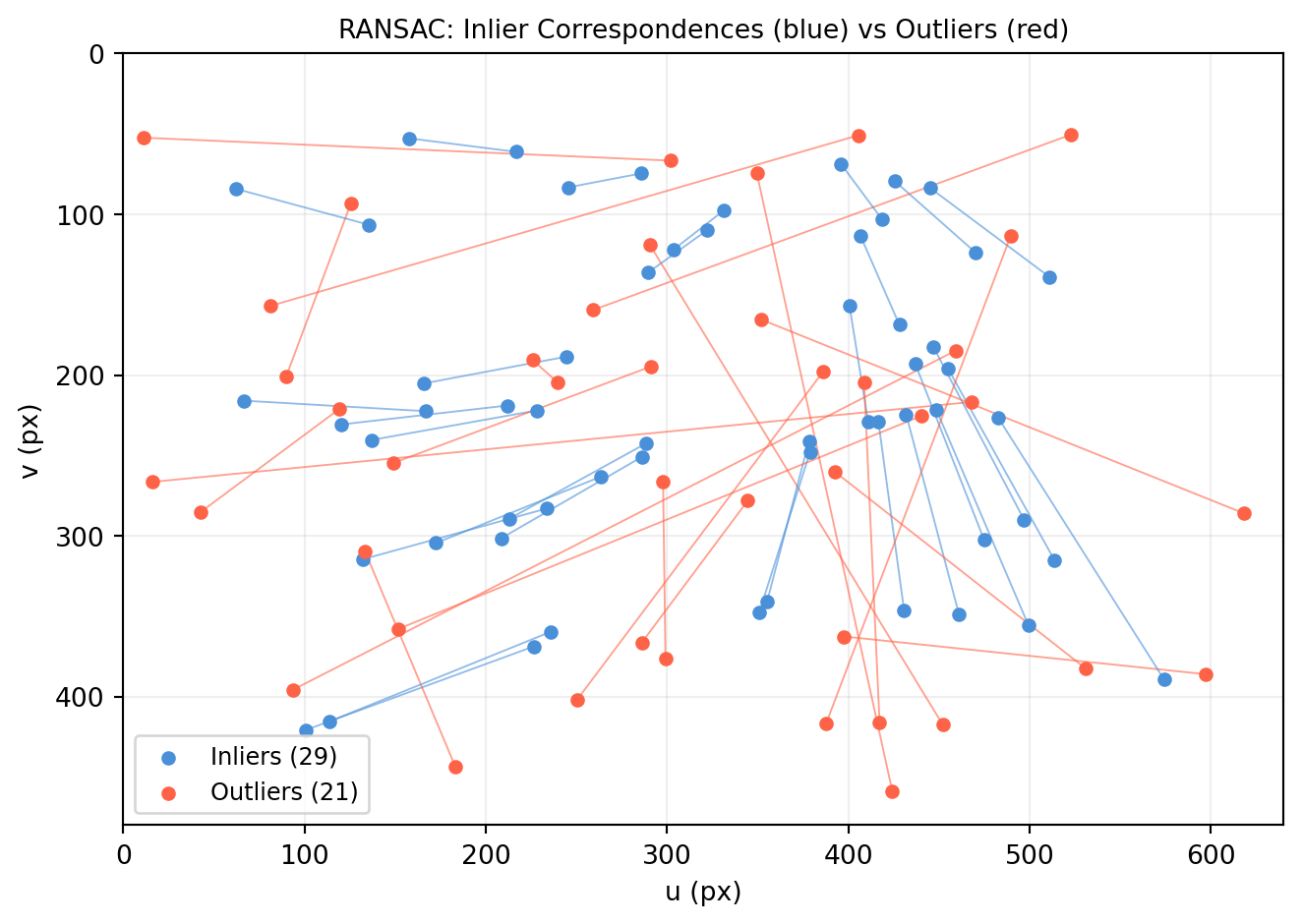
# --- Simulation: 50 matches, 40% outliers ---
rng = np.random.default_rng(42)

# Ground-truth H
H_true = np.array([[ 1.2, 0.3, 50.],
                   [-0.1, 1.1, 30.],
                   [ 0.001, 0.0005, 1.]])   # shape (3, 3)
H_true /= H_true[2, 2]

# Generate 50 source points (random pixel locations)
n_pts   = 50
src_all = rng.uniform([50., 50.], [590., 430.], (n_pts, 2))   # shape (50, 2)

# True destination points
src_h   = np.column_stack([src_all, np.ones(n_pts)])
proj    = (H_true @ src_h.T).T
dst_all = proj[:, :2] / proj[:, 2:3]   # shape (50, 2)

# Add small inlier noise
inlier_noise = rng.normal(0., 1.0, (n_pts, 2))   # shape (50, 2)
dst_all += inlier_noise

# Corrupt 40% of matches with random outliers
n_outliers = int(0.4 * n_pts)
outlier_idx = rng.choice(n_pts, size=n_outliers, replace=False)
dst_all[outlier_idx] = rng.uniform([0., 0.], [640., 480.], (n_outliers, 2))

# Run plain DLT (no RANSAC) and RANSAC
H_dlt, _  = np.linalg.svd(  # DLT on all points
    np.vstack([[-x,-y,-1,0,0,0,u*x,u*y,u] for (x,y),(u,v) in zip(src_all, dst_all)]
            + [[0,0,0,-x,-y,-1,v*x,v*y,v] for (x,y),(u,v) in zip(src_all, dst_all)])), 2
A = np.zeros((2*n_pts, 9))
for i, ((x,y),(u,v)) in enumerate(zip(src_all, dst_all)):
    A[2*i  ] = [-x,-y,-1, 0, 0, 0, u*x, u*y, u]
    A[2*i+1] = [ 0, 0, 0,-x,-y,-1, v*x, v*y, v]
_, _, Vt = np.linalg.svd(A)
H_dlt = Vt[-1].reshape(3, 3); H_dlt /= H_dlt[2,2]

H_ransac, inlier_mask = ransac_homography(src_all, dst_all, max_iter=500,
                                          threshold=3.0, rng=rng)

def rms_on_inliers(H, src, dst, mask):
    errs = reproj_errors(H, src[mask], dst[mask])
    return np.sqrt(np.mean(errs**2))

print(f"Points: {n_pts}  |  Outliers: {n_outliers} ({100*n_outliers/n_pts:.0f}%)")
print(f"Plain DLT  — RMS error (inliers only): "
      f"{rms_on_inliers(H_dlt,   src_all, dst_all, ~np.isin(np.arange(n_pts), outlier_idx)):.2f} px")
print(f"RANSAC     — inliers found: {inlier_mask.sum()}/{n_pts}")
print(f"           — RMS error (inliers only): "
      f"{rms_on_inliers(H_ransac, src_all, dst_all, ~np.isin(np.arange(n_pts), outlier_idx)):.2f} px")
Points: 50  |  Outliers: 20 (40%)
Plain DLT  — RMS error (inliers only): 3249.56 px
RANSAC     — inliers found: 29/50
           — RMS error (inliers only): 1.38 px

11.4.3 Visualising RANSAC Inliers vs Outliers

import numpy as np
import matplotlib.pyplot as plt

def dlt_homography(src, dst):
    n = len(src); A = np.zeros((2*n, 9))
    for i,((x,y),(u,v)) in enumerate(zip(src,dst)):
        A[2*i  ]=[-x,-y,-1,0,0,0,u*x,u*y,u]; A[2*i+1]=[0,0,0,-x,-y,-1,v*x,v*y,v]
    _,_,Vt=np.linalg.svd(A); H=Vt[-1].reshape(3,3); return H/H[2,2]

def reproj_errors(H, src, dst):
    sh=np.column_stack([src,np.ones(len(src))]); p=(H@sh.T).T
    return np.linalg.norm(p[:,:2]/p[:,2:3]-dst,axis=1)

def ransac_homography(src, dst, max_iter=500, threshold=3.0, rng=None):
    if rng is None: rng=np.random.default_rng(0)
    n=len(src); best=np.zeros(n,dtype=bool); best_c=0
    for _ in range(max_iter):
        idx=rng.choice(n,size=4,replace=False)
        try: H=dlt_homography(src[idx],dst[idx])
        except: continue
        mask=reproj_errors(H,src,dst)<threshold
        if mask.sum()>best_c: best_c=mask.sum(); best=mask
    return dlt_homography(src[best],dst[best]), best

rng = np.random.default_rng(42)
H_true = np.array([[1.2,0.3,50.],[-0.1,1.1,30.],[0.001,0.0005,1.]])
H_true /= H_true[2,2]
n_pts = 50
src_all = rng.uniform([50.,50.],[590.,430.],(n_pts,2))
src_h   = np.column_stack([src_all,np.ones(n_pts)])
proj    = (H_true@src_h.T).T; dst_all = proj[:,:2]/proj[:,2:3]
dst_all += rng.normal(0.,1.,(n_pts,2))
n_out = int(0.4*n_pts); oidx = rng.choice(n_pts,size=n_out,replace=False)
dst_all[oidx] = rng.uniform([0.,0.],[640.,480.],(n_out,2))

_, mask = ransac_homography(src_all, dst_all, rng=rng)

fig, ax = plt.subplots(figsize=(7, 5))
# Draw lines for each correspondence (source → destination)
for i, (s, d) in enumerate(zip(src_all, dst_all)):
    col = '#4a90d9' if mask[i] else 'tomato'
    ax.plot([s[0], d[0]], [s[1], d[1]], color=col, lw=0.7, alpha=0.6)

inlier_src = src_all[mask];  inlier_dst = dst_all[mask]
outlier_src = src_all[~mask]; outlier_dst = dst_all[~mask]
ax.scatter(inlier_src[:, 0],  inlier_src[:, 1],  color='#4a90d9', s=20, zorder=4)
ax.scatter(inlier_dst[:, 0],  inlier_dst[:, 1],  color='#4a90d9', s=20, zorder=4, label=f'Inliers ({mask.sum()})')
ax.scatter(outlier_src[:, 0], outlier_src[:, 1], color='tomato',  s=20, zorder=4)
ax.scatter(outlier_dst[:, 0], outlier_dst[:, 1], color='tomato',  s=20, zorder=4, label=f'Outliers ({(~mask).sum()})')

ax.set_xlim(0, 640); ax.set_ylim(480, 0)
ax.set_xlabel('u (px)'); ax.set_ylabel('v (px)')
ax.set_title('RANSAC: Inlier Correspondences (blue) vs Outliers (red)', fontsize=10)
ax.legend(fontsize=9)
ax.grid(True, alpha=0.2)
plt.tight_layout()
plt.show()


11.4.4 Choosing the Threshold \(\tau\)

The inlier threshold \(\tau\) should match the expected pixel noise level:

Noise level Recommended \(\tau\)
Sub-pixel keypoints (SIFT) 1–2 px
Corner detection 2–4 px
Coarse feature matching 5–10 px

Too tight: real inliers rejected, RANSAC needs many iterations. Too loose: outliers accepted, model is pulled toward garbage.

A principled choice: set \(\tau\) to the 95th percentile of the expected noise distribution (\(\tau = 1.96\sigma\) for Gaussian noise).

import numpy as np

# How inlier count and RMS error change with threshold
rng = np.random.default_rng(42)

def dlt_homography(src, dst):
    n=len(src); A=np.zeros((2*n,9))
    for i,((x,y),(u,v)) in enumerate(zip(src,dst)):
        A[2*i]=[-x,-y,-1,0,0,0,u*x,u*y,u]; A[2*i+1]=[0,0,0,-x,-y,-1,v*x,v*y,v]
    _,_,Vt=np.linalg.svd(A); H=Vt[-1].reshape(3,3); return H/H[2,2]

def ransac_homography(src, dst, max_iter=300, threshold=3.0, rng=None):
    if rng is None: rng=np.random.default_rng(0)
    n=len(src); best=np.zeros(n,dtype=bool); best_c=0
    for _ in range(max_iter):
        idx=rng.choice(n,4,replace=False)
        try: H=dlt_homography(src[idx],dst[idx])
        except: continue
        sh=np.column_stack([src,np.ones(n)]); p=(H@sh.T).T
        mask=np.linalg.norm(p[:,:2]/p[:,2:3]-dst,axis=1)<threshold
        if mask.sum()>best_c: best_c=mask.sum(); best=mask
    return dlt_homography(src[best],dst[best]), best

H_true = np.array([[1.2,0.3,50.],[-0.1,1.1,30.],[0.001,0.0005,1.]])
H_true /= H_true[2,2]
n_pts = 50
src_all = rng.uniform([50.,50.],[590.,430.],(n_pts,2))
src_h   = np.column_stack([src_all,np.ones(n_pts)])
proj    = (H_true@src_h.T).T; dst_all=proj[:,:2]/proj[:,2:3]
dst_all += rng.normal(0.,1.,(n_pts,2))
oidx = rng.choice(n_pts,size=20,replace=False)
dst_all[oidx] = rng.uniform([0.,0.],[640.,480.],(20,2))
true_mask = np.ones(n_pts,dtype=bool); true_mask[oidx]=False

print(f"{'Threshold τ (px)':>18}  {'Inliers found':>14}  {'RMS (true inliers, px)':>23}")
for tau in [1., 2., 3., 5., 8., 15.]:
    H_r, mask = ransac_homography(src_all, dst_all, threshold=tau, rng=rng)
    sh=np.column_stack([src_all[true_mask],np.ones(true_mask.sum())])
    p=(H_r@sh.T).T; rms=np.sqrt(np.mean(np.linalg.norm(p[:,:2]/p[:,2:3]-dst_all[true_mask],axis=1)**2))
    print(f"  {tau:>5.1f}               {mask.sum():>8d}        {rms:>15.4f}")
  Threshold τ (px)   Inliers found   RMS (true inliers, px)
    1.0                     12                 1.7185
    2.0                     22                 1.4540
    3.0                     29                 1.4247
    5.0                     30                 1.3923
    8.0                     30                 1.3923
   15.0                     30                 1.3923

11.5 Application: Label De-warping for Produce Inspection

A common task in food and agricultural inspection: photograph a bag of rice (or any packaged produce) from an oblique angle and rectify the label to a flat, frontal view for OCR or quality inspection. This is a direct application of homography — we compute \(H\) from four corner correspondences and warp the image to a canonical rectangle.


11.5.1 The Pipeline

  1. Detect the four label corners in the image (manually or via a detector).
  2. Define the target rectangle (canonical flat view).
  3. Compute \(H\) via DLT from the 4 correspondences.
  4. Warp the image using \(H^{-1}\) (backward mapping to avoid holes).

11.5.2 Step 1–3: Synthesise a Warped Label and Compute H

import numpy as np
import matplotlib.pyplot as plt
import matplotlib.patches as mpatches

def dlt_homography(src, dst):
    """DLT homography. src,dst: shape (n,2). Returns H: shape (3,3)."""
    n = len(src); A = np.zeros((2*n, 9))
    for i, ((x, y), (u, v)) in enumerate(zip(src, dst)):
        A[2*i  ] = [-x, -y, -1,  0,  0,  0, u*x, u*y, u]
        A[2*i+1] = [ 0,  0,  0, -x, -y, -1, v*x, v*y, v]
    _, _, Vt = np.linalg.svd(A)
    H = Vt[-1].reshape(3, 3)
    return H / H[2, 2]

# Canonical label: 400 × 200 px rectangle
W_label, H_label = 400, 200

# Four corners of the canonical label (destination)
dst_corners = np.array([
    [  0.,    0.],
    [W_label, 0.],
    [W_label, H_label],
    [0.,      H_label],
], dtype=float)   # shape (4, 2)

# Four corners as they appear in the "photo" (source) — perspective distorted
# Simulating a bag tilted and slightly rotated on a conveyor belt
src_corners = np.array([
    [120., 80.],
    [480., 60.],
    [510., 340.],
    [ 95., 370.],
], dtype=float)   # shape (4, 2)

H_img_to_label = dlt_homography(src_corners, dst_corners)   # shape (3, 3)
H_label_to_img = dlt_homography(dst_corners, src_corners)   # shape (3, 3)

print("H (image → canonical label):")
print(H_img_to_label.round(4))

# Synthesise a fake "photo" by warping a structured label pattern backward
# (i.e., for each pixel in the photo, look up its label coordinate)
photo_h, photo_w = 450, 640
label_img = np.ones((H_label, W_label, 3)) * 0.92   # off-white background

# Draw label features: coloured stripes and a text-like rectangle
label_img[20:60,   :, :] = [0.85, 0.20, 0.20]   # red header stripe
label_img[170:200, :, :] = [0.20, 0.45, 0.75]   # blue footer stripe
label_img[70:150, 80:320, :] = [1.0, 0.9, 0.7]  # main text area
# Add a simulated barcode area (dark stripes)
for j in range(280, 390, 6):
    label_img[80:140, j:j+3, :] = 0.1

# Backward warp: for each pixel (u,v) in photo, compute label coords
photo_img = np.ones((photo_h, photo_w, 3)) * 0.75  # grey background

uu, vv = np.meshgrid(np.arange(photo_w), np.arange(photo_h))  # each shape (450,640)
pixels_h = np.column_stack([uu.ravel(), vv.ravel(), np.ones(photo_h*photo_w)])  # shape (N,3)

# Apply H_img_to_label to each photo pixel to find label coords
mapped = (H_img_to_label @ pixels_h.T).T   # shape (N, 3)
lx = mapped[:, 0] / mapped[:, 2]           # shape (N,)
ly = mapped[:, 1] / mapped[:, 2]           # shape (N,)

# Gather pixels within label bounds
valid = (lx >= 0) & (lx < W_label-1) & (ly >= 0) & (ly < H_label-1)
lxi = lx[valid].astype(int)   # shape (M,)
lyi = ly[valid].astype(int)   # shape (M,)
pui = uu.ravel()[valid]       # shape (M,)
pvi = vv.ravel()[valid]       # shape (M,)

photo_img[pvi, pui] = label_img[lyi, lxi]

fig, axes = plt.subplots(1, 3, figsize=(13, 4))

# Label
axes[0].imshow(label_img, origin='upper', extent=[0, W_label, H_label, 0])
axes[0].set_title('Canonical Label\n(ground truth)', fontsize=10)
axes[0].set_xlabel('u (px)'); axes[0].set_ylabel('v (px)')
axes[0].axis('on')

# Photo (warped)
axes[1].imshow(photo_img, origin='upper', extent=[0, photo_w, photo_h, 0])
# Draw the four corner markers
axes[1].scatter(src_corners[:, 0], src_corners[:, 1],
                color='tomato', s=60, zorder=5, label='Detected corners')
poly = plt.Polygon(src_corners, fill=False, edgecolor='tomato', lw=2)
axes[1].add_patch(poly)
axes[1].set_xlim(0, photo_w); axes[1].set_ylim(photo_h, 0)
axes[1].set_title('Camera Photo\n(oblique view)', fontsize=10)
axes[1].set_xlabel('u (px)')
axes[1].legend(fontsize=8)

# Rectified label
# Forward warp: for each label pixel, look up photo colour
rect_img = np.ones((H_label, W_label, 3)) * 0.75
luu, lvv = np.meshgrid(np.arange(W_label), np.arange(H_label))
lpix = np.column_stack([luu.ravel(), lvv.ravel(), np.ones(W_label*H_label)])
back = (H_label_to_img @ lpix.T).T
bx = back[:, 0] / back[:, 2]; by = back[:, 1] / back[:, 2]
bv2 = (bx >= 0) & (bx < photo_w-1) & (by >= 0) & (by < photo_h-1)
rect_img[lvv.ravel()[bv2].astype(int), luu.ravel()[bv2].astype(int)] = \
    photo_img[by[bv2].astype(int), bx[bv2].astype(int)]

axes[2].imshow(rect_img, origin='upper', extent=[0, W_label, H_label, 0])
axes[2].set_title('De-warped Label\n(rectified via H)', fontsize=10)
axes[2].set_xlabel('u (px)')

for ax in axes:
    ax.grid(True, alpha=0.1)

plt.tight_layout()
plt.show()
H (image → canonical label):
[[ 1.137600e+00  9.810000e-02 -1.443563e+02]
 [ 4.630000e-02  8.328000e-01 -7.217810e+01]
 [-0.000000e+00  6.000000e-04  1.000000e+00]]


11.5.3 Sensitivity: What Happens with Corner Detection Errors?

Even small errors in the detected corners degrade the rectification.

import numpy as np
import matplotlib.pyplot as plt

def dlt_homography(src, dst):
    n=len(src); A=np.zeros((2*n,9))
    for i,((x,y),(u,v)) in enumerate(zip(src,dst)):
        A[2*i]=[-x,-y,-1,0,0,0,u*x,u*y,u]; A[2*i+1]=[0,0,0,-x,-y,-1,v*x,v*y,v]
    _,_,Vt=np.linalg.svd(A); H=Vt[-1].reshape(3,3); return H/H[2,2]

W_label, H_label = 400, 200
dst_corners = np.array([[0.,0.],[W_label,0.],[W_label,H_label],[0.,H_label]])
src_corners  = np.array([[120.,80.],[480.,60.],[510.,340.],[95.,370.]])

# Build label image
label_img = np.ones((H_label, W_label, 3)) * 0.92
label_img[20:60, :, :] = [0.85, 0.20, 0.20]
label_img[170:200, :, :] = [0.20, 0.45, 0.75]
label_img[70:150, 80:320, :] = [1.0, 0.9, 0.7]
for j in range(280, 390, 6):
    label_img[80:140, j:j+3, :] = 0.1

def rectify(src_c, dst_c, label_img, out_h, out_w):
    H_l2i = dlt_homography(dst_c, src_c)
    rect = np.ones((out_h, out_w, 3)) * 0.75
    luu,lvv = np.meshgrid(np.arange(out_w),np.arange(out_h))
    lpix = np.column_stack([luu.ravel(),lvv.ravel(),np.ones(out_w*out_h)])
    back = (H_l2i@lpix.T).T; bx=back[:,0]/back[:,2]; by=back[:,1]/back[:,2]
    # Get label colours (use nearest-neighbour source from label_img via forward H)
    H_i2l = dlt_homography(src_c, dst_c)
    ph,pw = 450,640
    photo_img = np.ones((ph,pw,3))*0.75
    uu,vv = np.meshgrid(np.arange(pw),np.arange(ph))
    pixels_h = np.column_stack([uu.ravel(),vv.ravel(),np.ones(ph*pw)])
    mapped=(H_i2l@pixels_h.T).T; lx=mapped[:,0]/mapped[:,2]; ly=mapped[:,1]/mapped[:,2]
    valid=(lx>=0)&(lx<W_label-1)&(ly>=0)&(ly<H_label-1)
    photo_img[vv.ravel()[valid].astype(int),uu.ravel()[valid].astype(int)]=\
        label_img[ly[valid].astype(int),lx[valid].astype(int)]
    bv2=(bx>=0)&(bx<pw-1)&(by>=0)&(by<ph-1)
    rect[lvv.ravel()[bv2].astype(int),luu.ravel()[bv2].astype(int)]=\
        photo_img[by[bv2].astype(int),bx[bv2].astype(int)]
    return rect

rng = np.random.default_rng(0)
fig, axes = plt.subplots(1, 3, figsize=(13, 4))
noise_levels = [0., 5., 15.]
titles = ['No noise (perfect corners)', '5 px corner error', '15 px corner error']
colors = ['#2ecc71', '#4a90d9', 'tomato']

for ax, noise, title, col in zip(axes, noise_levels, titles, colors):
    src_noisy = src_corners + rng.normal(0., noise, src_corners.shape)
    rect = rectify(src_noisy, dst_corners, label_img, H_label, W_label)
    ax.imshow(rect, origin='upper', extent=[0, W_label, H_label, 0])
    ax.set_title(title, fontsize=9, color=col)
    ax.set_xlabel('u (px)')
    ax.grid(True, alpha=0.1)

plt.suptitle('Corner Detection Error → Rectification Quality', fontsize=11)
plt.tight_layout()
plt.show()


11.5.4 Kaggle Exploration

Dataset: Document Dewarping Dataset or the WarpDoc benchmark (curved and perspective-distorted document images with ground-truth flat annotations).

# Document de-warping with OpenCV
# Assumes 4-corner annotations (u1,v1,...,u4,v4) in annotations.csv
import cv2
import numpy as np
import pandas as pd
from pathlib import Path

ann = pd.read_csv('annotations.csv')   # columns: file, x1,y1,...,x4,y4

for _, row in ann.iterrows():
    img = cv2.imread(str(Path('images') / row['file']))
    h_img, w_img = img.shape[:2]

    src = np.array([[row['x1'],row['y1']],[row['x2'],row['y2']],
                    [row['x3'],row['y3']],[row['x4'],row['y4']]], dtype=np.float32)

    # Canonical output: aspect ratio from bounding box width/height
    W_out = int(np.linalg.norm(src[0]-src[1]))
    H_out = int(np.linalg.norm(src[0]-src[3]))
    dst = np.array([[0,0],[W_out,0],[W_out,H_out],[0,H_out]], dtype=np.float32)

    M = cv2.getPerspectiveTransform(src, dst)           # shape (3, 3)
    rectified = cv2.warpPerspective(img, M, (W_out, H_out))

    out_path = Path('rectified') / row['file']
    out_path.parent.mkdir(exist_ok=True)
    cv2.imwrite(str(out_path), rectified)

print(f"Rectified {len(ann)} documents.")

11.6 Exercises and Solutions


11.6.1 Exercise 11.1 — Vanishing Point from Parallel Lines

Two pairs of parallel lines are detected in a 640×480 image:

  • Pair A: through \((80, 400)\)\((240, 200)\) and \((180, 400)\)\((300, 200)\)
  • Pair B: through \((460, 400)\)\((340, 200)\) and \((560, 400)\)\((380, 200)\)

(a) Compute the vanishing point of Pair A and Pair B separately.

(b) Do both pairs share the same vanishing point? What does that mean geometrically?

(c) Compute the horizon line through the two vanishing points.

import numpy as np

def line_from_pts(p, q):
    """Homogeneous line through two homogeneous 2D points."""
    return np.cross(p, q)   # shape (3,)

def intersect(l1, l2):
    x = np.cross(l1, l2)   # shape (3,)
    return x / x[2]

# Pair A: two lines
lA1 = line_from_pts(np.array([ 80.,400.,1.]), np.array([240.,200.,1.]))
lA2 = line_from_pts(np.array([180.,400.,1.]), np.array([300.,200.,1.]))
vpA = intersect(lA1, lA2)   # shape (3,)

# Pair B: two lines
lB1 = line_from_pts(np.array([460.,400.,1.]), np.array([340.,200.,1.]))
lB2 = line_from_pts(np.array([560.,400.,1.]), np.array([380.,200.,1.]))
vpB = intersect(lB1, lB2)   # shape (3,)

print(f"(a) Vanishing point A: ({vpA[0]:.1f}, {vpA[1]:.1f})")
print(f"    Vanishing point B: ({vpB[0]:.1f}, {vpB[1]:.1f})")

same = np.allclose(vpA[:2], vpB[:2], atol=2.)
print(f"\n(b) Same vanishing point? {same}")
if same:
    print("    → Both pairs are parallel in 3D (same direction).")
else:
    print("    → Different vanishing points → different 3D directions.")

# (c) Horizon line
horizon = np.cross(vpA, vpB)
horizon_n = horizon / np.linalg.norm(horizon[:2])
print(f"\n(c) Horizon line ℓ = {horizon_n.round(6)}")
a, b, c = horizon_n
v0 = -(a*0.   + c) / b
v640 = -(a*640. + c) / b
print(f"    v at u=0:   {v0:.1f}")
print(f"    v at u=640: {v640:.1f}")
(a) Vanishing point A: (480.0, -100.0)
    Vanishing point B: (260.0, 66.7)

(b) Same vanishing point? False
    → Different vanishing points → different 3D directions.

(c) Horizon line ℓ = [ -0.603858  -0.797092 210.142475]
    v at u=0:   263.6
    v at u=640: -221.2

11.6.2 Exercise 11.2 — Homography Degrees of Freedom

(a) A 3×3 matrix has 9 entries. Explain why a homography has only 8 DoF.

(b) How many point correspondences are needed as a minimum? Why not fewer?

(c) If you have 10 correspondences, how do you use the extra information?

import numpy as np

# (c) Overdetermined DLT: more correspondences → smaller residual (least squares)
# Simulate 10 correspondences with noise

def dlt_homography(src, dst):
    n=len(src); A=np.zeros((2*n,9))
    for i,((x,y),(u,v)) in enumerate(zip(src,dst)):
        A[2*i]=[-x,-y,-1,0,0,0,u*x,u*y,u]; A[2*i+1]=[0,0,0,-x,-y,-1,v*x,v*y,v]
    _,_,Vt=np.linalg.svd(A); H=Vt[-1].reshape(3,3); return H/H[2,2]

rng = np.random.default_rng(9)
H_true = np.array([[1.3, 0.2, 40.],[-0.05, 1.1, 25.],[0.001, 0.0003, 1.]])

def gen_pairs(H, n, noise_px, rng):
    src = rng.uniform([50.,50.],[590.,430.],(n,2))
    sh  = np.column_stack([src,np.ones(n)]); p=(H@sh.T).T
    dst = p[:,:2]/p[:,2:3] + rng.normal(0.,noise_px,(n,2))
    return src, dst

def rms_err(H, src, dst):
    sh=np.column_stack([src,np.ones(len(src))]); p=(H@sh.T).T
    return np.sqrt(np.mean(np.linalg.norm(p[:,:2]/p[:,2:3]-dst,axis=1)**2))

print("(c) Effect of number of correspondences (noise=1px):")
print(f"{'n pts':>8}  {'RMS reproj error (px)':>22}")
for n in [4, 6, 8, 10, 15, 20, 40]:
    src, dst = gen_pairs(H_true, n, 1.0, rng)
    H_est = dlt_homography(src, dst)
    print(f"  {n:>4d}       {rms_err(H_est, src, dst):>18.4f}")

print("\n(a) Scale ambiguity removes 1 DoF: 9 - 1 = 8 DoF.")
print("(b) 4 pairs × 2 equations = 8 equations for 8 unknowns → minimum.")
print("    Fewer than 4 → underdetermined (infinitely many H solutions).")
print("(c) Overdetermined: SVD finds least-squares best fit in null space.")
(c) Effect of number of correspondences (noise=1px):
   n pts   RMS reproj error (px)
     4                   0.0000
     6                   0.9474
     8                   0.7695
    10                1468.0633
    15                   1.1099
    20                   1.1340
    40                   1.4182

(a) Scale ambiguity removes 1 DoF: 9 - 1 = 8 DoF.
(b) 4 pairs × 2 equations = 8 equations for 8 unknowns → minimum.
    Fewer than 4 → underdetermined (infinitely many H solutions).
(c) Overdetermined: SVD finds least-squares best fit in null space.

11.6.3 Exercise 11.3 — DLT System Derivation

Starting from \(\lambda\mathbf{u} = H\mathbf{x}\) (where \(\mathbf{u}=(u,v,1)^T\), \(\mathbf{x}=(x,y,1)^T\)), derive the two rows of the DLT matrix for a single correspondence. Show that cross-multiplying eliminates \(\lambda\).

import numpy as np

# Symbolic verification via numerical perturbation:
# If H is correct, then H @ x is proportional to u.
# The DLT rows enforce this proportionality exactly.

H = np.array([[1.2, 0.3, 40.],
              [-0.1, 1.05, 20.],
              [0.001, 0.0002, 1.]])   # shape (3, 3)

x = np.array([150., 200., 1.])   # shape (3,) — source point
p = H @ x                         # shape (3,) — image in homogeneous coords
u, v = p[0]/p[2], p[1]/p[2]

# DLT rows for this single correspondence
row1 = np.array([-x[0],-x[1],-1, 0, 0, 0, u*x[0], u*x[1], u])   # shape (9,)
row2 = np.array([ 0, 0, 0,-x[0],-x[1],-1, v*x[0], v*x[1], v])   # shape (9,)

h = H.ravel()   # shape (9,)
print("DLT derivation verification:")
print(f"  Row 1 · h = {row1 @ h:.6f}  (should be 0)")
print(f"  Row 2 · h = {row2 @ h:.6f}  (should be 0)")
print()
print("Derivation sketch:")
print("  λu = H[0]·x,  λv = H[1]·x,  λ = H[2]·x")
print("  From λu = H[0]·x and λ = H[2]·x:")
print("    H[2]·x · u = H[0]·x")
print("    0 = H[0]·x - u·H[2]·x  = [-x,-y,-1, 0,0,0, u·x,u·y,u]·h")
DLT derivation verification:
  Row 1 · h = 0.000000  (should be 0)
  Row 2 · h = 0.000000  (should be 0)

Derivation sketch:
  λu = H[0]·x,  λv = H[1]·x,  λ = H[2]·x
  From λu = H[0]·x and λ = H[2]·x:
    H[2]·x · u = H[0]·x
    0 = H[0]·x - u·H[2]·x  = [-x,-y,-1, 0,0,0, u·x,u·y,u]·h

11.6.4 Exercise 11.4 — RANSAC Iteration Count

(a) You have 100 feature matches with an estimated 35% outlier rate. How many RANSAC iterations are needed to achieve 99% confidence that at least one 4-sample is all-inlier?

(b) How does that change if your outlier rate is actually 50%?

(c) You want to halve the number of iterations at 35% outlier rate without changing confidence. What is the only way to achieve this?

import numpy as np

def ransac_n(eps, s=4, p=0.99):
    """Number of RANSAC iterations."""
    q = (1. - eps) ** s   # prob all-inlier sample
    if q < 1e-15: return int(1e9)
    return int(np.ceil(np.log(1.-p) / np.log(1.-q)))

eps_a, eps_b = 0.35, 0.50
Na = ransac_n(eps_a)
Nb = ransac_n(eps_b)

print(f"(a) eps=0.35: N = {Na} iterations")
print(f"(b) eps=0.50: N = {Nb} iterations  ({Nb/Na:.1f}× more)")

# (c) To halve N at eps=0.35, need q such that ceil(log(0.01)/log(1-q)) = Na/2
target = Na // 2
# Solve for q: q = 1 - (1-p)^(1/target) ... numerically
for s_try in range(3, 1, -1):
    N_try = ransac_n(eps_a, s=s_try)
    print(f"(c) s={s_try} (minimal sample): N = {N_try}  {'≤ target?' if N_try <= target else ''}")

print(f"\n    Only way to halve N: use a smaller minimal sample size (s=3)")
print(f"    or reduce outlier fraction ε through better feature matching.")
(a) eps=0.35: N = 24 iterations
(b) eps=0.50: N = 72 iterations  (3.0× more)
(c) s=3 (minimal sample): N = 15  
(c) s=2 (minimal sample): N = 9  ≤ target?

    Only way to halve N: use a smaller minimal sample size (s=3)
    or reduce outlier fraction ε through better feature matching.

11.6.5 Exercise 11.5 — Normalisation Matters

Compute \(H\) via DLT with and without Hartley normalisation for a set of 8 correspondences in a 1920×1080 image. Compare the reprojection errors.

import numpy as np

def normalise_points(pts):
    c = pts.mean(axis=0)
    s_arr = pts - c
    scale = np.sqrt(2.) / np.mean(np.linalg.norm(s_arr, axis=1))
    T = np.array([[scale,0.,-scale*c[0]],[0.,scale,-scale*c[1]],[0.,0.,1.]])
    pts_h = np.column_stack([pts, np.ones(len(pts))])
    return (T @ pts_h.T).T[:, :2], T

def dlt_raw(src, dst):
    n=len(src); A=np.zeros((2*n,9))
    for i,((x,y),(u,v)) in enumerate(zip(src,dst)):
        A[2*i]=[-x,-y,-1,0,0,0,u*x,u*y,u]; A[2*i+1]=[0,0,0,-x,-y,-1,v*x,v*y,v]
    _,_,Vt=np.linalg.svd(A); H=Vt[-1].reshape(3,3); return H/H[2,2]

def dlt_normalised(src, dst):
    sn, Ts = normalise_points(src); dn, Td = normalise_points(dst)
    Hn = dlt_raw(sn, dn)
    H = np.linalg.solve(Td, Hn @ Ts); return H / H[2,2]

def rms(H, src, dst):
    sh=np.column_stack([src,np.ones(len(src))]); p=(H@sh.T).T
    return np.sqrt(np.mean(np.linalg.norm(p[:,:2]/p[:,2:3]-dst,axis=1)**2))

rng = np.random.default_rng(5)
H_true = np.array([[1.4, 0.25, 80.],[-0.1, 1.15, 50.],[0.0005, 0.0002, 1.]])

src = rng.uniform([100., 100.], [1820., 980.], (8, 2))   # 1920×1080 coords
sh  = np.column_stack([src, np.ones(8)]); p=(H_true@sh.T).T
dst = p[:,:2]/p[:,2:3] + rng.normal(0., 0.5, (8,2))

H_r = dlt_raw(src, dst)
H_n = dlt_normalised(src, dst)

print(f"Image size: 1920×1080  (large pixel coordinates)")
print(f"RMS reprojection error:")
print(f"  Raw DLT:         {rms(H_r, src, dst):.4f} px")
print(f"  Normalised DLT:  {rms(H_n, src, dst):.4f} px")
print(f"\nNormalisation improvement factor: {rms(H_r,src,dst)/rms(H_n,src,dst):.1f}×")
Image size: 1920×1080  (large pixel coordinates)
RMS reprojection error:
  Raw DLT:         0.3252 px
  Normalised DLT:  0.3226 px

Normalisation improvement factor: 1.0×

11.6.6 Exercise 11.6 — Homography Inversion and Back-projection

Given a homography \(H\) mapping source→destination, what does \(H^{-1}\) do? Verify that applying \(H\) then \(H^{-1}\) returns the original points.

import numpy as np

H = np.array([[ 1.2, 0.3, 50.],
              [-0.1, 1.1, 30.],
              [ 0.001, 0.0005, 1.]])   # shape (3, 3)
H /= H[2, 2]

H_inv = np.linalg.inv(H)               # shape (3, 3)
H_inv /= H_inv[2, 2]

src_pts = np.array([[100., 150.],
                    [300., 200.],
                    [450., 350.],
                    [200., 400.]], dtype=float)   # shape (4, 2)

def apply_H(H, pts):
    n=len(pts); ph=np.column_stack([pts,np.ones(n)]); p=(H@ph.T).T
    return p[:,:2]/p[:,2:3]

dst_pts = apply_H(H,     src_pts)   # shape (4, 2)
rec_pts = apply_H(H_inv, dst_pts)   # shape (4, 2)

print(f"Round-trip error (H then H_inv):")
for s, r in zip(src_pts, rec_pts):
    err = np.linalg.norm(s - r)
    print(f"  src ({s[0]:.0f},{s[1]:.0f}) → dst → rec ({r[0]:.2f},{r[1]:.2f})  "
          f"err={err:.4f}")

print(f"\nH_inv is the destination→source mapping.")
print(f"In image warping: use H_inv for backward mapping to avoid holes.")
Round-trip error (H then H_inv):
  src (100,150) → dst → rec (100.00,150.00)  err=0.0000
  src (300,200) → dst → rec (300.00,200.00)  err=0.0000
  src (450,350) → dst → rec (450.00,350.00)  err=0.0000
  src (200,400) → dst → rec (200.00,400.00)  err=0.0000

H_inv is the destination→source mapping.
In image warping: use H_inv for backward mapping to avoid holes.

11.6.7 Exercise 11.7 — Condition Number and View Quality

(a) Construct a degenerate configuration of 4 source-destination pairs where DLT fails (collinear points). Explain why.

(b) What is the condition number of the DLT matrix \(A\) for your degenerate and a well-conditioned configuration?

import numpy as np

def build_A(src, dst):
    n=len(src); A=np.zeros((2*n,9))
    for i,((x,y),(u,v)) in enumerate(zip(src,dst)):
        A[2*i]=[-x,-y,-1,0,0,0,u*x,u*y,u]; A[2*i+1]=[0,0,0,-x,-y,-1,v*x,v*y,v]
    return A

# Degenerate: all 4 source points on the same line y=100
src_degenerate = np.array([[100.,100.],[200.,100.],[350.,100.],[500.,100.]])
dst_degenerate = np.array([[100.,100.],[200.,120.],[350.,140.],[500.,160.]])

# Well-conditioned: 4 corners of an image region
src_good = np.array([[80.,80.],[400.,80.],[400.,360.],[80.,360.]])
dst_good = np.array([[50.,50.],[500.,50.],[500.,400.],[50.,400.]])

A_deg  = build_A(src_degenerate, dst_degenerate)
A_good = build_A(src_good,       dst_good)

cond_deg  = np.linalg.cond(A_deg)
cond_good = np.linalg.cond(A_good)

print(f"(b) Condition number of DLT matrix A:")
print(f"  Degenerate (collinear):  cond(A) = {cond_deg:.1f}")
print(f"  Well-conditioned:        cond(A) = {cond_good:.1f}")
print(f"\n(a) When source points are collinear, the DLT system loses rank —")
print(f"    two columns of A become linearly dependent, so the null space")
print(f"    is no longer 1-dimensional and H is not uniquely determined.")
print(f"    The '4-point' requirement implicitly assumes no 3 are collinear.")
(b) Condition number of DLT matrix A:
  Degenerate (collinear):  cond(A) = 31395656683175874560.0
  Well-conditioned:        cond(A) = 527853.1

(a) When source points are collinear, the DLT system loses rank —
    two columns of A become linearly dependent, so the null space
    is no longer 1-dimensional and H is not uniquely determined.
    The '4-point' requirement implicitly assumes no 3 are collinear.