# Communicating Mathematics {#sec-comm}
```{python}
#| echo: false
from pathlib import Path; import urllib.request
_d = Path('images'); _d.mkdir(exist_ok=True)
_p = _d / 'hardy.jpg'
if not _p.exists():
try: urllib.request.urlretrieve('https://upload.wikimedia.org/wikipedia/commons/f/fd/Godfrey_Hardy_1890s.jpg', _p)
except Exception: pass
_p2 = _d / 'ramanujan.jpg'
if not _p2.exists():
try: urllib.request.urlretrieve('https://upload.wikimedia.org/wikipedia/commons/b/bf/Srinivasa_Ramanujan-Add._MS_a94_version2.jpg', _p2)
except Exception: pass
```
::: {.content-visible when-format="pdf"}
```{=latex}
\begin{center}
\begin{minipage}[t]{0.40\textwidth}\centering
\includegraphics[width=0.70\textwidth]{images/hardy.jpg}\\[4pt]
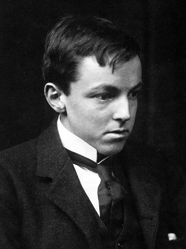
\small\textit{G. H. Hardy (1877--1947)}\\[2pt]
\tiny Public domain, via Wikimedia Commons
\end{minipage}%
\hspace{0.04\textwidth}%
\begin{minipage}[t]{0.40\textwidth}\centering
\includegraphics[width=0.70\textwidth]{images/ramanujan.jpg}\\[4pt]
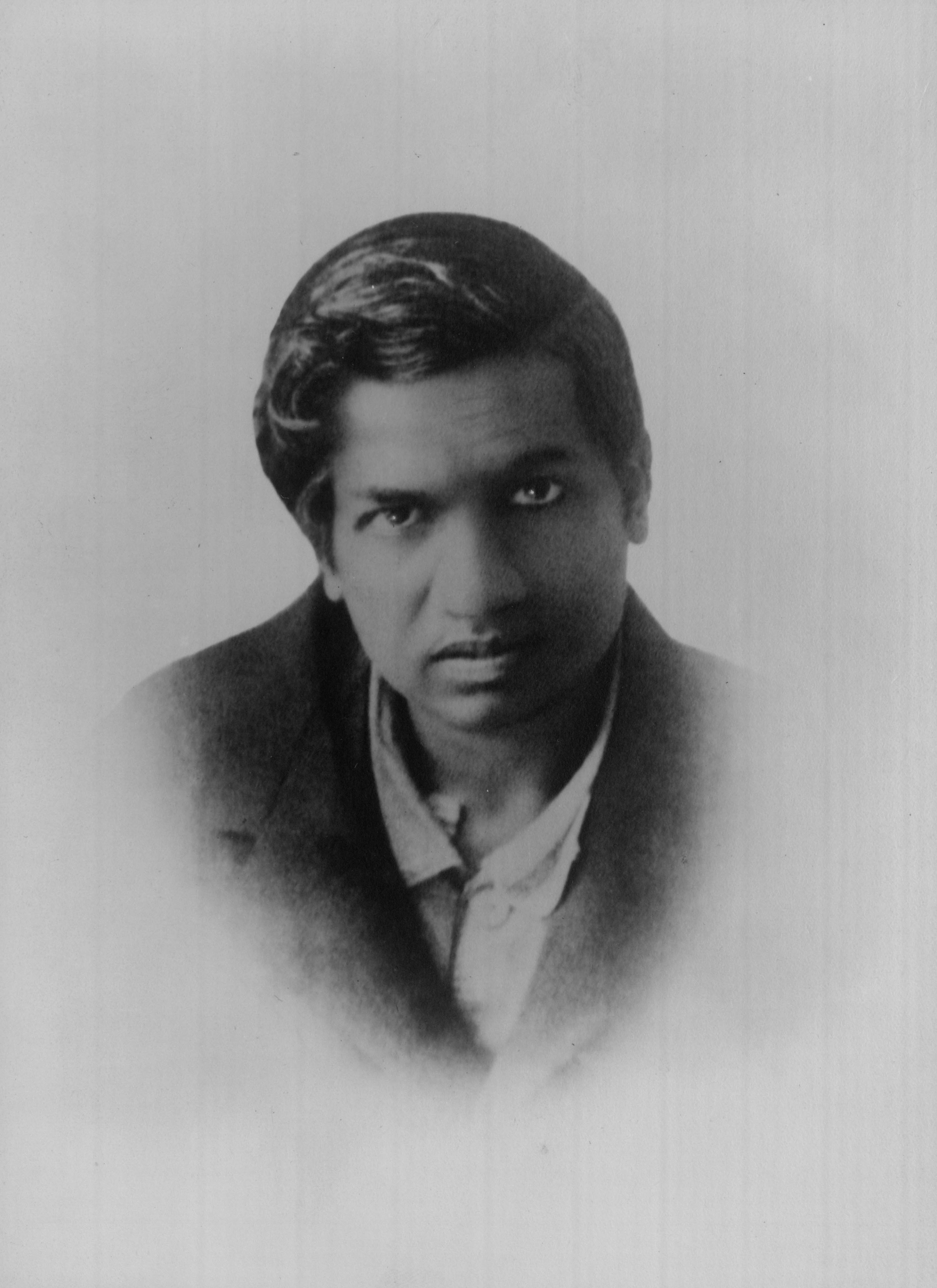
\small\textit{Srinivasa Ramanujan (1887--1920)}\\[2pt]
\tiny CC BY 4.0, Unknown author, via Wikimedia Commons
\end{minipage}
\end{center}
```
:::
::: {.content-visible when-format="html"}
<div style="display:flex; justify-content:center; gap:24px; margin:1em 0; flex-wrap:wrap;">
<div style="text-align:center; max-width:160px;">
<img src="images/hardy.jpg" style="width:120px;" alt="G. H. Hardy"><br>
<em style="font-size:0.82em;">G. H. Hardy (1877–1947)</em><br>
<span style="font-size:0.72em;">Public domain, via Wikimedia Commons</span>
</div>
<div style="text-align:center; max-width:160px;">
<img src="images/ramanujan.jpg" style="width:120px;" alt="Srinivasa Ramanujan"><br>
<em style="font-size:0.82em;">Srinivasa Ramanujan (1887–1920)</em><br>
<span style="font-size:0.72em;">CC BY 4.0, Unknown author, via Wikimedia Commons</span>
</div>
</div>
:::
In 1913, a 25-year-old clerk from Madras mailed a ten-page letter
to G. H. Hardy at Cambridge. It contained over a hundred formulas,
most with no proofs attached. Hardy nearly discarded it -- the
notation was unfamiliar and some claims seemed implausible.
What made him keep reading was that each result was stated clearly
enough to test. Hardy recognized the depth, invited the author --
Srinivasa Ramanujan -- to England, and one of the most celebrated
collaborations in mathematical history began [@kanigel1991, Ch. 4].
Every chapter of this book has followed the experimental cycle:
run code, observe patterns, form a conjecture, push it until it
breaks or holds. But a result that lives only in one notebook
changes nothing. This final chapter is about the fourth and
equally important step -- communicating what you found so that
others can read it, test it, and build on it.
::: {.content-visible when-format="pdf"}
```{=latex}
\begin{center}
\begin{minipage}[c]{0.28\textwidth}
\centering
\href{https://youtu.be/eURuh9aS3eo}{\includegraphics[width=\textwidth]{images/thumb_eURuh9aS3eo.jpg}}
\end{minipage}%
\hspace{0.02\textwidth}%
\begin{minipage}[c]{0.28\textwidth}
\small\textbf{Tibees}\\[3pt]
\small The book that Ramanujan used to teach himself mathematics\\[3pt]
\small\href{https://youtu.be/eURuh9aS3eo}{\texttt{youtu.be/eURuh9aS3eo}}
\end{minipage}%
\hspace{0.02\textwidth}%
\begin{minipage}[c]{0.36\textwidth}
\small A look at G. S. Carr's \textit{Synopsis of Pure Mathematics} --- the Victorian textbook that gave Ramanujan his mathematical vocabulary and inspired the terse, results-first style of his famous letter to Hardy.
\end{minipage}
\end{center}
```
:::
::: {.content-visible when-format="html"}
<div style="display:flex; align-items:flex-start; margin:1em 0; gap:12px; width:100%;">
<div style="flex:0 0 200px;"><a href="https://youtu.be/eURuh9aS3eo" target="_blank"><img src="https://img.youtube.com/vi/eURuh9aS3eo/0.jpg" style="width:100%;display:block;" alt="The book that Ramanujan used to teach himself mathematics"></a></div>
<div style="flex:1; font-size:0.85em;"><strong>Tibees</strong><br>The book that Ramanujan used to teach himself mathematics<br><a href="https://youtu.be/eURuh9aS3eo" target="_blank" style="font-family:monospace;">youtu.be/eURuh9aS3eo</a></div>
<div style="flex:1; font-size:0.85em;">A look at G. S. Carr's <em>Synopsis of Pure Mathematics</em> — the Victorian textbook that gave Ramanujan his mathematical vocabulary and inspired the terse, results-first style of his famous letter to Hardy.</div>
</div>
:::
## Mathematics Is a Conversation {#sec-comm-intro}
A proof published in unreadable notation is nearly useless.
A computation verified but never shared leaves mathematics
exactly where it was. Mathematics is a public activity: ideas
gain strength only when examined by more than one pair of eyes.
The style of mathematical communication has evolved over
centuries. Fermat wrote his most famous note in a book margin.
Euler described discoveries in letters across Europe. Today,
mathematics is shared in papers, posters, talks, and -- more
and more -- in code notebooks and public repositories. The
medium has changed; the purpose has not: to communicate an
idea so clearly that another person can understand it, check it,
and continue it.
Experimental mathematics adds a specific challenge. When your
result rests on computation rather than formal proof, how do you
communicate it honestly? The answer is to report the computation
itself: what was run, how far, what was found, and what the
limits of the evidence are. A reader who can reproduce your
computation can trust your conclusion, whether or not a proof
yet exists. That standard -- reproducibility -- is the same one
used in chemistry, physics, and biology. Mathematics is
discovering it too.
This chapter covers the skills needed to communicate well:
how to form and state a conjecture precisely, how to document
evidence so it is reproducible, how to structure a written report,
how to choose effective visualizations, and where to share your
work. The chapter ends with a complete sample write-up
(@sec-comm-sample) so you can see every practice in action.
## The Anatomy of a Mathematical Conjecture {#sec-comm-conjecture}
Not every observation is a conjecture. A conjecture is a specific,
testable claim that goes beyond the data already collected.
Compare these two statements:
- "The first few values of $n^2 + n + 41$ are prime."
- "For all integers $n$ with $0 \le n \le 39$, the value
$n^2 + n + 41$ is prime."
The first is a description of what you saw. The second is a
precise claim: it names the domain, the condition, and the
prediction. A conjecture must be stated precisely enough to
be proved false (see @sec-misleads-fail for examples of
striking patterns that did fail).
A well-formed mathematical conjecture has five parts:
1. **The observation**: the numerical pattern that started the
question.
2. **The data**: a table or list showing the pattern concretely.
3. **The precise statement**: a single sentence with explicit
quantifiers ("for all $n$", "there exists $p$") that turns
the pattern into a testable claim.
4. **The tested range**: how far the computation has verified
the claim.
5. **The open question**: what would need to be proved for the
pattern to hold always, and whether that is currently known.
Here is Goldbach's conjecture (@sec-primes-goldbach) written out
in this structure as a model:
- **Observation**: every even number we checked can be written
as a sum of two primes.
- **Data**: $4 = 2+2$, $6 = 3+3$, $8 = 3+5$, $10 = 3+7$,
$100 = 3+97$.
- **Precise statement**: every even integer $n \ge 4$ is the
sum of two prime numbers.
- **Tested range**: verified for all even $n$ up to
$4 \times 10^{18}$ as of 2014 [@oliveira2014].
- **Open question**: no proof exists for all $n$. It is one of
the oldest open problems in number theory.
Notice that the open question is as valuable as the precise
statement. It tells readers where the frontier is and invites
them to push forward. Leaving it out sends the message that the
problem is solved -- which is the opposite of what experimental
mathematics is about.
## Documenting Computational Evidence {#sec-comm-evidence}
Good computational evidence is reproducible. If you write in
your report that "the conjecture holds for all even $n$ up to
10,000," a reader must be able to run your code and obtain the
same result. Four practices make evidence reproducible:
- **Name your bound** with a variable (`UPPER = 10_000`) rather
than burying the number in a loop condition. A reader can then
change the bound and rerun immediately.
- **Report failures explicitly**: a loop that finds no failures
is convincing; a loop that silently skips edge cases is not.
Print the failing cases when they exist.
- **Include a success message that states the range**, not just
an absence of error. "No failures found" is weaker than
"Goldbach verified for all even n from 4 to 10,000."
- **Fix random seeds** when your code uses randomness, so
results are reproducible. The `random.seed` function, used
in the Ulam spiral code at @sec-primes-ulam, is the standard
way to do this in Python.
The code below demonstrates these practices on the Goldbach
conjecture. The `isprime` function was introduced at
@sec-primes-what.
```{python}
from sympy import isprime

def is_goldbach(n):
    # Returns True if n is a sum of two primes.
    for p in range(2, n // 2 + 1):
        if isprime(p) and isprime(n - p):
            return True
    return False

UPPER = 10_000  # name the tested range explicitly
failures = [
    n for n in range(4, UPPER + 1, 2)
    if not is_goldbach(n)
]

if failures:
    print(
        f"Conjecture FAILS at: {failures[:5]}"
    )
else:
    print(
        "Goldbach verified for all even n"
        f" from 4 to {UPPER:,}."
    )
```
The output names the range. A reader who sees this knows
exactly what was and was not checked.
One discipline often overlooked: always test edge cases.
Does your code handle the smallest possible input (here $n = 4$)?
Does it handle prime inputs correctly? Edge cases are where
patterns most often break first -- and where the most surprising
mathematics hides.
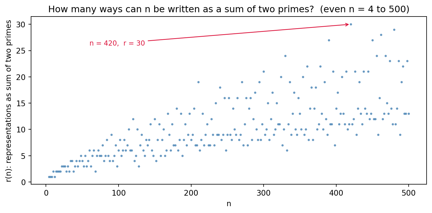
The verification above answers a yes/no question. But how many
ways can each even $n$ be expressed as a sum of two primes?
Define $r(n)$ as the count of pairs $(p, q)$ with $p \le q$ and
$p + q = n$, both prime. Plotting $r(n)$ reveals that the answer
is never zero -- and that the count has its own hidden structure.
### Research Example: Is Every Even Number a Sum of Two Primes in the Same Number of Ways? {.unnumbered .unlisted}
Goldbach's conjecture says every even $n \ge 4$ can be written as a sum of two primes
at least once, but it says nothing about how many ways. Does the count $r(n)$ grow
steadily, stay flat, or vary wildly from one even number to the next?
```{python}
#| label: fig-comm-goldbach-reps
#| fig-cap: "Goldbach representation count r(n) for even n from 4 to 500. Each dot is one even number; its height counts the ordered pairs (p, q) with p ≤ q, p + q = n, and both p, q prime. Highly composite numbers consistently reach higher peaks."
from sympy import isprime
import matplotlib.pyplot as plt

def goldbach_reps(n):
    return sum(
        1 for p in range(2, n // 2 + 1)
        if isprime(p) and isprime(n - p)
    )

evens_gr = list(range(4, 502, 2))
reps_gr  = [goldbach_reps(n) for n in evens_gr]

peak_val = max(reps_gr)
peak_n   = evens_gr[reps_gr.index(peak_val)]

fig, ax = plt.subplots(figsize=(8, 4))
ax.scatter(evens_gr, reps_gr, s=4,
           color='steelblue', alpha=0.7)
ax.annotate(
    f'n = {peak_n},  r = {peak_val}',
    xy=(peak_n, peak_val),
    xytext=(60, peak_val - 4),
    arrowprops=dict(arrowstyle='->',
                    color='crimson'),
    color='crimson', fontsize=9)
ax.set_xlabel('n')
ax.set_ylabel('r(n): representations as sum of two primes')
ax.set_title(
    'How many ways can n be written as'
    ' a sum of two primes?  (even n = 4 to 500)')
plt.tight_layout()
plt.show()
```
Not only is $r(n)$ never zero (no counterexample to Goldbach here), it actually tends to
grow — numbers with many divisors offer many ways to split into two primes. The scatter
is wide but the floor stays safely above zero, making the conjecture look very sturdy
over this range.
Chapter 14 established the most important caution: computational
evidence is not proof (@sec-misleads-danger). Patterns that hold
for thousands of cases can fail. Report your evidence, label it
as evidence, and never write "holds for all $n$" when you mean
"holds for all tested $n$ up to 10,000."
## Writing Up a Research Report {#sec-comm-report}
A mathematical research report has three main sections [@martin2011, §1.3].
**Section 1: Statement of the Problem.** State the problem in
your own words. Why is it interesting? What is already known?
What question are you asking? This section should be readable
by someone who has not seen the problem before. It is also the
place to cite prior work: if someone else studied the same
problem, say so and say what you found that they did not.
**Section 2: Description of the Solution Procedure.** Describe
the mathematics and code you used. Name algorithms ("sieve of
Eratosthenes," "fast modular exponentiation") rather than
describing the code in informal terms. Show the key formulas.
Include the central computation -- either as pseudo-code or
as the actual Python code block. Do not include every helper
function; show the ideas.
**Section 3: Results and Conclusions.** Report what you found:
tables, figures, and conjectures. State precisely what your
evidence shows. If you made a conjecture, say how far you tested
it. Describe difficulties you encountered and what you could not
resolve. Suggest ways to extend the work. Every table and figure
should have a caption; every captioned figure should be referred
to by name in the text.
A few style points that separate a professional report from a
homework solution:
- Write every figure caption as a complete sentence that makes
sense without the surrounding text.
- Number every equation or formula you refer to later.
Quarto does this automatically when you add `\label{eq:name}`
and use `\eqref{eq:name}` in the text.
- Use variable names in prose that match your code. If your
code uses `UPPER` as the search bound, write "UPPER = 10,000"
in the text, not "ten thousand."
- Code is graded on both performance (does it produce correct
results?) and style (is it readable?). Descriptive variable
names, clearly labeled output, and logical function organization
all contribute to style.
In Quarto, mathematical notation is automatic. Inline formulas
use `$...$` (for example, `$n^2 + n + 41$` renders as
$n^2 + n + 41$). Displayed equations use `$$...$$`. No separate
LaTeX installation is needed for the HTML output of this book.
## Effective Mathematical Visualizations {#sec-comm-viz}
A picture can reveal structure that no table can.
In 1983, mathematicians David Hoffman and William Meeks III were
trying to understand a new kind of minimal surface -- a
mathematical soap film of infinite extent. The equations gave
them almost no intuition. When they plotted the surface on a
computer, the geometry became visible. "The surface couldn't be
understood until we could see it," Hoffman said. "Once we saw
it on the screen, we could go back to the proof." [@borwein2009crucible, Ch. 11]
This is visualization as a tool for discovery, not decoration.
And it applies directly to the computations in this book.
Here are five rules for effective mathematical plots.
1. **Label every axis.** If the reader cannot tell what the
axes represent, the plot communicates nothing.
2. **Write a title** that states the claim or subject, not just
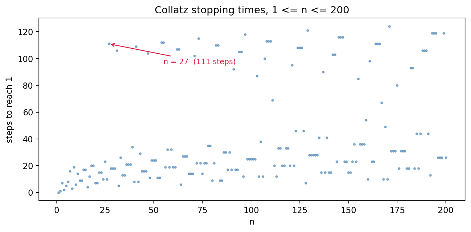
a vague topic. "Collatz stopping times for $1 \le n \le 200$"
beats "Stopping times."
3. **Annotate notable points.** If one value stands out, point
to it. Do not leave readers wondering why n = 27 produces a
spike in the Collatz scatter plot.
4. **Use markers or line styles that survive grayscale printing.**
A PDF printed in black and white loses color. Combine color
with different marker shapes or dashed vs. solid lines.
5. **Write a caption** as a complete sentence describing what
the reader should notice.
The code below applies all five rules to the Collatz stopping
times. The function `collatz_stopping` was introduced at
@sec-collatz-loop; it is redefined here because each Quarto
chapter runs in its own Python kernel.
```{python}
import matplotlib.pyplot as plt

# Redefined here; first introduced at @sec-collatz-loop.
def collatz_stopping(n):
    steps = 0
    while n != 1:
        n = n // 2 if n % 2 == 0 else 3 * n + 1
        steps += 1
    return steps

ns = list(range(1, 201))
times = [collatz_stopping(n) for n in ns]

fig, ax = plt.subplots(figsize=(8, 4))
ax.scatter(
    ns, times, s=5, color='steelblue',
    alpha=0.6)
ax.set_xlabel('n')
ax.set_ylabel('steps to reach 1')
ax.set_title(
    'Collatz stopping times, 1 <= n <= 200')
ax.annotate(
    'n = 27  (111 steps)',
    xy=(27, 111),
    xytext=(55, 96),
    arrowprops=dict(
        arrowstyle='->',
        color='crimson'),
    color='crimson',
    fontsize=9)
plt.tight_layout()
plt.show()
```
Both axes are labeled, the title describes the content, and
n = 27 is explicitly identified. A reader encountering this
figure for the first time knows exactly what they are looking at
and why n = 27 is worth noticing.
## Where to Share Your Work {#sec-comm-share}
Research that stays in a notebook changes nothing. Here are
five paths for sharing computational mathematical discoveries
at the high school and undergraduate level, roughly in order
of effort required.
**The OEIS.** The On-Line Encyclopedia of Integer Sequences
(@sec-oeis-database) accepts contributions from anyone. If you
discover a new sequence or compute new terms for an existing one,
you can submit directly at oeis.org. An OEIS entry requires the
first several terms, a precise definition, and sample code.
This is often the fastest path to a permanent, citable record.
**A public notebook.** A Quarto document or Jupyter notebook
published on GitHub is immediately accessible and reproducible.
It is not peer-reviewed, but it is shareable, linkable, and
can be assigned a permanent DOI through Zenodo. Many
mathematicians share preliminary results this way before formal
submission.
**Undergraduate posters and talks.** Regional Mathematical
Association of America (MAA) section meetings hold undergraduate
poster sessions and contributed talks every spring. The format
is short -- posters run for about an hour; talks are 12 to 15
minutes -- but the audience is knowledgeable and welcoming.
Preparing a poster forces you to distill your work to its
essential claim and evidence. Many students present at regional
conferences before their work is publication-ready [@martin2011, §1.3.2].
**Undergraduate research journals.** Several peer-reviewed
journals publish original undergraduate mathematics: *Involve*,
the *Pi Mu Epsilon Journal*, and *SIAM Undergraduate Research
Online* (SIURO). These are refereed and take several months.
The standard is the same as for professional journals: clarity,
originality, and either a proof or compelling computational
evidence presented reproducibly.
**arXiv preprints.** The arXiv (arxiv.org) hosts preprints
before formal publication. No university affiliation is
required, though first-time submitters need an endorser.
A preprint is not peer-reviewed but establishes priority,
and it is widely read -- many mathematicians check arXiv daily.
Whatever path you choose: start sharing sooner than you feel
ready. The feedback will improve your work faster than additional
computation will.
## A Sample Write-Up: Stopping Time Records {#sec-comm-sample}
The following pages present a complete mini research report on
Collatz stopping-time records. Read it as a template: notice the
three-section structure, the precision of the conjecture, the
way the code is presented and discussed, and how the figures and
tables are described. After you read it, try writing one of your
own on a topic from any earlier chapter.
---
### The Problem
The Collatz stopping time of a positive integer $n$ is the number
of steps the Collatz rule needs to reach 1 (see @sec-collatz-stopping).
For $n = 3$, for example, the path
$3 \to 10 \to 5 \to 16 \to 8 \to 4 \to 2 \to 1$ takes 7 steps.
Some numbers have stopping times far longer than their neighbors.
We call $n$ a **stopping-time record-setter** if its stopping time
is strictly greater than the stopping time of every smaller
positive integer. For instance, $n = 3$ is a record-setter because
no number from 1 to 2 has a stopping time greater than 7.
**Research question.** Which integers are stopping-time record-setters,
and how rapidly do the record stopping times grow?
This question is accessible with the tools developed in Chapter 4,
touches the unsolved Collatz conjecture, and produces a result we
can actually prove -- a rare combination.
### Solution Procedure
We define `collatz_stopping(n)` as in @sec-collatz-loop, then scan
$n$ from 1 to an upper bound $N$, tracking the running maximum
stopping time. Every time a new maximum is reached, we record the
pair $(n, t)$.
```{python}
# collatz_stopping: first introduced at @sec-collatz-loop.
# Redefined here because each chapter runs in its own kernel.

def collatz_stopping(n):
    steps = 0
    while n != 1:
        n = n // 2 if n % 2 == 0 else 3 * n + 1
        steps += 1
    return steps

N = 100_000
records = []
max_steps = -1          # start below 0 to capture n=1

for n in range(1, N + 1):
    s = collatz_stopping(n)
    if s > max_steps:
        max_steps = s
        records.append((n, s))

print(f"Record-setters found up to N={N:,}: "
      f"{len(records)}")
print(f"Largest record: n={records[-1][0]}, "
      f"t={records[-1][1]}")
```
The table below lists the first 20 record-setters. The third
column shows the ratio $t / \log_2 n$, where $t$ is the stopping
time. (`math.log` with two arguments was introduced at
@sec-cfrac-gauss-kuzmin.)
```{python}
import math

header = (
    f"{'n':>9}  {'t':>5}  {'t/log2(n)':>10}"
)
print(header)
print("-" * 30)
for n, t in records[:20]:
    if n <= 1:
        row = f"{n:9d}  {t:5d}  {'---':>10}"
    else:
        ratio = t / math.log(n, 2)
        row = (
            f"{n:9d}  {t:5d}  {ratio:10.2f}"
        )
    print(row)
```
### Results and Conclusions
Three patterns emerge from the table.
**Pattern 1: consecutive pairs near $2k$.** Every time an odd
record-setter $n$ appears, the number $2n$ appears immediately
after with stopping time one higher. For example: $(27, 111)$
is followed by $(54, 112)$; $(9, 19)$ by $(18, 20)$. This is not
a coincidence -- it follows from the Collatz rule: $2n \to n$ in
exactly one step, so $t(2n) = t(n) + 1$ always.
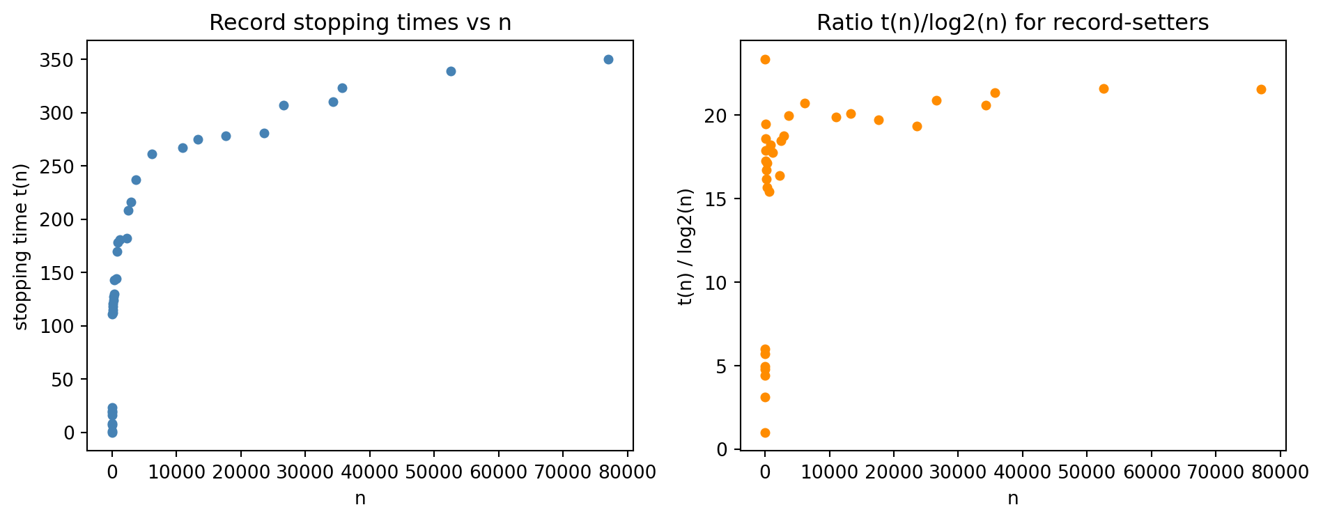
**Pattern 2: the ratio $t / \log_2 n$ does not grow.** The
right column of the table oscillates without a clear upward
trend, suggesting that the stopping times of record-setters
grow at most logarithmically in $n$.
We state this as a formal conjecture:
> **Conjecture.** There exists a constant $C$ such that for
> every stopping-time record-setter $n$, the stopping time
> $t(n)$ satisfies $t(n) \le C \cdot \log_2 n$.
**Pattern 3: ratio of consecutive record-setters is at most 2.**
Looking at the $n$ column, the ratio between any record-setter
and the one before it never exceeds 2. For example:
$27/25 = 1.08$, $54/27 = 2$, $73/54 \approx 1.35$.
This pattern has a proof.
**Proved fact.** If $n$ is a stopping-time record-setter, the
next record-setter $m$ satisfies $m \le 2n$ (ratio at most 2).
*Proof.* Because $2n$ is even, the Collatz rule maps $2n \to n$
in one step, so $t(2n) = t(n) + 1 > t(n)$. This means $2n$ is
a candidate for the next record. The next record-setter $m$ is
the smallest integer greater than $n$ with $t(m) > t(n)$. Since
$2n$ is one such integer, $m \le 2n$, giving the ratio
$m/n \le 2$. $\square$
The visualization below confirms both the logarithmic growth
and the bounded ratio.
```{python}
import matplotlib.pyplot as plt

rec_n = [r[0] for r in records]
rec_t = [r[1] for r in records]

# Ratio t/log2(n) for n >= 2 (log(1) = 0)
ratio_data = [
    (n, t / math.log(n, 2))
    for n, t in records
    if n >= 2
]
ratio_n = [p[0] for p in ratio_data]
ratio_r = [p[1] for p in ratio_data]

fig, axes = plt.subplots(1, 2, figsize=(10, 4))

ax = axes[0]
ax.scatter(rec_n, rec_t, s=18,
           color='steelblue')
ax.set_xlabel('n')
ax.set_ylabel('stopping time t(n)')
ax.set_title('Record stopping times vs n')

ax = axes[1]
ax.scatter(ratio_n, ratio_r,
           s=18, color='darkorange')
ax.set_xlabel('n')
ax.set_ylabel('t(n) / log2(n)')
ax.set_title(
    'Ratio t(n)/log2(n) for record-setters')

plt.tight_layout()
plt.show()
```
The left panel shows that stopping times grow, but slowly.
The right panel shows the ratio oscillating without a clear
upward trend up to $N = 100{,}000$. Whether the ratio remains
bounded as $N \to \infty$ is an open question connected to
the unsolved Collatz conjecture itself.
**Open question.** Are there infinitely many record-setters
that are NOT equal to twice the previous record-setter? The data
above suggests yes -- numbers like 27 beat the previous record
by a large margin without coming from $2 \times \text{(previous)}$.
But no proof is known.
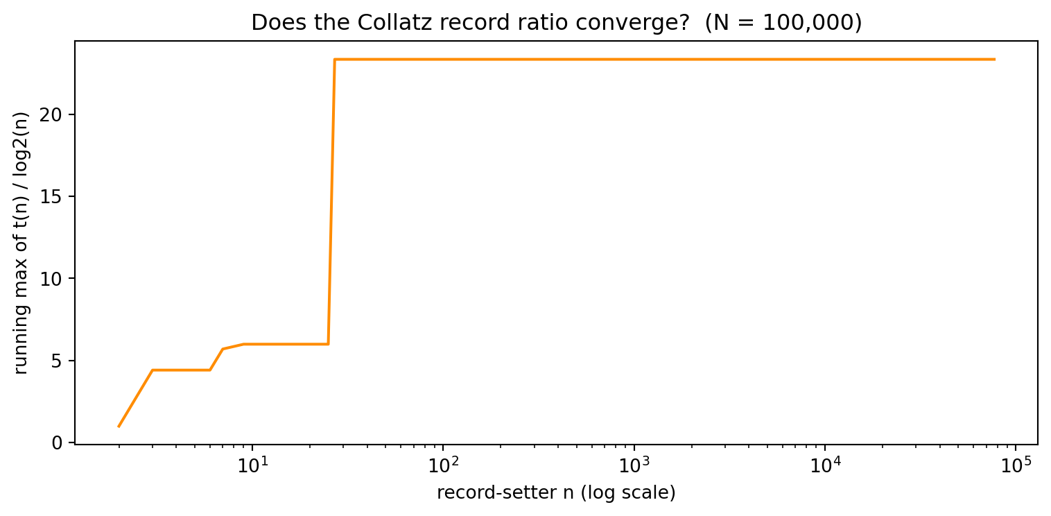
The running maximum of the ratio $t(n)/\log_2 n$ across all
record-setters up to $N = 100{,}000$ makes this visible directly.
If the conjecture holds, the curve should plateau.
```{python}
#| label: fig-comm-ratio-max
#| fig-cap: "Running maximum of the ratio t(n)/log₂(n) for Collatz stopping-time record-setters up to N = 100,000. Each step up marks a new record-setter that beats every predecessor's ratio. If the ratio is truly bounded, the curve converges to a finite ceiling."
# uses: records (Collatz stopping-time record-setters computed above)
import math
import matplotlib.pyplot as plt

ratio_pairs_rm = [
    (n, t / math.log(n, 2))
    for n, t in records
    if n >= 2
]
cur_max_rm = 0.0
running_max_rm = []
for n_rm, r_rm in ratio_pairs_rm:
    if r_rm > cur_max_rm:
        cur_max_rm = r_rm
    running_max_rm.append((n_rm, cur_max_rm))

rm_n_vals = [p[0] for p in running_max_rm]
rm_r_vals = [p[1] for p in running_max_rm]

fig, ax = plt.subplots(figsize=(8, 4))
ax.semilogx(rm_n_vals, rm_r_vals,
            color='darkorange', linewidth=1.5)
ax.set_xlabel('record-setter n (log scale)')
ax.set_ylabel('running max of t(n) / log2(n)')
ax.set_title(
    'Does the Collatz record ratio converge?'
    '  (N = 100,000)')
plt.tight_layout()
plt.show()
```
---
That ends the sample report. Notice what it contains: a
motivated problem statement, code with a named bound, a table,
two visualizations with labeled axes, a formal conjecture, and
a proved sub-result. Not every research report will include a
proof -- but every report should state clearly what is known
and what is not.
## Summary: The Experimental Mathematics Workflow {#sec-comm-workflow}
Thirteen chapters of computation have followed a single cycle.
| Step | What it means | Where in this book |
|------|---------------|--------------------|
| Explore | Run code, generate data, notice patterns | Chapters 1--14 |
| Conjecture | State a precise, testable claim | Throughout |
| Test | Extend the range; try to break the pattern | Chapter 14 |
| Communicate | Report the result so others can build on it | This chapter |
The cycle is not linear. A visualization prepared for
communication often reveals a new pattern. A new pattern
produces a sharper conjecture. A sharper conjecture exposes
a failure case that no one expected. The cycle repeats, and
each loop produces more understanding.
The computations in this book were chosen not because they are
solved, but because they are accessible and open. Every
"Further Research Topics" section ends with directions that
genuine mathematicians have not fully explored. When a student
stares at the Ulam spiral and notices a diagonal stripe not
mentioned in any textbook -- or finds a Pisano period that
seems to be prime for reasons they cannot explain -- or
discovers that the ratio of Collatz records appears bounded
by a constant that looks familiar -- that moment of
"I wonder if..." is the beginning of mathematics.
The computers available to you today are more powerful than
anything Euler, Gauss, or Ramanujan ever had access to.
The tools -- Python, SymPy, mpmath, matplotlib -- are free,
documented, and run on any laptop. The open problems are not
locked behind graduate degrees or expensive software. They
sit in the data, waiting for someone to look carefully enough.
Look carefully.
## Further Research Topics {#sec-comm-research}
1. Choose any result from Chapters 1 through 13 that surprised
you. Write a one-page summary in the three-section format
from @sec-comm-report: problem statement, solution procedure,
results and conclusions. The goal is practice with the format,
not new discoveries.
*(Problem proposed by Claude Code.)*
2. Take any scatter plot from this book and redraw it following
all five visualization rules from @sec-comm-viz: labeled axes,
descriptive title, annotated outlier, print-safe markers,
and a complete caption. In one paragraph, explain what the
improved plot communicates that the original did not.
*(Problem proposed by Claude Code.)*
3. Verify the ratio $\le 2$ result computationally for all
Collatz stopping-time record-setters up to $N = 1{,}000{,}000$.
Do any ratios come close to 2 for large $n$? Report your
findings in the three-section format from @sec-comm-report.
*(Problem proposed by Claude Code.)*
4. Find all Collatz stopping-time record-setters up to $N = 500$.
Look at each one in base 3 (hint: `int(n)` converted digit
by digit using `n % 3` and `n // 3` in a loop). Make a
conjecture about which base-3 digit patterns appear most
often among record-setters.
*(Problem proposed by Claude Code.)*
5. The sequence of Collatz stopping-time record-setters begins
1, 2, 3, 6, 7, 9, 18, 25, 27, ... Search the OEIS
(@sec-oeis-database) for these terms. Does the OEIS entry
match your computed data? What additional information or
references does it provide?
*(Problem proposed by Claude Code.)*
6. Define the "shortcut stopping time" of $n$ as the number of
Collatz steps until the sequence first reaches a value
smaller than $n$ (rather than reaching 1). Find the
record-setters for the shortcut stopping time up to $N = 10{,}000$
and compare them to the standard record-setters from this
chapter. Are they the same numbers?
*(Problem proposed by Claude Code.)*
7. Extend the Goldbach verification from @sec-comm-evidence to
$\text{UPPER} = 1{,}000{,}000$. Time the computation using
Python's `time` module. Estimate how long the same algorithm
would need to verify Goldbach up to $10^9$. What change to
the code would give the largest speedup?
*(Problem proposed by Claude Code.)*
8. Prove the following extension of the ratio theorem from
@sec-comm-sample: if $n$ is a stopping-time record-setter
and $n$ is odd, then $n$ is not equal to $2k$ for any other
record-setter $k$. (Hint: use the fact that $2k \to k$ in
one step and $n$ odd means $n \ne 2k$ for any integer $k$.)
*(Problem proposed by Claude Code.)*
9. Write a complete research report (three sections, 2--4 pages,
at least one figure and one formal conjecture) on one of the
"Further Research Topics" from any earlier chapter. Include
at least one computation not already done in the book.
*(Problem proposed by Claude Code.)*
10. Compare the growth of Collatz stopping-time record-setters
to the growth of prime record-gaps from @sec-primes-gaps:
integers $n$ where the gap to the next prime exceeds all
previous prime gaps. Do both sequences grow roughly like
$O(\log n)$? Write a report with a visualization overlaying
both sequences on the same plot.
*(Problem proposed by Claude Code.)*
11. The weak Goldbach conjecture -- every odd integer $\ge 7$ is
the sum of three primes -- was proved by Harald Helfgott in
2013 after centuries as an open problem. Verify it
computationally for all odd $n$ from 7 to 100,000. Write a
report explaining the result to a high school audience, with
your verification code and a discussion of how many
representations each odd $n$ typically has [@helfgott2013].
*(Problem proposed by Claude Code.)*
12. Create a poster (one printed page or one slide) summarizing
one chapter of this book for an audience of students who have
not read it. Apply the principles from @sec-comm-report: clear
layout, figures in place of text where possible, and a design
that is self-explanatory without an oral companion. Present
the poster to a class and gather feedback using the five
visualization rules as your rubric.
*(Problem proposed by Claude Code.)*
13. Research the history and proof of the Four Color Theorem.
When was it first conjectured? When was it proved, and what
role did computers play? Write a 2--3 page report explaining
the key ideas to a high school reader -- no technical graph
theory required. Include a Python visualization of a small
planar map colored with four colors [@borwein2009crucible, Ch. 11].
*(Adapted from @borwein2009crucible.)*
14. Find a new integer sequence arising from any computation in
this book that is not already in the OEIS (check at oeis.org
before spending time on this). Submit it. Document the
submission process: what information is required, how the
sequence is formatted, and how long approval takes. Report
the outcome to your class.
*(Problem proposed by Claude Code.)*
15. Using the mpmath library (@sec-constants-mpmath), compute the
ratio $t(n) / \log_2 n$ for the 100 largest known Collatz
stopping-time record-setters to 30 decimal places. Does the
ratio appear to converge to a recognizable constant -- perhaps
a multiple of $\log 2$, or $\pi$, or the Feigenbaum constant
from @sec-logistic-feigenbaum? Use the PSLQ algorithm ideas
from Chapter 9 to search for an integer relation.
*(Problem proposed by Claude Code.)*
16. The Green--Tao theorem (2004) guarantees that prime numbers
contain arithmetic progressions of every finite length [@green2008].
Write a Python program that finds all arithmetic progressions
of primes with at least five terms whose first term is at most
1,000. For each progression, report the first prime $p$, the
common difference $d$, and the length. Which five-term progression
has the largest common difference? Plot the count of such
progressions as the upper bound on $p$ increases from 100 to
1,000. State a conjecture about how this count grows. Write a
complete three-section report following @sec-comm-report,
including a visualization that places the longest progressions
on a number line so a reader can see them at a glance.
*(Problem proposed by Claude Code.)*
17. A **referee report** is what a peer reviewer submits when a
journal editor asks them to evaluate a submitted paper.
Find a short, publicly available "proof attempt" of a famous
open conjecture -- searches on arXiv for "Collatz conjecture
proof" or "Goldbach conjecture elementary proof" will surface
examples. Read it carefully. Then write a one-to-two page
referee report that: (a) states the paper's central claim in
your own words, (b) identifies the first step where the
argument is incomplete or breaks down, and (c) proposes a
specific computational check that would either support or
refute that step. This exercise trains the skill of reading
mathematics critically -- which is as important as writing it,
and far rarer. The report should be written for an audience
of fellow students, not for the original authors.
*(Problem proposed by Claude Code.)*
18. Design a complete research project from scratch. Choose any
mathematical operation or sequence not already studied in this
book. Generate the first 100 terms in Python, search the OEIS
(@sec-oeis-database) for matches, state at least one testable
conjecture, and verify it computationally to a bound you choose
and justify. Write a full three-section report (@sec-comm-report)
with at least two figures with proper captions. If the sequence
is genuinely new -- meaning it appears nowhere in the OEIS --
prepare a draft OEIS submission following the format from topic 14.
Document every step of the experimental cycle from
@sec-comm-workflow in a final paragraph: what surprised you,
what failed, and what remains open. This is the capstone of the
book: the complete arc from a half-formed curiosity to a
communicable result.
*(Problem proposed by Claude Code.)*