# Prime Numbers: The Atoms of Arithmetic {#sec-primes}
Every integer greater than 1 can be broken into smaller pieces --- except
for the primes. A prime number has no divisors other than 1 and itself,
which makes it irreducible, a genuine atom of the integers. The ancient
Greeks knew this, and Euclid proved around 300 BCE that the supply of
primes is inexhaustible. Yet two thousand years later, some of the
simplest questions about primes remain wide open: Are there infinitely
many twin primes? Can every even number be written as a sum of two primes?
No one knows.
What computation *can* do is explore. In this chapter we will sieve for
primes, count them, measure the gaps between them, and visualize their
hidden structure. Along the way a striking fact will emerge: primes, which
seem random, are surprisingly orderly.
## What Is a Prime? {#sec-primes-what}
```{python}
#| echo: false
from pathlib import Path; import urllib.request
_d = Path('images'); _d.mkdir(exist_ok=True)
_p = _d / 'euclid.jpg'
if not _p.exists():
try: urllib.request.urlretrieve('https://upload.wikimedia.org/wikipedia/commons/3/30/Euklid-von-Alexandria_1.jpg', _p)
except Exception: pass
```
::: {.content-visible when-format="pdf"}
```{=latex}
\begin{center}
\begin{minipage}[c]{0.22\textwidth}
\includegraphics[width=\textwidth]{images/euclid.jpg}
\end{minipage}%
\hspace{0.03\textwidth}%
\begin{minipage}[c]{0.35\textwidth}
\small\textit{Euclid of Alexandria (c.~300 BCE)}\\[2pt]
\tiny Wellcome Collection (CC BY 4.0)
\end{minipage}
\end{center}
```
:::
::: {.content-visible when-format="html"}
<div style="display:flex; align-items:center; margin:1em 0; gap:12px;">
<img src="images/euclid.jpg" style="width:100px; flex-shrink:0;" alt="Euclid of Alexandria">
<div style="font-size:0.82em;"><em>Euclid of Alexandria (c. 300 BCE)</em><br><span style="font-size:0.85em;">Wellcome Collection (CC BY 4.0)</span></div>
</div>
:::
A positive integer $n > 1$ is **prime** if its only positive divisors are
$1$ and $n$. Otherwise it is **composite**. The integer $1$ is neither
prime nor composite --- it is its own special case, the one number that
divides everything without contributing to any factorization.
The first few primes are $2, 3, 5, 7, 11, 13, 17, 19, 23, 29, \ldots$
Note that $2$ is the only even prime: every other even number is divisible
by $2$.
The **Fundamental Theorem of Arithmetic** guarantees that every integer
$n \geq 2$ can be written as a product of primes in exactly one way (up
to reordering). For example:
$$360 = 2^3 \cdot 3^2 \cdot 5$$
SymPy's `isprime` and `factorint` make it easy to explore factorizations.
```{python}
from sympy import isprime, factorint, nextprime

for n in [2, 17, 18, 360, 1001]:
    if isprime(n):
        print(f"{n} is prime")
    else:
        print(f"{n} = {factorint(n)}")
```
`factorint` returns a dictionary whose keys are prime factors and whose
values are exponents. So `{2: 3, 3: 2, 5: 1}` means $2^3 \cdot 3^2 \cdot
5^1 = 360$.
We can collect the first 25 primes using `nextprime`, which returns the
smallest prime larger than its argument.
```{python}
import pprint
primes_25 = []
p = 2
while len(primes_25) < 25:
    primes_25.append(p)
    p = nextprime(p)
# width=60 wraps long output to fit the printed page
pprint.pprint(primes_25, width=60, compact=True)
```
**Why are there infinitely many primes?** Euclid's argument is one of the
most elegant in all of mathematics. Suppose we had a complete list
$p_1, p_2, \ldots, p_k$ of *all* primes. Form the number
$N = p_1 \cdot p_2 \cdots p_k + 1$. Then $N$ is not divisible by any
$p_i$ (it always leaves remainder $1$), so either $N$ itself is prime or
it has a prime factor not on our list. Either way, the list was incomplete.
Since any finite list fails, the primes are infinite.
## Finding Primes: The Sieve of Eratosthenes {#sec-primes-sieve}
```{python}
#| echo: false
from pathlib import Path; import urllib.request
_d = Path('images'); _d.mkdir(exist_ok=True)
_p = _d / 'eratosthenes.jpg'
if not _p.exists():
try: urllib.request.urlretrieve('https://upload.wikimedia.org/wikipedia/commons/b/bc/Eratosthenes.jpg', _p)
except Exception: pass
```
::: {.content-visible when-format="pdf"}
```{=latex}
\begin{center}
\begin{minipage}[c]{0.22\textwidth}
\includegraphics[width=\textwidth]{images/eratosthenes.jpg}
\end{minipage}%
\hspace{0.03\textwidth}%
\begin{minipage}[c]{0.35\textwidth}
\small\textit{Eratosthenes of Cyrene (c.~276--194 BCE)}\\[2pt]
\tiny Public domain
\end{minipage}
\end{center}
```
:::
::: {.content-visible when-format="html"}
<div style="display:flex; align-items:center; margin:1em 0; gap:12px;">
<img src="images/eratosthenes.jpg" style="width:100px; flex-shrink:0;" alt="Eratosthenes of Cyrene">
<div style="font-size:0.82em;"><em>Eratosthenes of Cyrene (c. 276–194 BCE)</em><br><span style="font-size:0.85em;">Public domain</span></div>
</div>
:::
Calling `isprime` one number at a time is fine for a few values, but slow
if you need *all* primes up to a million. The **Sieve of Eratosthenes**,
invented around 240 BCE, is dramatically faster: start with a list of all
integers from $2$ to some limit, then repeatedly cross out all multiples
of each prime you find. In other words, it does not find prime numbers. It knocks out what is *not* prime number repeatedly until all are gone, so that the survivors can be called prime. There is something brutal and satisfying about this 2260-year-old algorithm.
But how many numbers and their multiples do we knock down? Suppose we are looking all prime number under $1000$, we would start knocking out all multiples of $2$, of $3$, ... up to? Certainly we don't have to go as high as $999$ because there is no number that one could multiply to $999$ to get $1000$. How about 500? Sure, $500 \cdot 2 = 1000$. But $500$ was already knocked out when the multiples of $2$ were worked on. The same goes for $250$.
```{python}
def factor_pairs(n):
    pairs = []
    for left in range(1, n + 1):
        if n % left == 0:
            right = n // left
            print(f"{n} = {left} * {right}")
            pairs.append((left, right))
    return pairs

n = 1000
pairs = factor_pairs(n)
```
The key insight is that if $n$ is composite, it must have a prime factor
$p \leq \sqrt{n}$. So we only need to sieve with primes up to
$\sqrt{\text{limit}}$, after which every surviving number is prime.
```{python}
def sieve(limit):
    """Return list of all primes up to limit."""
    is_prime = [True] * (limit + 1)
    is_prime[0] = is_prime[1] = False
    i = 2
    while i * i <= limit:   # only need to sieve up to sqrt(limit)
        if is_prime[i]:
            for j in range(i * i, limit + 1, i):  # i² already cleared
                is_prime[j] = False
        i += 1
    return [k for k in range(limit + 1) if is_prime[k]]

print(sieve(50))
```
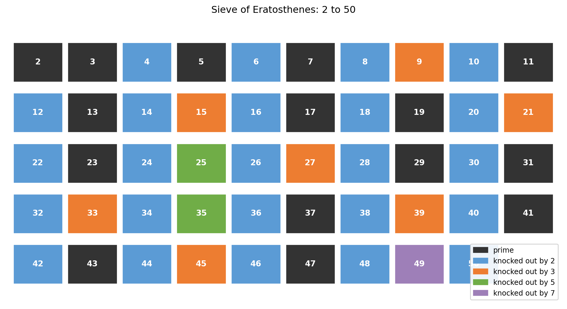
### Research Example: Who Gets Knocked Out First? {.unnumbered .unlisted}
Which prime claims the most territory in the sieve — and how much do the later primes even contribute? Color every composite by the first prime that eliminates it and the answer jumps off the page.
```{python}
# uses: sieve()
import matplotlib.pyplot as plt
import matplotlib.patches as mpatches

nums = list(range(2, 51))
ps50 = set(sieve(50))

eliminator = {}
for p in [2, 3, 5, 7]:
    for j in range(p * p, 51, p):
        if j not in eliminator:
            eliminator[j] = p

cols = 10
nrows = 5
c_prime = '#333333'
c_map = {2: '#5B9BD5', 3: '#ED7D31', 5: '#70AD47', 7: '#9E7FB8'}

fig, ax = plt.subplots(figsize=(10, 5.5))
ax.axis('off')

for idx, n in enumerate(nums):
    row = idx // cols
    col = idx % cols
    x, y = col, nrows - 1 - row
    if n in ps50:
        fc, tc = c_prime, 'white'
    elif n in eliminator:
        fc, tc = c_map[eliminator[n]], 'white'
    else:
        fc, tc = '#DDDDDD', 'black'
    ax.add_patch(plt.Rectangle(
        (x + 0.05, y + 0.10), 0.88, 0.75, color=fc, zorder=2
    ))
    ax.text(x + 0.49, y + 0.48, str(n),
            ha='center', va='center',
            fontsize=10, color=tc, fontweight='bold')

ax.legend(handles=[
    mpatches.Patch(color=c_prime,   label='prime'),
    mpatches.Patch(color=c_map[2],  label='knocked out by 2'),
    mpatches.Patch(color=c_map[3],  label='knocked out by 3'),
    mpatches.Patch(color=c_map[5],  label='knocked out by 5'),
    mpatches.Patch(color=c_map[7],  label='knocked out by 7'),
], loc='lower right', fontsize=9, framealpha=0.9)

ax.set_xlim(-0.1, cols + 0.1)
ax.set_ylim(-0.3, nrows + 0.3)
ax.set_title('Sieve of Eratosthenes: 2 to 50', fontsize=12, pad=10)
fig.tight_layout()
plt.show()
```
Prime 2 claims more than half the board all by itself — every even composite turns blue. You have just replicated the core insight of the sieve with twenty lines of Python; this is exactly how mathematical investigation begins.
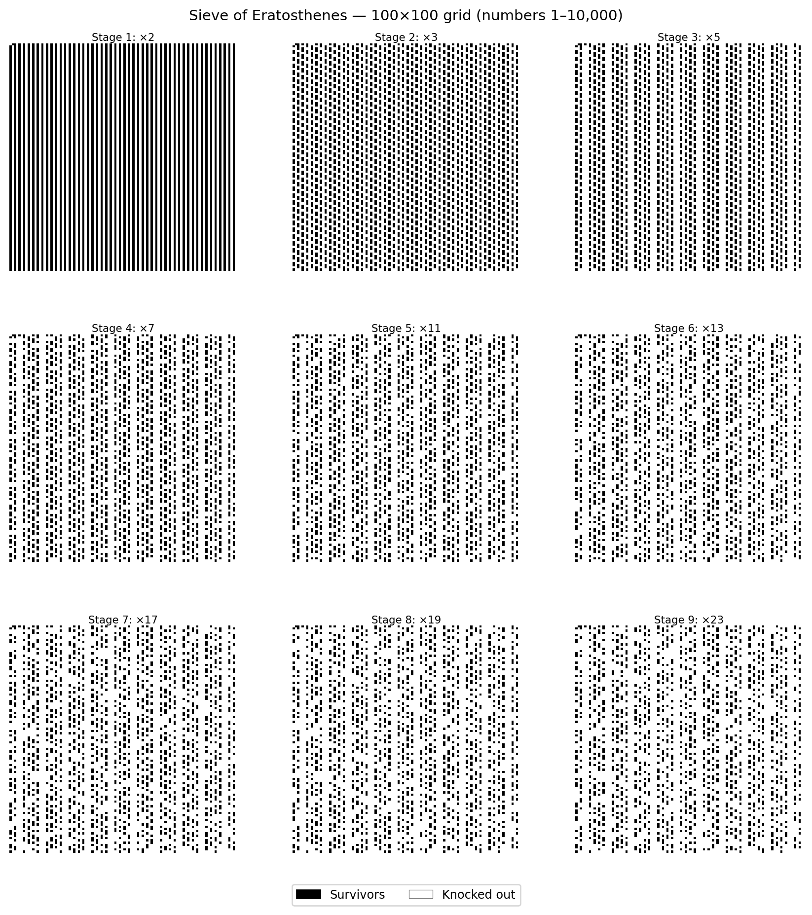
### Research Example: Nine Snapshots of the Sieve {.unnumbered .unlisted}
How does the sieve progressively erase composites, stage by stage? Capture all nine prime-divisor steps in a single grid of panels and watch the board go dark.
```{python}
#| label: fig-sieve-100
#| fig-cap: "Nine cumulative stages of the Sieve of Eratosthenes on all 10,000 integers from 1 to 10,000, arranged in a 100×100 grid. Black cells are Survivors (not yet knocked out); white cells are knocked out. Each stage adds the multiples of the next prime. After Stage 9 (prime 23), the remaining black cells are exactly the primes plus composites whose smallest factor exceeds 23—the first such composite is $29^2 = 841$."
#| fig-align: center
#| out-width: "100%"
import numpy as np
import matplotlib.pyplot as plt
import matplotlib.patches as mpatches

N_GRID = 100
STAGE_PRIMES = [2, 3, 5, 7, 11, 13, 17, 19, 23]

def sieve_stage(primes_used):
    status = np.zeros(N_GRID * N_GRID, dtype=float)
    status[0] = 1.0
    for q in primes_used:
        mul = 2 * q
        while mul <= N_GRID * N_GRID:
            status[mul - 1] = 1.0
            mul += q
    return status.reshape(N_GRID, N_GRID)

fig_snap, axes_snap = plt.subplots(3, 3, figsize=(9, 9.5))
fig_snap.suptitle('Sieve of Eratosthenes — 100×100 grid (numbers 1–10,000)',
                  fontsize=11, y=0.998)

for stage_i, (ax_s, prime_s) in enumerate(zip(axes_snap.flat, STAGE_PRIMES)):
    grid = sieve_stage(STAGE_PRIMES[:stage_i + 1])
    ax_s.imshow(grid, cmap='gray', vmin=0, vmax=1,
                interpolation='nearest', aspect='equal')
    ax_s.set_title(f'Stage {stage_i + 1}: ×{prime_s}', fontsize=8, pad=2)
    ax_s.axis('off')

legend_handles = [
    mpatches.Patch(color='black', label='Survivors'),
    mpatches.Patch(facecolor='white', edgecolor='0.5', linewidth=0.5,
                   label='Knocked out'),
]
fig_snap.legend(handles=legend_handles, loc='lower center', ncol=2,
                fontsize=9, bbox_to_anchor=(0.5, -0.005))
plt.subplots_adjust(left=0.01, right=0.99, top=0.96, bottom=0.06,
                    hspace=0.28, wspace=0.05)
plt.show()
```
Stage 1 already makes the board look half-empty; by Stage 4 the pattern has nearly settled. Watching nine stages side-by-side, you have done in seconds what Eratosthenes did by hand — and spotted something even he may not have quantified.
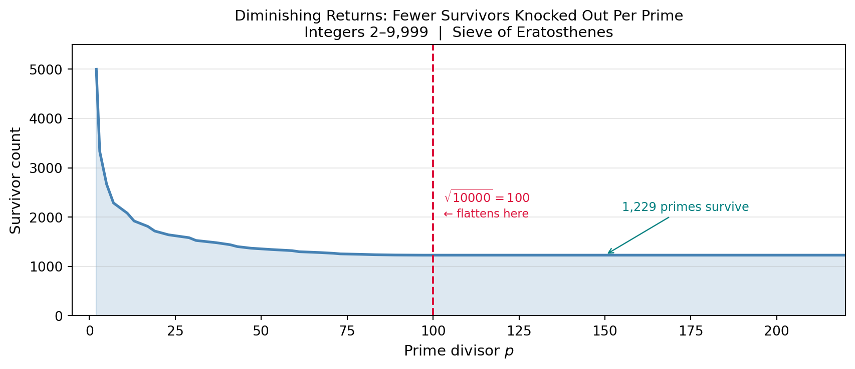
### Research Example: The Sieve's Diminishing Returns {.unnumbered .unlisted}
Does each new prime divisor knock out as many survivors as the one before — or does the sieve's power fade? Plot the survivor count after each prime is applied and measure exactly how fast the payoff shrinks.
```{python}
#| label: fig-sieve-diminishing-returns
#| fig-cap: "Survivor count among integers 2–9,999 as each prime divisor is cumulatively added. Dividing by 2 cuts survivors nearly in half; dividing by 3 removes roughly another third of those; but each successive prime kills a smaller and smaller fraction. After prime 97 — the last prime below $\\sqrt{10{,}000}=100$ — the curve goes completely flat. Every composite below 10,000 has already been eliminated. The survivors at that point are exactly the primes."
#| fig-align: center
#| out-width: "90%"
# uses: sieve()
import numpy as np
import matplotlib.pyplot as plt

N = 10_000
knocked = np.zeros(N + 1, dtype=bool)
knocked[0] = knocked[1] = True

primes_under_N = sieve(N - 1)          # all primes up to 9,999

prime_vals = []
survivor_list = []
for p in primes_under_N:
    knocked[2 * p :: p] = True          # mark new multiples of p
    prime_vals.append(p)
    survivor_list.append(int((~knocked[2:N]).sum()))

n_primes = survivor_list[-1]   # primes below 10,000

fig, ax = plt.subplots(figsize=(9, 4))
ax.fill_between(prime_vals, survivor_list, alpha=0.18, color='steelblue')
ax.plot(prime_vals, survivor_list, color='steelblue', linewidth=2)

ax.axvline(x=100, color='crimson', linestyle='--', linewidth=1.5)
ax.text(103, 2300, r'$\sqrt{10000}=100$', color='crimson', fontsize=9)
ax.text(103, 2000, '← flattens here', color='crimson', fontsize=8.5)

ax.annotate(f'{n_primes:,} primes survive',
            xy=(150, n_primes), xytext=(155, n_primes + 900),
            fontsize=9, color='teal',
            arrowprops=dict(arrowstyle='->', color='teal', lw=0.9))

ax.set_xlim(-5, 220)
ax.set_ylim(0, 5_500)
ax.set_xlabel('Prime divisor $p$', fontsize=11)
ax.set_ylabel('Survivor count', fontsize=11)
ax.set_title(
    'Diminishing Returns: Fewer Survivors Knocked Out Per Prime\n'
    'Integers 2–9,999  |  Sieve of Eratosthenes',
    fontsize=11)
ax.grid(axis='y', alpha=0.3)
fig.tight_layout()
plt.show()
```
The curve flatlines at $p = 97$ — the last prime below $\sqrt{10{,}000} = 100$ — and every composite below 10,000 is already gone. You just proved, in a single graph, why the sieve only needs primes up to the square root. Not bad for a Saturday afternoon with Python.
Notice that the inner loop starts at `i * i`, not at `2 * i`. Every
multiple $m \cdot i$ with $m < i$ has already been crossed off when we
processed the prime $m$ earlier, so starting at $i^2$ saves redundant
work.
```{python}
# uses: sieve()
import time

start = time.perf_counter()
big_primes = sieve(1_000_000)
elapsed = time.perf_counter() - start

print(f"Primes up to 1,000,000: {len(big_primes)}")
print(f"Largest prime found:    {big_primes[-1]}")
print(f"Time elapsed:           {elapsed:.4f} s")
```
The sieve finds all 78,498 primes below one million in a fraction of a
second. That speed will be essential for the experiments later in this
chapter.
## How Fast Is Trial Division? {#sec-primes-trialdiv}
Before we use the sieve, let's build primality testing the hard way — by
hand — just to see how much work it really takes.
The simplest idea: to test whether $n$ is prime, try dividing it by every
integer from 2 up to $n - 1$. If nothing divides evenly, $n$ is prime.
```{python}
def my_isprime(n):
    if n < 2:
        return False
    for i in range(2, n):
        if n % i == 0:
            return False
    return True

for n in [2, 17, 18, 97]:
    print(f"my_isprime({n}) = {my_isprime(n)}")
```
It works. But it is painfully slow for large $n$. How slow? Let's race four
hand-built variants — plus Python's own built-in `isprime` — against the
same large prime, the largest below $100{,}000{,}000$, and find out.
```{python}
#| cache: true
import time
import math
from sympy import primerange, isprime

def my_isprime1(n):
    """Try every integer from 2 to n-1."""
    if n < 2:
        return False
    for i in range(2, n):
        if n % i == 0:
            return False
    return True

def my_isprime2(n):
    """Try every integer from 2 to sqrt(n)."""
    if n < 2:
        return False
    for i in range(2, math.isqrt(n) + 1):
        if n % i == 0:
            return False
    return True

def my_isprime3(n, primes):
    """Try every prime p with p < n."""
    if n < 2:
        return False
    for p in primes:
        if p >= n:
            break
        if n % p == 0:
            return False
    return True

def my_isprime4(n, primes):
    """Try every prime p with p <= sqrt(n)."""
    if n < 2:
        return False
    limit = math.isqrt(n)
    for p in primes:
        if p > limit:
            break
        if n % p == 0:
            return False
    return True

TARGET = 99_999_989        # largest prime below 10^8
prime_list = list(primerange(2, TARGET + 1))

methods = [
    ("all i < n",   my_isprime1, (TARGET,)),
    ("i ≤ √n",      my_isprime2, (TARGET,)),
    ("primes < n",  my_isprime3, (TARGET, prime_list)),
    ("primes ≤ √n", my_isprime4, (TARGET, prime_list)),
    ("isprime",     isprime,     (TARGET,)),
]

timing = []
for label, fn, args in methods:
    t0 = time.perf_counter()
    ok = fn(*args)
    t1 = time.perf_counter()
    timing.append(t1 - t0)
    print(f"{label:13s}: {t1-t0:.4f} s  → {ok}")
```
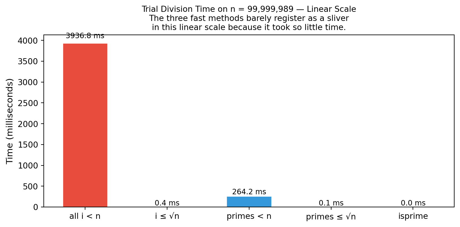
### Research Example: How Much Does Cleverness Matter? {.unnumbered .unlisted}
Five ways to test whether a number is prime — from the obvious brute-force to SymPy's optimized built-in. Race them all on the same large prime and measure exactly how much each optimization saves.
```{python}
#| label: fig-isprime-timing-linear
#| fig-cap: "Trial division timing on a linear scale. The three fast methods are practically invisible next to the first. In order to differentiate them, we will need to switch to a log scale in the next figure."
import matplotlib.pyplot as plt

bar_labels = [
    "all i < n", "i ≤ √n",
    "primes < n", "primes ≤ √n", "isprime",
]
colors = ["#e74c3c", "#e67e22", "#3498db", "#2ecc71", "#9b59b6"]

timing_ms = [t * 1000 for t in timing]

def add_labels(ax, bars, vals_ms):
    for bar, t_ms in zip(bars, vals_ms):
        ax.text(
            bar.get_x() + bar.get_width() / 2,
            bar.get_height() * 1.02,
            f"{t_ms:.1f} ms", ha="center", va="bottom", fontsize=9,
        )

fig, ax = plt.subplots(figsize=(8, 4))
bars = ax.bar(
    bar_labels, timing_ms, color=colors,
    width=0.55, edgecolor="white"
)
ax.set_ylabel("Time (milliseconds)", fontsize=11)
ax.set_title(
    f"Trial Division Time on n = {TARGET:,} — Linear Scale\n"
    "The three fast methods barely register as a sliver\n"
    "in this linear scale because it took so little time.",
    fontsize=10,
)
add_labels(ax, bars, timing_ms)
fig.tight_layout()
plt.show()
```
Notice anything? The three faster bars are essentially invisible — crushed
flat against the bottom by the towering first bar. That is not a plotting
artifact. It is the reality of the numbers. The "smart" methods finish
thousands of times faster, but on a linear scale you simply cannot see them.
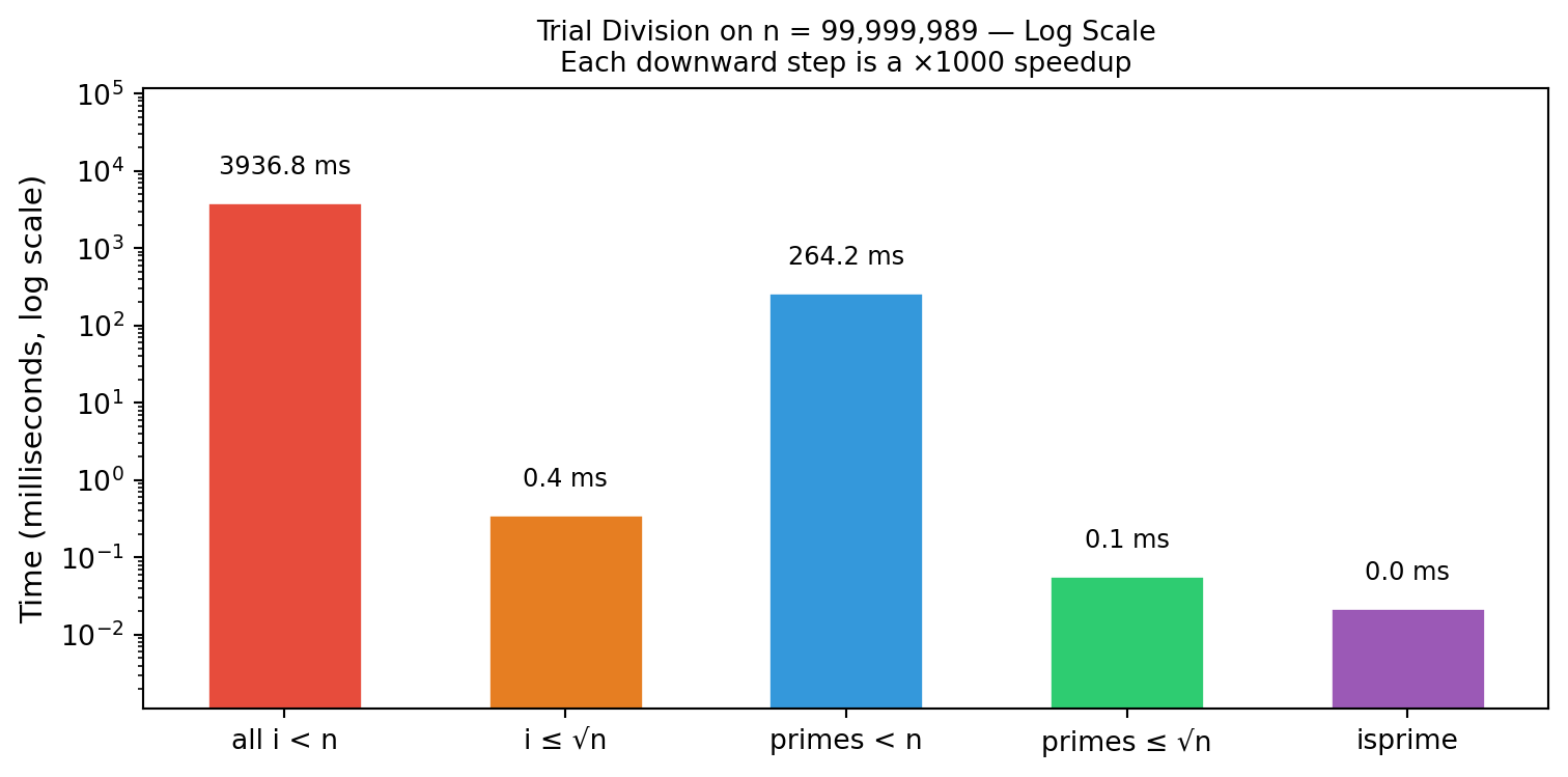
This is exactly the moment to switch to a **log scale**, where each tick
mark represents a ×10 jump instead of a fixed step. Now every bar gets
room to breathe:
```{python}
#| label: fig-isprime-timing-log
#| fig-cap: "Same data on a log scale. Now the improvement at each step is clearly visible."
timing_ms = [t * 1000 for t in timing]
fig, ax = plt.subplots(figsize=(8, 4))
bars = ax.bar(
    bar_labels, timing_ms, color=colors,
    width=0.55, edgecolor="white"
)
ax.set_yscale("log")
ax.set_ylabel("Time (milliseconds, log scale)", fontsize=11)
ax.set_title(
    f"Trial Division on n = {TARGET:,} — Log Scale\n"
    "Each downward step is a ×1000 speedup",
    fontsize=10,
)
for bar, t_ms in zip(bars, timing_ms):
    ax.text(
        bar.get_x() + bar.get_width() / 2,
        bar.get_height() * 2,
        f"{t_ms:.1f} ms", ha="center", va="bottom", fontsize=9,
    )
ax.set_ylim(min(timing_ms) * 0.05, max(timing_ms) * 30)
fig.tight_layout()
plt.show()
```
One geometric insight — *stop at the square root* — transforms a years-long computation into a millisecond one. You built that insight from scratch in twenty lines, and that is exactly the kind of question-then-measurement loop that drives real algorithmic research.
## The Prime-Counting Function {#sec-primes-count}
```{python}
#| echo: false
from pathlib import Path; import urllib.request
_d = Path('images'); _d.mkdir(exist_ok=True)
_p = _d / 'gauss.jpg'
if not _p.exists():
try: urllib.request.urlretrieve('https://upload.wikimedia.org/wikipedia/commons/9/9b/Carl_Friedrich_Gauss.jpg', _p)
except Exception: pass
```
::: {.content-visible when-format="pdf"}
```{=latex}
\begin{center}
\begin{minipage}[c]{0.22\textwidth}
\includegraphics[width=\textwidth]{images/gauss.jpg}
\end{minipage}%
\hspace{0.03\textwidth}%
\begin{minipage}[c]{0.35\textwidth}
\small\textit{Carl Friedrich Gauss (1777--1855)}\\[2pt]
\tiny Public domain
\end{minipage}
\end{center}
```
:::
::: {.content-visible when-format="html"}
<div style="display:flex; align-items:center; margin:1em 0; gap:12px;">
<img src="images/gauss.jpg" style="width:100px; flex-shrink:0;" alt="Carl Friedrich Gauss">
<div style="font-size:0.82em;"><em>Carl Friedrich Gauss (1777–1855)</em><br><span style="font-size:0.85em;">Public domain</span></div>
</div>
:::
Let $\pi(x)$ denote the number of primes less than or equal to $x$ (the
$\pi$ here is a function name, not the constant $3.14159\ldots$). The
first few values are $\pi(2) = 1$, $\pi(10) = 4$, $\pi(100) = 25$.
How does $\pi(x)$ grow? The **Prime Number Theorem** (PNT), proved
independently by Hadamard and de la Vallée Poussin in 1896 [@hardywright1979], states that:
$$\pi(x) \sim \frac{x}{\ln x} \quad \text{as } x \to \infty$$
The symbol $\sim$ means the ratio $\pi(x) / (x / \ln x)$ approaches $1$.
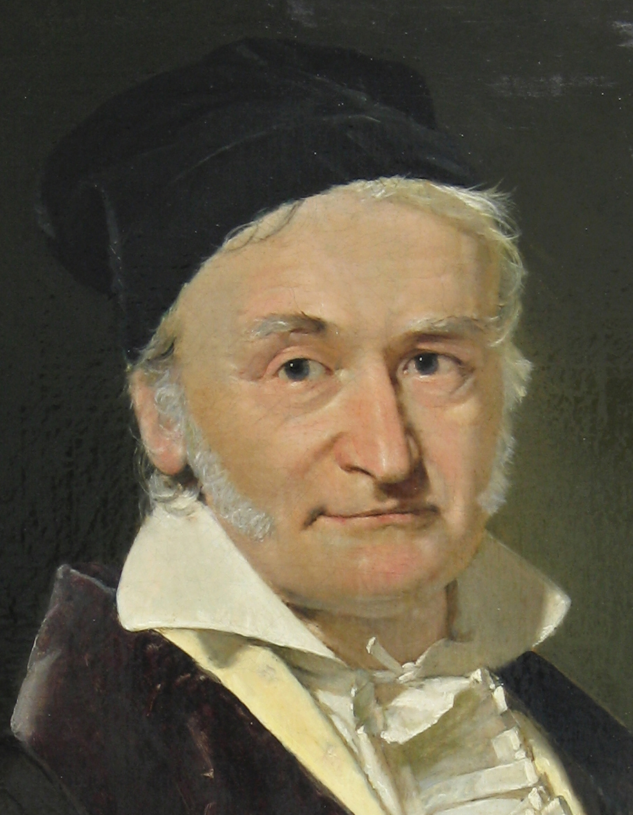
Gauss conjectured this relationship around 1792, when he was a teenager,
by staring at tables of primes.
### Research Example: Did Gauss Get It Right? {.unnumbered .unlisted}
Gauss claimed that $x / \ln x$ tracks the prime count — but how close is it, really? Plot both curves together and see for yourself whether a teenager's conjecture from 1792 holds up.
```{python}
# uses: sieve()
import matplotlib.pyplot as plt
import math

plt.style.use('default')

limit = 2000
all_primes = sieve(limit)
prime_set = set(all_primes)

x_vals = list(range(2, limit + 1))
pi_vals = []
count = 0
for x in x_vals:
    if x in prime_set:
        count += 1
    pi_vals.append(count)

gauss = [x / math.log(x) for x in x_vals]

fig, ax = plt.subplots(figsize=(7, 4))
ax.plot(x_vals, pi_vals, label=r"$\pi(x)$")
ax.plot(
    x_vals, gauss, '--', color='orange',
    label=r"$x / \ln x$"
)
ax.set_xlabel("x")
ax.set_ylabel("count")
ax.set_title(
    "Prime-Counting Function and "
    "the Gauss Approximation"
)
ax.legend()
fig.tight_layout()
plt.show()
```
Gauss was right: $x / \ln x$ shadows the real count closely, though it consistently underestimates near the origin. A teenager staring at prime tables spotted a theorem that took over a century to prove — and you just reproduced his observation in a dozen lines of Python.
## Prime Gaps {#sec-primes-gaps}
```{python}
#| echo: false
from pathlib import Path; import urllib.request
_d = Path('images'); _d.mkdir(exist_ok=True)
_p = _d / 'riemann.jpg'
if not _p.exists():
try: urllib.request.urlretrieve('https://upload.wikimedia.org/wikipedia/commons/8/82/Georg_Friedrich_Bernhard_Riemann.jpeg', _p)
except Exception: pass
```
::: {.content-visible when-format="pdf"}
```{=latex}
\begin{center}
\begin{minipage}[c]{0.22\textwidth}
\includegraphics[width=\textwidth]{images/riemann.jpg}
\end{minipage}%
\hspace{0.03\textwidth}%
\begin{minipage}[c]{0.35\textwidth}
\small\textit{Bernhard Riemann (1826--1866)}\\[2pt]
\tiny Public domain
\end{minipage}
\end{center}
```
:::
::: {.content-visible when-format="html"}
<div style="display:flex; align-items:center; margin:1em 0; gap:12px;">
<img src="images/riemann.jpg" style="width:100px; flex-shrink:0;" alt="Bernhard Riemann">
<div style="font-size:0.82em;"><em>Bernhard Riemann (1826–1866)</em><br><span style="font-size:0.85em;">Public domain</span></div>
</div>
:::
The **gap** between consecutive primes $p$ and $q$ (the next prime after
$p$) is simply $q - p$. Small gaps like $2$ (twin primes: $3, 5$ or
$11, 13$) appear endlessly as far as we can compute, though no one has
proved there are infinitely many.
Large gaps also appear. By a simple argument: for any $k \geq 2$, the $k$
consecutive integers $k!+2,\ k!+3,\ \ldots,\ k!+k$ are all composite
(the $j$-th one is divisible by $j$). So prime gaps can be arbitrarily
large. But where do they actually occur?
```{python}
# uses: sieve()
primes_10k = sieve(10_000)
gaps = [
    primes_10k[i + 1] - primes_10k[i]
    for i in range(len(primes_10k) - 1)
]

n = len(primes_10k)
total = sum(gaps)
print(f"Primes up to 10,000:  {n}")
print(f"Largest gap:          {max(gaps)}")
print(f"Average gap:          {total / len(gaps):.2f}")
```
```{python}
top5 = sorted(
    enumerate(gaps), key=lambda t: t[1],
    reverse=True
)[:5]
print("Five largest prime gaps below 10,000:")
for idx, g in top5:
    p = primes_10k[idx]
    q = primes_10k[idx + 1]
    print(f"  {p} to {q}: gap = {g}")
```
The average gap near $x$ is approximately $\ln x$ by the PNT (since
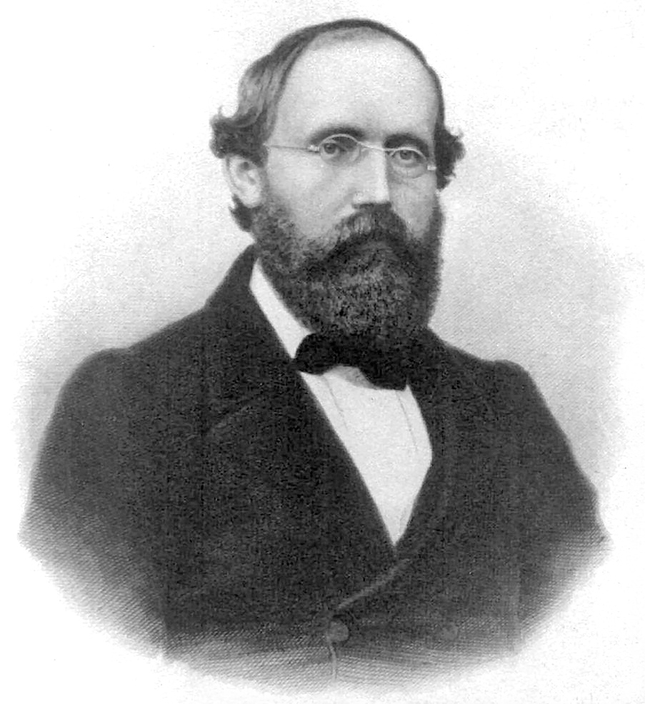
primes thin out at that rate). Bernhard Riemann's landmark 1859 paper [@riemann1859]
showed that the precise statistics of prime gaps are encoded in the zeros
of a complex function; exactly where those zeros lie is the Riemann
Hypothesis, the most famous unsolved problem in mathematics.
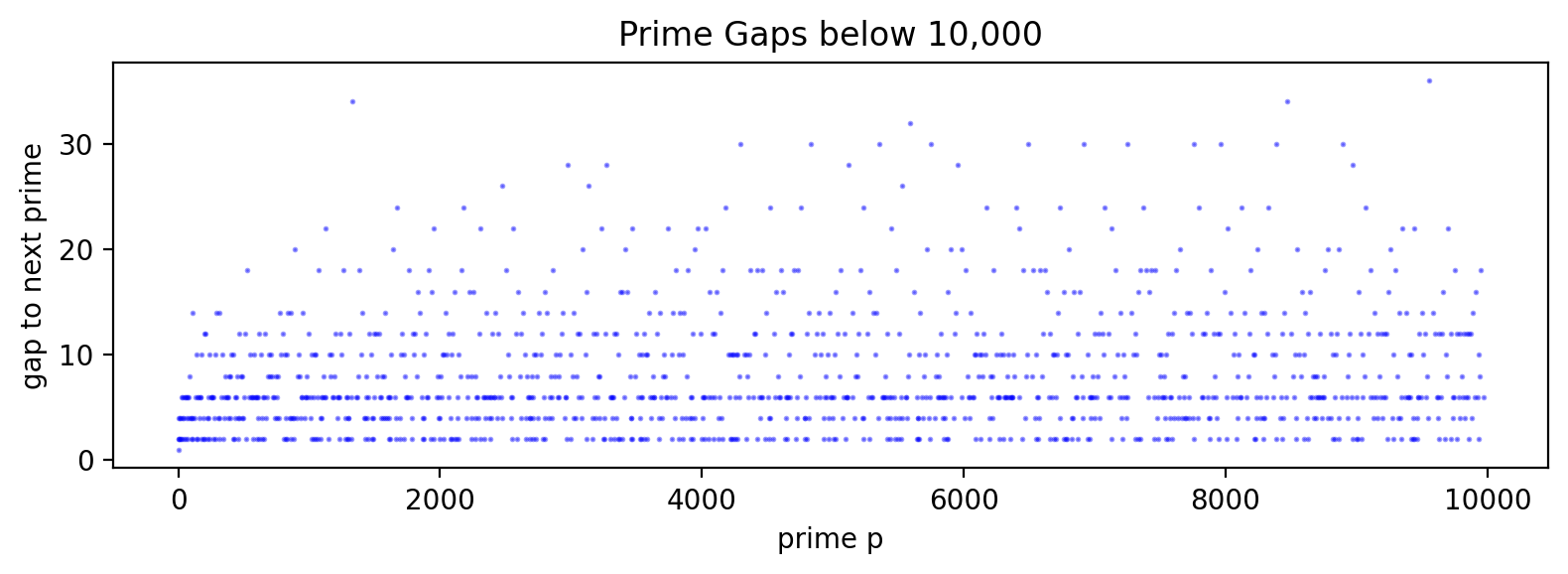
### Research Example: Do Prime Gaps Grow Forever? {.unnumbered .unlisted}
We know primes thin out, so gaps should grow — but does the scatter plot actually show that trend, or is it hidden in noise? Plot every gap below 10,000 against its starting prime and find out.
```{python}
# uses: primes_10k, gaps
import matplotlib.pyplot as plt

fig, ax = plt.subplots(figsize=(8, 3))
ax.scatter(
    primes_10k[:-1], gaps,
    s=1, alpha=0.4, color='blue'
)
ax.set_xlabel("prime p")
ax.set_ylabel("gap to next prime")
ax.set_title("Prime Gaps below 10,000")
fig.tight_layout()
plt.show()
```
The upward drift is unmistakable — gaps really do grow as primes get larger, just as the Prime Number Theorem predicts. You have turned an abstract theorem about logarithms into a pattern you can see with your own eyes.
```{python}
#| echo: false
from pathlib import Path
import urllib.request
_d = Path('images'); _d.mkdir(exist_ok=True)
_p = _d / 'thumb_D4_sNKoO-RA.jpg'
try:
if not _p.exists():
urllib.request.urlretrieve('https://img.youtube.com/vi/D4_sNKoO-RA/0.jpg', _p)
except Exception:
pass
```
::: {.content-visible when-format="pdf"}
```{=latex}
\begin{center}
\begin{minipage}[c]{0.28\textwidth}
\centering
\href{https://youtu.be/D4_sNKoO-RA}{\includegraphics[width=\textwidth]{images/thumb_D4_sNKoO-RA.jpg}}
\end{minipage}%
\hspace{0.02\textwidth}%
\begin{minipage}[c]{0.28\textwidth}
\small\textbf{Numberphile}\\[3pt]
\small Gaps between Primes (extra footage)\\[3pt]
\small\href{https://youtu.be/D4_sNKoO-RA}{\texttt{youtu.be/D4\_sNKoO-RA}}
\end{minipage}%
\hspace{0.02\textwidth}%
\begin{minipage}[c]{0.36\textwidth}
\small Extra footage exploring why prime gaps grow without bound and what statistical patterns emerge in their distribution.
\end{minipage}
\end{center}
```
:::
::: {.content-visible when-format="html"}
<div style="display:flex; align-items:flex-start; margin:1em 0; gap:12px; width:100%;">
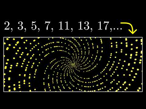
<div style="flex:0 0 200px;"><a href="https://youtu.be/D4_sNKoO-RA" target="_blank"><img src="https://img.youtube.com/vi/D4_sNKoO-RA/0.jpg" style="width:100%;display:block;" alt="Gaps between Primes (extra footage)"></a></div>
<div style="flex:1; font-size:0.85em;"><strong>Numberphile</strong><br>Gaps between Primes (extra footage)<br><a href="https://youtu.be/D4_sNKoO-RA" target="_blank" style="font-family:Consolas,monospace;">youtu.be/D4_sNKoO-RA</a></div>
<div style="flex:1; font-size:0.85em;">Extra footage exploring why prime gaps grow without bound and what statistical patterns emerge in their distribution.</div>
</div>
:::
The scatter plot reveals a fan-shaped pattern: as primes grow larger,
the maximum gap grows, but small gaps like $2$ persist throughout. Notice
also that almost all gaps are even (since both endpoints are odd primes),
so the data collapses onto horizontal lines at $2, 4, 6, 8, \ldots$
## Goldbach's Conjecture {#sec-primes-goldbach}
```{python}
#| echo: false
from pathlib import Path; import urllib.request
_d = Path('images'); _d.mkdir(exist_ok=True)
for _url, _fn in [
('https://upload.wikimedia.org/wikipedia/commons/d/d7/Leonhard_Euler.jpg', 'euler.jpg'),
('https://explainingscience.org/wp-content/uploads/2019/08/goldbachgoldbach-1.png', 'goldbach.png'),
]:
_p = _d / _fn
if not _p.exists():
try:
_req = urllib.request.Request(_url, headers={'User-Agent': 'Mozilla/5.0'})
with urllib.request.urlopen(_req) as _r:
_p.write_bytes(_r.read())
except Exception: pass
```
::: {.content-visible when-format="pdf"}
```{=latex}
\begin{center}
\begin{minipage}[c]{0.20\textwidth}
\includegraphics[width=\textwidth]{images/goldbach.png}
\end{minipage}%
\hspace{0.02\textwidth}%
\begin{minipage}[c]{0.23\textwidth}
\small\textit{Christian Goldbach (1690--1764)}\\[2pt]
\tiny Public domain
\end{minipage}%
\hspace{0.04\textwidth}%
\begin{minipage}[c]{0.20\textwidth}
\includegraphics[width=\textwidth]{images/euler.jpg}
\end{minipage}%
\hspace{0.02\textwidth}%
\begin{minipage}[c]{0.23\textwidth}
\small\textit{Leonhard Euler (1707--1783)}\\[2pt]
\tiny Public domain
\end{minipage}
\end{center}
```
:::
::: {.content-visible when-format="html"}
<div style="display:flex; align-items:center; margin:1em 0; gap:16px;">
<img src="images/goldbach.png" style="width:90px; flex-shrink:0;" alt="Christian Goldbach">
<div style="font-size:0.82em;"><em>Christian Goldbach (1690–1764)</em><br><span style="font-size:0.85em;">Public domain</span></div>
<img src="images/euler.jpg" style="width:90px; flex-shrink:0; margin-left:16px;" alt="Leonhard Euler">
<div style="font-size:0.82em;"><em>Leonhard Euler (1707–1783)</em><br><span style="font-size:0.85em;">Public domain</span></div>
</div>
:::
In a 1742 letter to Euler, Christian Goldbach observed that every even
integer he tested could be written as a sum of two primes:
$$4 = 2+2, \quad 6 = 3+3, \quad 8 = 3+5, \quad 10 = 3+7 = 5+5,
\quad \ldots$$
**Goldbach's Conjecture**: Every even integer $n \geq 4$ is the sum of two
primes [@goldbach1742].
This conjecture is 280 years old and still unproven. It has been verified
by computer for all even numbers up to $4 \times 10^{18}$ [@oliveira2014], but no proof
exists. It is one of the most famous open problems in mathematics.
Let us verify it for small values and count how many ways each even number
can be decomposed.
```{python}
from sympy import isprime

def goldbach_pairs(n):
    """
    Return all pairs (p, q) with p <= q,
    p + q = n, both prime.
    n must be an even integer >= 4.
    """
    pairs = []
    for p in range(2, n // 2 + 1):
        if isprime(p) and isprime(n - p):
            pairs.append((p, n - p))
    return pairs

for n in range(4, 24, 2):
    pairs = goldbach_pairs(n)
    print(f"{n:3d}: {pairs}")
```
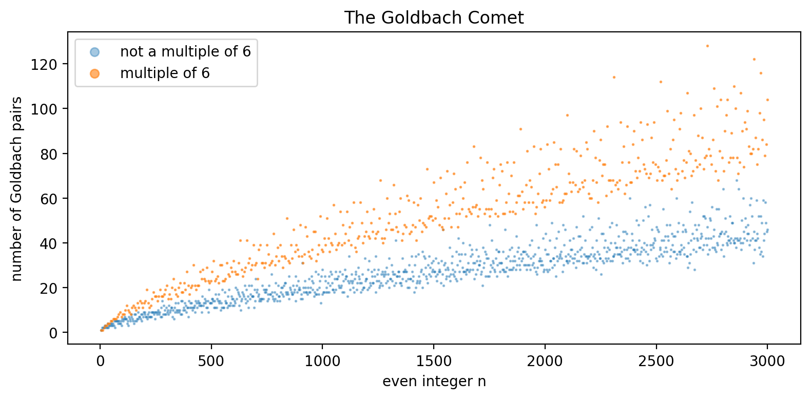
### Research Example: The Goldbach Comet {.unnumbered .unlisted}
Every even number seems expressible as a sum of two primes — but does the *number* of such representations grow, shrink, or scatter randomly as $n$ increases? Plot the representation count for every even number up to 3,000 and discover one of mathematics' most striking shapes.
```{python}
# uses: sieve()
import matplotlib.pyplot as plt

limit = 3000
all_primes = sieve(limit)
prime_set = set(all_primes)

even_ns = list(range(4, limit + 1, 2))
counts = []
for n in even_ns:
    c = 0
    for p in all_primes:
        if p > n // 2:
            break
        if (n - p) in prime_set:
            c += 1
    counts.append(c)

ORANGE = '#ff7f0e'
BLUE   = '#1f77b4'

mult6_x = [n for n in even_ns if n % 6 == 0]
mult6_y = [c for n, c in zip(even_ns, counts) if n % 6 == 0]
rest_x  = [n for n in even_ns if n % 6 != 0]
rest_y  = [c for n, c in zip(even_ns, counts) if n % 6 != 0]

fig, ax = plt.subplots(figsize=(8, 4))
ax.scatter(rest_x,  rest_y,  s=1, alpha=0.4, color=BLUE,   label='not a multiple of 6')
ax.scatter(mult6_x, mult6_y, s=1, alpha=0.6, color=ORANGE, label='multiple of 6')
ax.set_xlabel("even integer n")
ax.set_ylabel("number of Goldbach pairs")
ax.set_title("The Goldbach Comet")
ax.legend(markerscale=6, loc='upper left')
fig.tight_layout()
plt.show()
```
Two branches, one for multiples of 6 and one for the rest, streak upward together like a comet's tail. You just visualized an unsolved problem — and produced research-quality data with thirty lines of Python.
## The Ulam Spiral {#sec-primes-ulam}
```{python}
#| echo: false
from pathlib import Path; import urllib.request
_d = Path('images'); _d.mkdir(exist_ok=True)
_p = _d / 'ulam.png'
if not _p.exists():
try: urllib.request.urlretrieve('https://upload.wikimedia.org/wikipedia/commons/b/be/Stanislaw_Ulam_ID_badge.png', _p)
except Exception: pass
```
::: {.content-visible when-format="pdf"}
```{=latex}
\begin{center}
\begin{minipage}[c]{0.22\textwidth}
\includegraphics[width=\textwidth]{images/ulam.png}
\end{minipage}%
\hspace{0.03\textwidth}%
\begin{minipage}[c]{0.35\textwidth}
\small\textit{Stanislaw Ulam (1909--1984)}\\[2pt]
\tiny Los Alamos Natl. Lab.; public domain
\end{minipage}
\end{center}
```
:::
::: {.content-visible when-format="html"}
<div style="display:flex; align-items:center; margin:1em 0; gap:12px;">
<img src="images/ulam.png" style="width:100px; flex-shrink:0;" alt="Stanislaw Ulam">
<div style="font-size:0.82em;"><em>Stanislaw Ulam (1909–1984)</em><br><span style="font-size:0.85em;">Los Alamos Natl. Lab.; public domain</span></div>
</div>
:::
In 1963, the mathematician Stanislaw Ulam was sitting through a boring
meeting and began doodling: he wrote the integers in a spiral on grid
paper and circled all the primes. To his surprise, the circled numbers
lined up along diagonal stripes. The pattern was too pronounced to be
coincidence. Ulam (1909–1984) was a Polish-American mathematician
whose other major contributions include the Monte Carlo method and
nuclear weapon design --- a reminder that mathematical discovery can
emerge from the most unexpected moments.
The **Ulam spiral** arranges integers $1, 2, 3, \ldots$ in a square spiral
centered at $1$, then marks which positions are prime. We will build it
with NumPy and display it with `imshow`.
```{python}
import numpy as np

def ulam_spiral(size):
    """
    Return a (2*size+1) x (2*size+1) NumPy
    array with integers arranged in Ulam
    spiral order. 1 is at the center.
    """
    n = 2 * size + 1
    grid = np.zeros((n, n), dtype=int)
    r, c = size, size
    grid[r, c] = 1
    num = 2
    step = 1
    dr = [0, -1, 0,  1]   # right, up, left, down
    dc = [1,  0, -1, 0]
    d = 0
    while num <= n * n:
        for _ in range(2):
            for _ in range(step):
                if num > n * n:
                    break
                r += dr[d]
                c += dc[d]
                grid[r, c] = num
                num += 1
            d = (d + 1) % 4
        step += 1
    return grid

spiral = ulam_spiral(100)   # 201 x 201 grid
print(f"Grid size:    {spiral.shape}")
print(f"Center value: {spiral[100, 100]}")
print(f"Max value:    {spiral.max()}")
```
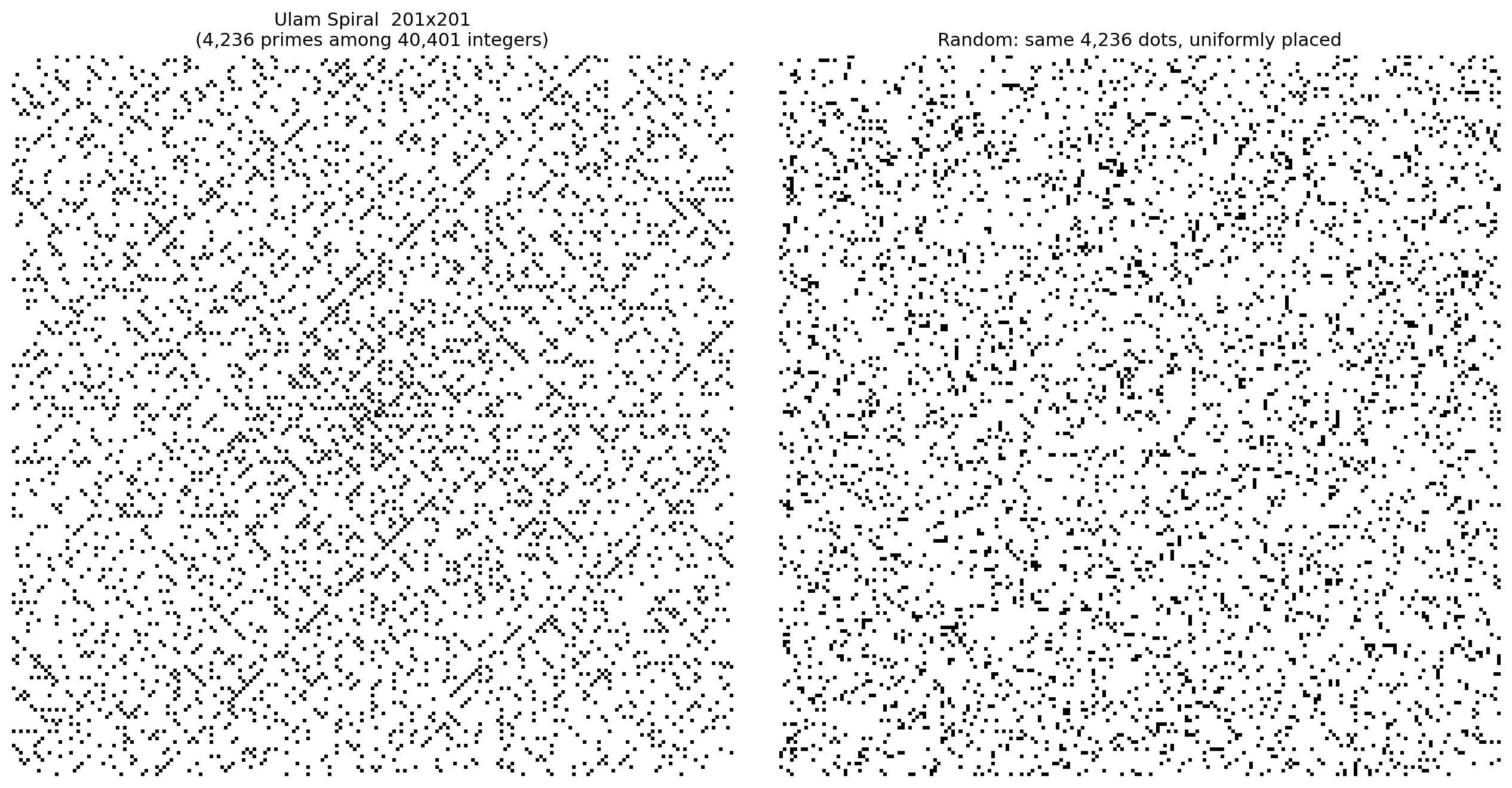
### Research Example: Do Primes Line Up? {.unnumbered .unlisted}
If primes were truly "random," they should scatter uniformly in any arrangement — but the Ulam spiral suggests otherwise. Build the spiral, mark every prime, and place the same number of random dots beside it; let the contrast speak for itself.
```{python}
#| label: fig-ulam-200
#| fig-cap: "Left: Ulam spiral, 201×201 grid (numbers 1 to 40,401). Black dots mark prime positions. Diagonal streaks arise because certain quadratic polynomials produce prime values unusually often. Right: the same number of dots placed at uniformly random positions — no structure appears."
#| fig-align: center
#| out-width: "100%"
# uses: spiral
import numpy as np
import matplotlib.pyplot as plt
from sympy import isprime

prime_mask = np.vectorize(isprime)(spiral)
n_primes = int(prime_mask.sum())
n = spiral.shape[0]

rng = np.random.default_rng(42)
flat = np.zeros(n * n, dtype=bool)
flat[rng.choice(n * n, size=n_primes, replace=False)] = True
random_mask = flat.reshape(n, n)

fig, (ax1, ax2) = plt.subplots(1, 2, figsize=(13, 6.5))
ax1.imshow(~prime_mask, cmap='gray', interpolation='nearest')
ax1.set_title(
    f'Ulam Spiral  {n}x{n}\n({n_primes:,} primes among {n*n:,} integers)',
    fontsize=11)
ax1.axis('off')
ax2.imshow(~random_mask, cmap='gray', interpolation='nearest')
ax2.set_title(
    f'Random: same {n_primes:,} dots, uniformly placed',
    fontsize=11)
ax2.axis('off')
fig.tight_layout()
plt.show()
```
Left panel: diagonal stripes that nobody planted. Right panel: pure noise. Primes are not random — they are governed by hidden structure that even a bored doodler can discover. You now hold the same image that launched a research program in the 1960s.
```{python}
#| echo: false
from pathlib import Path
import urllib.request
_d = Path('images'); _d.mkdir(exist_ok=True)
for _vid in ['EK32jo7i5LQ', 'iFuR97YcSLM']:
_p = _d / f'thumb_{_vid}.jpg'
try:
if not _p.exists():
urllib.request.urlretrieve(f'https://img.youtube.com/vi/{_vid}/0.jpg', _p)
except Exception:
pass
```
::: {.content-visible when-format="pdf"}
```{=latex}
\begin{center}
\begin{minipage}[c]{0.28\textwidth}
\centering
\href{https://youtu.be/EK32jo7i5LQ}{\includegraphics[width=\textwidth]{images/thumb_EK32jo7i5LQ.jpg}}
\end{minipage}%
\hspace{0.02\textwidth}%
\begin{minipage}[c]{0.28\textwidth}
\small\textbf{3Blue1Brown}\\[3pt]
\small Why do prime numbers make these spirals?\\[3pt]
\small\href{https://youtu.be/EK32jo7i5LQ}{\texttt{youtu.be/EK32jo7i5LQ}}
\end{minipage}%
\hspace{0.02\textwidth}%
\begin{minipage}[c]{0.36\textwidth}
\small Reveals the spoke pattern that appears when primes are plotted in polar coordinates and connects it to Dirichlet's theorem on primes in arithmetic progressions.
\end{minipage}
\end{center}
```
:::
::: {.content-visible when-format="html"}
<div style="display:flex; align-items:flex-start; margin:1em 0; gap:12px; width:100%;">
<div style="flex:0 0 200px;"><a href="https://youtu.be/EK32jo7i5LQ" target="_blank"><img src="https://img.youtube.com/vi/EK32jo7i5LQ/0.jpg" style="width:100%;display:block;" alt="Why do prime numbers make these spirals?"></a></div>
<div style="flex:1; font-size:0.85em;"><strong>3Blue1Brown</strong><br>Why do prime numbers make these spirals?<br><a href="https://youtu.be/EK32jo7i5LQ" target="_blank" style="font-family:Consolas,monospace;">youtu.be/EK32jo7i5LQ</a></div>
<div style="flex:1; font-size:0.85em;">Reveals the spoke pattern that appears when primes are plotted in polar coordinates and connects it to Dirichlet's theorem on primes in arithmetic progressions.</div>
</div>
:::
::: {.content-visible when-format="pdf"}
```{=latex}
\begin{center}
\begin{minipage}[c]{0.28\textwidth}
\centering
\href{https://youtu.be/iFuR97YcSLM}{\includegraphics[width=\textwidth]{images/thumb_iFuR97YcSLM.jpg}}
\end{minipage}%
\hspace{0.02\textwidth}%
\begin{minipage}[c]{0.28\textwidth}
\small\textbf{Numberphile}\\[3pt]
\small Prime Spirals\\[3pt]
\small\href{https://youtu.be/iFuR97YcSLM}{\texttt{youtu.be/iFuR97YcSLM}}
\end{minipage}%
\hspace{0.02\textwidth}%
\begin{minipage}[c]{0.36\textwidth}
\small Shows the Ulam spiral — primes arranged in a square grid — and explains why they cluster along diagonal lines rather than scattering randomly.
\end{minipage}
\end{center}
```
:::
::: {.content-visible when-format="html"}
<div style="display:flex; align-items:flex-start; margin:1em 0; gap:12px; width:100%;">
<div style="flex:0 0 200px;"><a href="https://youtu.be/iFuR97YcSLM" target="_blank"><img src="https://img.youtube.com/vi/iFuR97YcSLM/0.jpg" style="width:100%;display:block;" alt="Prime Spirals"></a></div>
<div style="flex:1; font-size:0.85em;"><strong>Numberphile</strong><br>Prime Spirals<br><a href="https://youtu.be/iFuR97YcSLM" target="_blank" style="font-family:Consolas,monospace;">youtu.be/iFuR97YcSLM</a></div>
<div style="flex:1; font-size:0.85em;">Shows the Ulam spiral — primes arranged in a square grid — and explains why they cluster along diagonal lines rather than scattering randomly.</div>
</div>
:::
The diagonal streaks are unmistakable. They arise because certain
quadratic polynomials like $4n^2 - 2n + 41$ produce prime values
unusually often, and those polynomials correspond to diagonals in the
spiral. Euler famously noticed that $n^2 + n + 41$ is prime for every
$n = 0, 1, \ldots, 39$ --- an extraordinary run, though it eventually
fails at $n = 40$.
What looked like random scatter in a boring meeting turned out to have
deep structure. That is experimental mathematics at its best.
## Further Research Topics {#sec-primes-research}
The following topics are listed roughly in order of increasing difficulty.
Each one is a genuine open-ended investigation: start by experimenting with
small cases, look for patterns, state a conjecture, then try to explain
what you see.
**1. Twin primes and their density.**
A *twin prime pair* is a pair $(p, p+2)$ where both are prime, such as
$(11, 13)$ or $(41, 43)$. Write code to collect all twin prime pairs up to
$10^6$. Plot the cumulative count of twin primes up to $x$ alongside
$\pi(x)$ on the same axes. Does the twin prime count seem to grow at a
similar rate, a slower rate, or much slower? The **Twin Prime Conjecture**
--- that there are infinitely many --- is unproven.
*(Problem proposed by Claude Code.)*
**2. Mersenne primes.**
A *Mersenne prime* is a prime of the form $2^p - 1$. Show algebraically
that if $2^p - 1$ is prime then $p$ itself must be prime (hint: factor
$2^{ab} - 1$). Use the sieve to check which $p \leq 61$ yield a Mersenne
prime. The largest known primes are almost always Mersenne primes --- why
do you think that is?
*(Problem proposed by Claude Code.)*
**3. The Prime Number Theorem ratio.**
The PNT says $\pi(x) \cdot \ln(x) / x \to 1$. Plot this ratio for
$x = 100, 200, \ldots, 10^6$ (use the sieve for speed). How quickly does
it approach $1$? A better approximation is the logarithmic integral
$\text{Li}(x)$; SymPy provides it as `sympy.li`. Add $\text{Li}(x)$ to
your plot and compare the two approximations.
*(Problem proposed by Claude Code.)*
**4. Goldbach comet to 100,000.**
Extend the Goldbach comet from this chapter to even numbers up to
$100{,}000$ (use the sieve, not `isprime` in a loop). The two main branches
become clearer at this scale. Investigate: do even numbers divisible by
$6$ consistently have more representations? Explain why by thinking about
remainders modulo $6$.
*(Problem proposed by Claude Code.)*
**5. Legendre's conjecture.**
Adrien-Marie Legendre conjectured that there is always at least one prime
between $n^2$ and $(n+1)^2$ for every positive integer $n$. This is still
unproven [@hardywright1979]. Verify it computationally for $n = 1, 2, \ldots, 500$. For each
$n$, record *how many* primes fall in the interval. Does the count grow?
At roughly what rate?
*(Problem proposed by Claude Code.)*
**6. Bertrand's postulate.**
Bertrand's postulate [@hardywright1979] (proved by Chebyshev in 1852) states that for every
integer $n \geq 1$ there is always a prime $p$ with $n < p \leq 2n$.
Verify this for $n = 1$ through $10{,}000$. For each $n$, find the
*smallest* prime in the interval $(n, 2n]$. How close to $n$ does it tend
to fall? Plot the ratio (smallest such prime)$/n$ as a function of $n$.
*(Problem proposed by Claude Code.)*
**7. Cousin and sexy primes.**
Primes that differ by $4$ are called *cousin primes* (e.g., $3$ and $7$);
primes that differ by $6$ are called *sexy primes* (e.g., $5$ and $11$).
Count cousin prime pairs and sexy prime pairs up to $10^6$ and compare
their counts with twin prime pairs. Which gap size ($2$, $4$, or $6$)
produces the most pairs? Can you explain the pattern using modular
arithmetic modulo $6$? (Hint: every prime $> 3$ is either $\equiv 1$ or
$\equiv 5 \pmod 6$.)
*(Problem proposed by Claude Code.)*
**8. Euler's prime-generating polynomial and the Ulam spiral.**
Euler observed that $f(n) = n^2 + n + 41$ is prime for $n = 0, 1, \ldots,
39$. Verify this. Find the diagonal in the Ulam spiral that corresponds to
this polynomial. Now search for other quadratic polynomials
$f(n) = an^2 + bn + c$ (with small positive integer coefficients) that
produce an unusually long run of prime values. Which polynomial gives the
longest run for $n = 0, 1, \ldots, 99$? There is a deep connection between
long prime-producing runs and the diagonals visible in the Ulam spiral.
*(Problem proposed by Claude Code.)*
**9. Primorial primes and Euclid's construction.**
The product of the first $k$ primes is the $k$-th *primorial*, written
$p_k\#$. For example $5\# = 2 \cdot 3 \cdot 5 = 30$. Euclid's
infinitely-many-primes proof produces the numbers $p_k\# + 1$. Check
whether $p_k\# + 1$ is prime for the first ten primorials; when it is
composite, find its smallest prime factor. Repeat for $p_k\# - 1$. Primes
of either form are called *primorial primes*. Does $p_k\# + 1$ being prime
seem to be the common case or the rare exception?
*(Problem proposed by Claude Code.)*
**10. Wilson's theorem as a primality test.**
Wilson's theorem [@hardywright1979] states: $n > 1$ is prime *if and only if*
$(n-1)! \equiv -1 \pmod{n}$. Verify this for all $n \leq 30$ using
Python's `pow(factorial(n-1), 1, n)` (SymPy's `factorial` is exact).
This gives a mathematically perfect criterion for primality --- yet
it is completely useless in practice. Estimate how many multiplications
are needed to test a 20-digit number by Wilson's theorem versus trial
division versus `sympy.isprime`. By how many orders of magnitude does
Wilson's method lose?
*(Problem proposed by Claude Code.)*
**11. Sophie Germain primes and safe primes.**
A prime $p$ is a *Sophie Germain prime* if $2p + 1$ is also prime; the
companion $2p + 1$ is then called a *safe prime*. For example $p = 11$:
$2(11) + 1 = 23$, both prime. Find all Sophie Germain primes up to
$10^6$. Plot their cumulative count alongside twin primes on the same
axes. Which grows faster? Sophie Germain primes were used historically in
attempts to prove Fermat's Last Theorem, and safe primes appear in
modern cryptographic key generation --- briefly research why.
*(Problem proposed by Claude Code.)*
**12. Emirps and palindromic primes.**
An *emirp* is a prime $p$ whose digit-reversal is a *different* prime,
such as $13 \to 31$. A *palindromic prime* reads the same forward and
backward, like $11$, $101$, $10301$. Find all emirps and palindromic
primes below $10^6$. Which is more common? Now prove (or disprove by
counterexample): a palindromic prime with an *even* number of digits must
be divisible by $11$. (Hint: recall the divisibility rule for $11$.) What
does this say about even-digit palindromic primes $> 11$?
*(Problem proposed by Claude Code.)*
**13. Primes in arithmetic progressions.**
Dirichlet's theorem [@hardywright1979] (1837) guarantees that for $\gcd(a, d) = 1$ there
are infinitely many primes of the form $a + nd$. Test this for $d = 10$:
count primes $\leq 10^6$ whose last digit is $1$, $3$, $7$, or $9$. Are
the four residue classes equally populated? Plot the running count for each
class as $x$ increases to $10^6$. Next try $d = 4$: define
$\pi(x; 4, 1)$ and $\pi(x; 4, 3)$ as the counts of primes $\leq x$ in
the respective residue classes, and plot both on the same axes. Do they
stay in lockstep, or does one class consistently lead?
*(Problem proposed by Claude Code.)*
**14. Primes as sums of two squares.**
Fermat proved [@hardywright1979] that an odd prime $p$ can be written as a sum of two perfect
squares, $p = a^2 + b^2$, *if and only if* $p \equiv 1 \pmod{4}$.
Verify this for all primes up to $500$: for each prime $\equiv 1 \pmod 4$,
find the actual pair $(a, b)$; for primes $\equiv 3 \pmod 4$, confirm no
pair exists. Explain why squares can only be $\equiv 0$ or $\equiv 1
\pmod 4$, and use that to show why $a^2 + b^2 \equiv 3 \pmod 4$ is
impossible.
*(Problem proposed by Claude Code.)*
**15. The sum of prime reciprocals diverges (but barely).**
Euler proved that $\sum_{p \leq x} 1/p$ diverges as $x \to \infty$,
unlike $\sum_{n=1}^{\infty} 1/n^2 = \pi^2/6$. Compute the partial sums
$S(x) = \sum_{p \leq x} 1/p$ for $x = 10^2, 10^3, 10^4, 10^5, 10^6$.
Mertens' second theorem [@hardywright1979] predicts $S(x) \approx \ln\ln x + M$ where
$M \approx 0.2615$ (the Meissel–Mertens constant). Verify this prediction
at each checkpoint. By how much does $S(x)$ grow when $x$ increases
tenfold? This doubly-logarithmic growth is among the slowest natural
divergences in all of mathematics.
*(Problem proposed by Claude Code.)*
**16. Chebyshev's bias: the prime race.**
Although Dirichlet's theorem says primes are equally distributed among
valid residue classes, the "3 mod 4" team tends to stay ahead of the
"1 mod 4" team for most values of $x$ --- even though they must tie
asymptotically. This is *Chebyshev's bias*. Define
$D(x) = \pi(x; 4, 3) - \pi(x; 4, 1)$. Plot $D(x)$ for $x \leq 10^6$.
How often is $D(x) > 0$? Find the smallest $x$ at which the "1 mod 4"
side takes the lead. Can you find any $x \leq 10^6$ where the "1 mod 4"
count exceeds the "3 mod 4" count by more than $5$? (These crossings are
rare and the subject of active research.)
*(Problem proposed by Claude Code.)*
**17. The Euler product and the Basel problem.**
Euler showed [@hardywright1979] that $\displaystyle\sum_{n=1}^{\infty} \frac{1}{n^s} =
\prod_{p\ \text{prime}} \frac{1}{1 - p^{-s}}$ for real $s > 1$. For
$s = 2$ the left side equals the famous *Basel sum* $\pi^2/6 \approx
1.6449$. Verify both sides numerically: compute the partial sum
$\sum_{n=1}^{N} 1/n^2$ and the partial product $\prod_{p \leq P}
(1 - p^{-2})^{-1}$ for $N = P = 10{,}000$. Which converges faster?
The Euler product encodes all information about the primes into a single
analytic formula --- it is the gateway to the Riemann hypothesis.
*(Problem proposed by Claude Code.)*
**18. Cramér's probabilistic model for prime gaps.**
Harald Cramér [@cramer1936] proposed modeling primes as a random sequence where each
integer $n \geq 2$ is "prime" independently with probability $1/\ln n$.
This model predicts the largest prime gap near $x$ should grow like
$(\ln x)^2$. For each prime $p_n \leq 10^6$, compute the *normalized
gap* $g_n = (p_{n+1} - p_n)\,/\,(\ln p_n)^2$. Plot a histogram of all
$g_n$ values and find the maximum. Do most gaps satisfy $g_n < 1$?
Cramér conjectured the maximum $g_n$ is bounded --- this is still
unproven. Compare your largest observed $g_n$ with the theoretical bound
of $1$.
*(Problem proposed by Claude Code.)*
**19. Prime constellations and the Hardy–Littlewood conjecture.**
A *prime $k$-tuple* is a set of $k$ primes fitting a fixed pattern of
offsets. Twin primes are 2-tuples $(p,\, p+2)$. A *prime quadruplet*
fits the pattern $(p,\, p+2,\, p+6,\, p+8)$; the first example is
$(5, 7, 11, 13)$. Find all prime quadruplets up to $10^6$ and count
them. Next, try to find a prime 5-tuple with pattern
$(p,\, p+2,\, p+6,\, p+8,\, p+12)$ --- do any exist beyond small
cases? Hardy and Littlewood's *first conjecture* [@hardylittlewood1923] predicts precise
asymptotic counts for each constellation type; compare your quadruplet
count to their formula
$\approx C \cdot x / (\ln x)^4$ where $C \approx 4.151$. Is your data
consistent with their prediction?
*(Problem proposed by Claude Code.)*