# Fibonacci Numbers and Their Cousins {#sec-fib}
A medieval scholar's rabbit puzzle launched one of the most studied
sequences in history. Computation turns it into a hall of mirrors —
every time you look, a new pattern stares back.
## One Rabbit Puzzle, One Thousand Years of Math {#sec-fib-rabbits}
::: {.content-visible when-format="pdf"}
```{=latex}
\begin{center}
\begin{minipage}[c]{0.28\textwidth}
\centering
\href{https://youtu.be/SjSHVDfXHQ4}{\includegraphics[width=\textwidth]{images/thumb_SjSHVDfXHQ4.jpg}}
\end{minipage}%
\hspace{0.02\textwidth}%
\begin{minipage}[c]{0.28\textwidth}
\small\textbf{TED}\\[3pt]
\small The magic of Fibonacci numbers | Arthur Benjamin\\[3pt]
\small\href{https://youtu.be/SjSHVDfXHQ4}{\texttt{youtu.be/SjSHVDfXHQ4}}
\end{minipage}%
\hspace{0.02\textwidth}%
\begin{minipage}[c]{0.36\textwidth}
\small Mathemagician Arthur Benjamin reveals surprising arithmetic patterns in the Fibonacci sequence and shows why they appear throughout nature and music.
\end{minipage}
\end{center}
```
:::
::: {.content-visible when-format="html"}
<div style="display:flex; align-items:flex-start; margin:1em 0; gap:12px; width:100%;">
<div style="flex:0 0 200px;"><a href="https://youtu.be/SjSHVDfXHQ4" target="_blank"><img src="https://img.youtube.com/vi/SjSHVDfXHQ4/0.jpg" style="width:100%;display:block;" alt="The magic of Fibonacci numbers"></a></div>
<div style="flex:1; font-size:0.85em;"><strong>TED</strong><br>The magic of Fibonacci numbers | Arthur Benjamin<br><a href="https://youtu.be/SjSHVDfXHQ4" target="_blank" style="font-family:Consolas,monospace;">youtu.be/SjSHVDfXHQ4</a></div>
<div style="flex:1; font-size:0.85em;">Mathemagician Arthur Benjamin reveals surprising arithmetic patterns in the Fibonacci sequence and shows why they appear throughout nature and music.</div>
</div>
:::
Fibonacci asked: if a pair of rabbits matures in one month and then
produces one new pair every month, and nothing ever dies, how many
pairs are there after $n$ months? The answer is the **Fibonacci
recurrence** — each month's count is the sum of the previous two:
$$F(n) = F(n-1) + F(n-2), \quad F(0) = 0, \quad F(1) = 1.$$
Three lines of Python unroll the whole sequence:
```{python}
import pprint

def fib_iter(n):
    a, b = 0, 1
    for _ in range(n):
        a, b = b, a + b
    return a

first20 = [fib_iter(k) for k in range(20)]
print("F(0) through F(19):")
# width=60 wraps long output to fit the printed page
pprint.pprint(first20, width=60, compact=True)
print(f"F(100) = {fib_iter(100)}")
```
$F(100)$ has **21 digits**. The sequence grows like $\phi^n / \sqrt{5}$
where $\phi \approx 1.618$ — the golden ratio waiting in the wings
(see @sec-fib-golden).
## When Naive Recursion Goes Nuclear {#sec-fib-compute}
The mathematical definition $F(n) = F(n-1) + F(n-2)$ almost writes
itself as Python code:
```{python}
def fib_rec(n):
    if n <= 1:
        return n
    return fib_rec(n - 1) + fib_rec(n - 2)
```
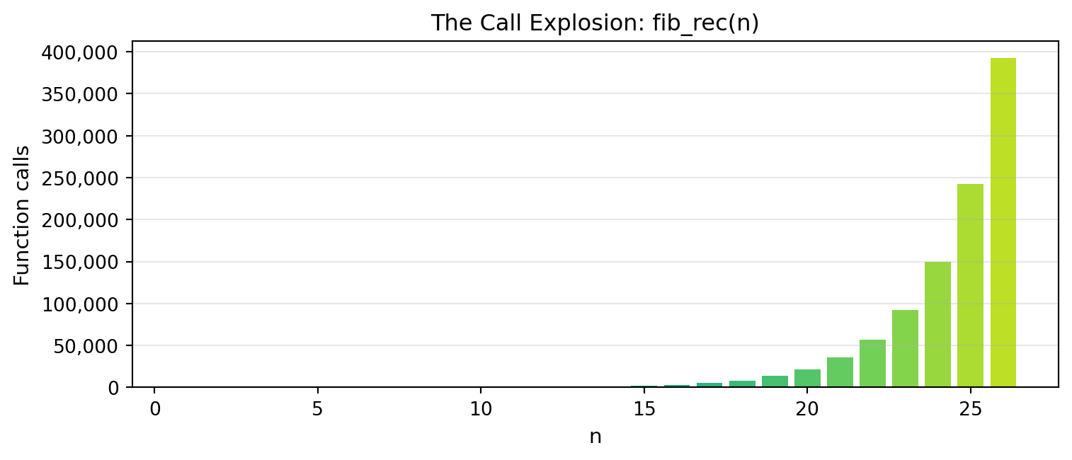
It works. But here is the trap: calling `fib_rec(35)` will recalculate
$F(34)$ once, $F(33)$ twice, $F(32)$ four times — every sub-problem
recomputed from scratch. The call count explodes exponentially.
### Research Example: How Fast Does Naive Recursion Blow Up? {.unnumbered .unlisted}
How fast does the call count grow with n — linearly, quadratically, or far worse?
```{=latex}
\needspace{18\baselineskip}
```
```{python}
#| label: fig-fib-call-explosion
#| fig-cap: "Naive recursion doubles its workload roughly every step. By n = 26, computing one Fibonacci number costs over 200,000 function calls."
import numpy as np
import matplotlib.pyplot as plt
import matplotlib.ticker as mticker

def count_calls(n):
    total = [0]
    def _f(k):
        total[0] += 1
        if k <= 1: return k
        return _f(k-1) + _f(k-2)
    _f(n)
    return total[0]

ns = list(range(1, 27))
calls = [count_calls(n) for n in ns]

fig, ax = plt.subplots(figsize=(8, 3.5))
colors = plt.get_cmap('viridis')(np.linspace(0.2, 0.9, len(ns)))
ax.bar(ns, calls, color=colors, edgecolor='none')
ax.set_xlabel('n', fontsize=11)
ax.set_ylabel('Function calls', fontsize=11)
ax.set_title('The Call Explosion: fib_rec(n)', fontsize=12)
ax.yaxis.set_major_formatter(mticker.FuncFormatter(lambda x, _: f'{int(x):,}'))
ax.grid(axis='y', alpha=0.3)
plt.tight_layout()
plt.show()
```
A bar that doubles with every step — that's the exponential tax on forgetting. A single call to `lru_cache` wipes out the entire bill.
**One line cures the explosion.** Python's `@lru_cache` stores every
result the first time it is computed — a stored answer is returned
instantly:
```{python}
from functools import lru_cache

@lru_cache(maxsize=None)
def fib_cached(n):
    if n <= 1:
        return n
    return fib_cached(n - 1) + fib_cached(n - 2)

print(f"F(100) cached = {fib_cached(100)}")
```
Each Fibonacci value is now computed exactly once, cutting the total
work from exponential back to $O(n)$.
<!-- TODO companion-02: Full analysis of fib_rec call count growth, proof that calls(n) = 2*F(n)-1, and the general principle of memoization / dynamic programming as technique -->
## Matrix Magic: Computing $F(n)$ in $O(\log n)$ Steps {#sec-fib-matrix}
There is a third algorithm that runs in $O(\log n)$ operations — not
$O(n)$, but the *logarithm* of $n$. The secret is a $2 \times 2$
matrix:
$$Q = \begin{pmatrix} 1 & 1 \\ 1 & 0 \end{pmatrix}, \quad
Q^n = \begin{pmatrix} F(n+1) & F(n) \\ F(n) & F(n-1) \end{pmatrix}.$$
Instead of multiplying $Q$ together $n$ times, Python computes $Q^2$,
then $(Q^2)^2 = Q^4$, then $Q^8$ — the answer in only
$\lceil \log_2 n \rceil$ multiplications. SymPy handles this
automatically with `**`:
```{python}
from sympy import Matrix

Q = Matrix([[1, 1], [1, 0]])

def fib_matrix(n):
    return int((Q**n)[0, 1])

all_match = all(fib_matrix(k) == fib_iter(k) for k in range(30))
print(f"Matrix matches iterative for k=0..29: {all_match}")
print(f"F(1000) ends in: ...{fib_matrix(1000) % 10**6}")
```
This matters when you need a single isolated value — $F(10^6)$, say —
without computing every number up to it.
<!-- TODO companion-02: Full derivation of Q^n = [[F(n+1), F(n)], [F(n), F(n-1)]] by induction; O(log n) repeated-squaring derivation; connection to Cayley-Hamilton theorem -->
## Identities: Every Formula Is a Hidden Treasure {#sec-fib-identities}
```{python}
#| echo: false
from pathlib import Path; import urllib.request
_d = Path('images'); _d.mkdir(exist_ok=True)
_p = _d / 'cassini.jpg'
if not _p.exists():
try:
req = urllib.request.Request(
'https://upload.wikimedia.org/wikipedia/commons/e/e5/Giovanni_Domenico_Cassini%2C_Biblioteca_Aprosiana.jpg',
headers={'User-Agent': 'Mozilla/5.0 (book project; educational use)'})
with urllib.request.urlopen(req) as r, open(_p, 'wb') as f:
f.write(r.read())
except Exception:
pass
```
::: {.content-visible when-format="pdf"}
```{=latex}
\begin{center}
\begin{minipage}[c]{0.22\textwidth}
\includegraphics[width=\textwidth]{images/cassini.jpg}
\end{minipage}%
\hspace{0.03\textwidth}%
\begin{minipage}[c]{0.55\textwidth}
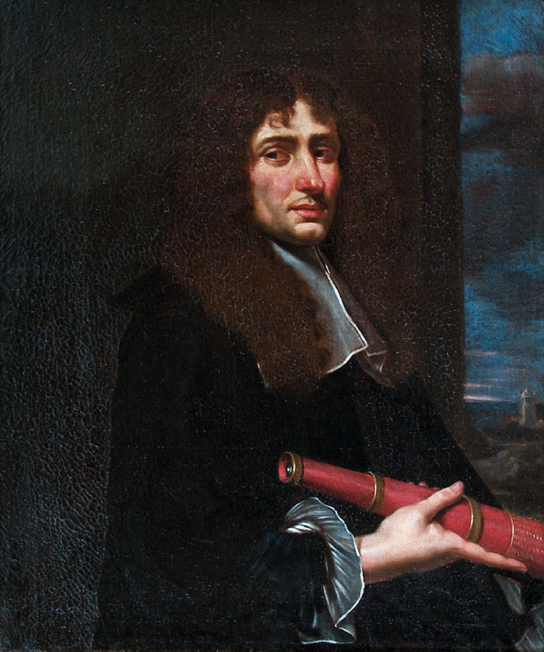
\small\textit{Giovanni Domenico Cassini (1625--1712)}\\[2pt]
\tiny Public domain, Biblioteca Aprosiana, via Wikimedia Commons
\end{minipage}
\end{center}
```
:::
::: {.content-visible when-format="html"}
<div style="display:flex; align-items:center; margin:1em 0; gap:12px;">
<img src="images/cassini.jpg" style="width:100px; flex-shrink:0;" alt="Giovanni Cassini">
<div style="font-size:0.82em;"><em>Giovanni Domenico Cassini (1625–1712)</em><br><span style="font-size:0.85em;">Public domain, Biblioteca Aprosiana, via Wikimedia Commons</span></div>
</div>
:::
The Fibonacci sequence satisfies dozens of algebraic identities — each
one waiting for you to *discover* it by experiment before you prove it.
**Cassini's identity.** An astronomer, not a mathematician, spotted
this gem in 1680. Compute $F(n-1) \cdot F(n+1) - F(n)^2$ and watch
what happens:
```{python}
# uses: fib_iter()
for n in range(2, 12):
    val = fib_iter(n-1) * fib_iter(n+1) - fib_iter(n)**2
    print(f"n={n:2d}: {val:3d}")
```
The result snaps between $-1$ and $+1$ forever:
$$F(n-1) \cdot F(n+1) - F(n)^2 = (-1)^n.$$
Why? Because the left side is $\det(Q^n) = (\det Q)^n = (-1)^n$. One
matrix identity, one proof.
**Sum of consecutive Fibonacci numbers.** Add up the first $n$ terms:
```{python}
# uses: fib_iter()
for n in range(1, 10):
    total = sum(fib_iter(k) for k in range(1, n+1))
    print(f"sum F(1..{n}) = {total},  F({n+2})-1 = {fib_iter(n+2)-1}")
```
Always $F(n+2) - 1$. The pattern:
$\sum_{k=1}^{n} F(k) = F(n+2) - 1.$
**Addition formula.** For any indices $m$ and $n$:
$$F(m+n) = F(m) \cdot F(n+1) + F(m-1) \cdot F(n).$$
```{python}
# uses: fib_iter()
errors = 0
for m in range(1, 15):
    for n in range(1, 15):
        lhs = fib_iter(m + n)
        rhs = fib_iter(m) * fib_iter(n+1) + fib_iter(m-1) * fib_iter(n)
        if lhs != rhs:
            errors += 1
print(f"Addition formula errors in 1..14 × 1..14: {errors}")
```
**The GCD identity — arguably the most stunning of all:**
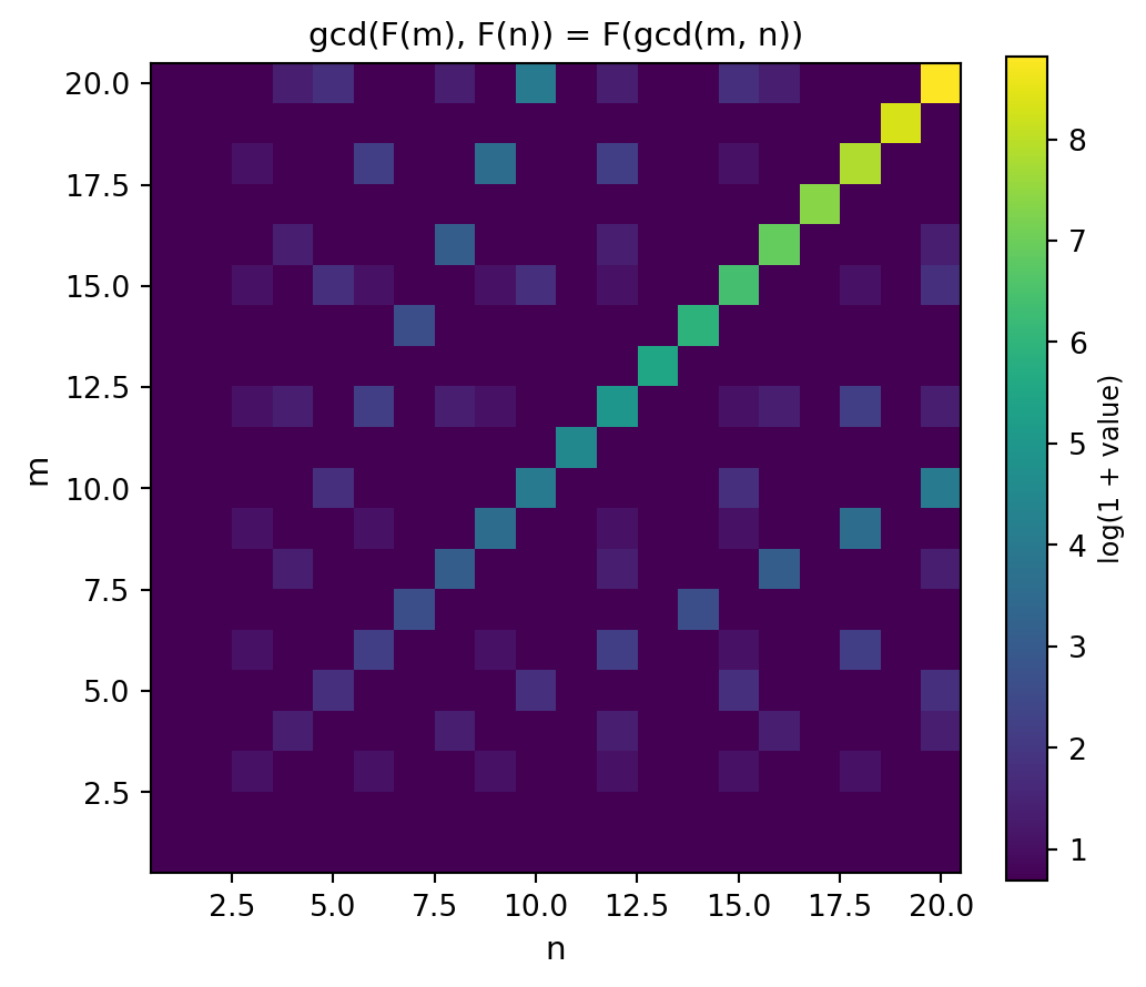
$$\gcd(F(m),\, F(n)) = F(\gcd(m,\, n)).$$
Two Fibonacci numbers share a common factor *if and only if* their
positions share a common factor. The index carries the divisibility:
```{python}
# uses: fib_iter()
from math import gcd

for m in [12, 15, 20, 24]:
    for n in [8, 10, 18]:
        lhs = gcd(fib_iter(m), fib_iter(n))
        rhs = fib_iter(gcd(m, n))
        ok = lhs == rhs
        print(f"gcd(F({m}),F({n}))={lhs}  F(gcd({m},{n}))={rhs}  {ok}")
```
### Research Example: Does the GCD Identity Paint a Pattern? {.unnumbered .unlisted}
Compute $F(\gcd(m, n))$ for every pair in a 20×20 grid — does a structured picture emerge, or just noise?
```{=latex}
\needspace{20\baselineskip}
```
```{python}
#| label: fig-fib-gcd-grid
#| fig-cap: "Each cell shows F(gcd(m, n)). Bands of color reveal the divisibility structure of the Fibonacci sequence — stripes appear wherever two indices share a factor."
import numpy as np
import matplotlib.pyplot as plt
from math import gcd

def fib_iter(n):
    a, b = 0, 1
    for _ in range(n):
        a, b = b, a + b
    return a


M = 20
grid = np.array([[fib_iter(gcd(m, n)) for n in range(1, M+1)]
                  for m in range(1, M+1)], dtype=float)

fig, ax = plt.subplots(figsize=(5.5, 5))
im = ax.imshow(np.log1p(grid), cmap='viridis', origin='lower',
               extent=[0.5, M+0.5, 0.5, M+0.5])
ax.set_xlabel('n', fontsize=11)
ax.set_ylabel('m', fontsize=11)
ax.set_title('gcd(F(m), F(n)) = F(gcd(m, n))', fontsize=11)
cbar = fig.colorbar(im, ax=ax, fraction=0.046)
cbar.set_label('log(1 + value)', fontsize=9)
plt.tight_layout()
plt.show()
```
The diagonal stripes are divisibility in disguise. Any index that shares a factor with another produces a brighter cell — and the whole structure emerges from a single six-word identity. You wrote the code; the pattern wrote itself.
## Every Number Has a Fibonacci Fingerprint {#sec-fib-zeckendorf}
Here is a claim that sounds impossible: **every positive integer can be
written as a sum of distinct, non-consecutive Fibonacci numbers in
exactly one way.** This is **Zeckendorf's theorem** [@zeckendorf1972], proved in 1972.
For example, $20 = 13 + 5 + 2$. Check: 13, 5, and 2 are all
Fibonacci numbers, all distinct, and no two are consecutive ($F(7)=13$,
$F(5)=5$ — there is a gap). No other such representation of 20 exists.
The **greedy algorithm** finds the representation instantly: subtract
the largest Fibonacci number that fits, repeat:
```{python}
def zeckendorf(n):
    fs = [1, 2]
    while fs[-1] < n:
        fs.append(fs[-1] + fs[-2])
    parts = []
    remaining = n
    for f in reversed(fs):
        if f <= remaining:
            parts.append(f)
            remaining -= f
    return parts

for n in range(1, 21):
    z = zeckendorf(n)
    parts_str = " + ".join(str(f) for f in z)
    print(f"{n:3d} = {parts_str}")
```
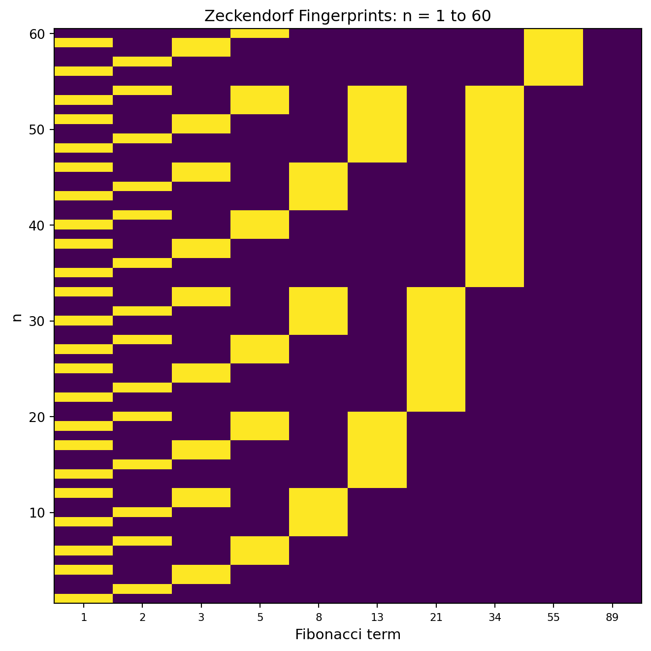
### Research Example: What Does Every Number's Fibonacci Fingerprint Look Like? {.unnumbered .unlisted}
Paint the Zeckendorf representation of every number from 1 to 60 as a barcode — does any rule show up visually?
```{=latex}
\needspace{22\baselineskip}
```
```{python}
#| label: fig-fib-zeckendorf-barcode
#| fig-cap: "Each row is a number 1–60; each column is a Fibonacci term. A bright cell means that term appears in the Zeckendorf representation. Notice no two adjacent columns are ever both lit in the same row."
import numpy as np
import matplotlib.pyplot as plt

def zeckendorf(n):
    fs = [1, 2]
    while fs[-1] < n:
        fs.append(fs[-1] + fs[-2])
    parts = []
    remaining = n
    for f in reversed(fs):
        if f <= remaining:
            parts.append(f)
            remaining -= f
    return parts


fibs = [1, 2, 3, 5, 8, 13, 21, 34, 55, 89]
N = 60
barcode = np.zeros((N, len(fibs)))
for n in range(1, N + 1):
    z = set(zeckendorf(n))
    for j, f in enumerate(fibs):
        if f in z:
            barcode[n-1, j] = 1

fig, ax = plt.subplots(figsize=(7, 7))
ax.imshow(barcode, aspect='auto', cmap='viridis', origin='lower',
          extent=[0.5, len(fibs)+0.5, 0.5, N+0.5])
ax.set_xticks(range(1, len(fibs)+1))
ax.set_xticklabels([str(f) for f in fibs], fontsize=8)
ax.set_xlabel('Fibonacci term', fontsize=11)
ax.set_ylabel('n', fontsize=11)
ax.set_title('Zeckendorf Fingerprints: n = 1 to 60', fontsize=12)
plt.tight_layout()
plt.show()
```
Scan the barcode: columns 55 and 89 (adjacent Fibonacci numbers) are never both bright in the same row. Zeckendorf's theorem is encoded in the visual structure itself.
You just ran an experiment that would have taken a mathematician years of pen-and-paper work. The theorem was proved in 1972 — your code reproduced its core evidence in seconds.
<!-- TODO companion-03: Full proof of Zeckendorf's theorem by strong induction — existence via greedy algorithm, uniqueness via no-consecutive-Fibonacci constraint -->
## The Secret Life of the Last Digits {#sec-fib-pisano}
::: {.content-visible when-format="pdf"}
```{=latex}
\begin{center}
\begin{minipage}[c]{0.28\textwidth}
\centering
\href{https://youtu.be/o1eLKODSCqw}{\includegraphics[width=\textwidth]{images/thumb_o1eLKODSCqw.jpg}}
\end{minipage}%
\hspace{0.02\textwidth}%
\begin{minipage}[c]{0.28\textwidth}
\small\textbf{Jacob Yatsko}\\[3pt]
\small A New Way to Look at Fibonacci Numbers\\[3pt]
\small\href{https://youtu.be/o1eLKODSCqw}{\texttt{youtu.be/o1eLKODSCqw}}
\end{minipage}%
\hspace{0.02\textwidth}%
\begin{minipage}[c]{0.36\textwidth}
\small Reframes Fibonacci numbers as a tiling problem, showing how counting ways to fill a strip with 1×1 and 1×2 tiles produces the sequence naturally.
\end{minipage}
\end{center}
```
:::
::: {.content-visible when-format="html"}
<div style="display:flex; align-items:flex-start; margin:1em 0; gap:12px; width:100%;">
<div style="flex:0 0 200px;"><a href="https://youtu.be/o1eLKODSCqw" target="_blank"><img src="https://img.youtube.com/vi/o1eLKODSCqw/0.jpg" style="width:100%;display:block;" alt="A New Way to Look at Fibonacci Numbers"></a></div>
<div style="flex:1; font-size:0.85em;"><strong>Jacob Yatsko</strong><br>A New Way to Look at Fibonacci Numbers<br><a href="https://youtu.be/o1eLKODSCqw" target="_blank" style="font-family:Consolas,monospace;">youtu.be/o1eLKODSCqw</a></div>
<div style="flex:1; font-size:0.85em;">Reframes Fibonacci numbers as a tiling problem, showing how counting ways to fill a strip with 1×1 and 1×2 tiles produces the sequence naturally.</div>
</div>
:::
What do the *last digits* of Fibonacci numbers look like? Print the
first 25 values modulo 10 and watch for a repeat:
```{python}
# uses: fib_iter()
import pprint
fibs_mod10 = [fib_iter(k) % 10 for k in range(25)]
print("F(n) mod 10, n=0..24:")
# width=60 wraps long output to fit the printed page
pprint.pprint(fibs_mod10, width=60, compact=True)
```
The last digit of Fibonacci numbers repeats with period **60**. For
any modulus $m$, the sequence $F(0) \bmod m,\ F(1) \bmod m, \ldots$
is eventually periodic and always returns to $(0, 1)$. The length of
this cycle is the **Pisano period** $\pi(m)$:
```{python}
def pisano_period(m):
    a, b = 0, 1
    for i in range(1, 6 * m + 2):
        a, b = b, (a + b) % m
        if a == 0 and b == 1:
            return i
    return -1

print(f"{'m':>4}  {'pi(m)':>7}")
print("-" * 14)
for m in range(2, 21):
    print(f"{m:>4}  {pisano_period(m):>7}")
```
The pattern of Pisano periods contains its own mysteries — powers of
10, sudden jumps, and deep connections to prime structure.
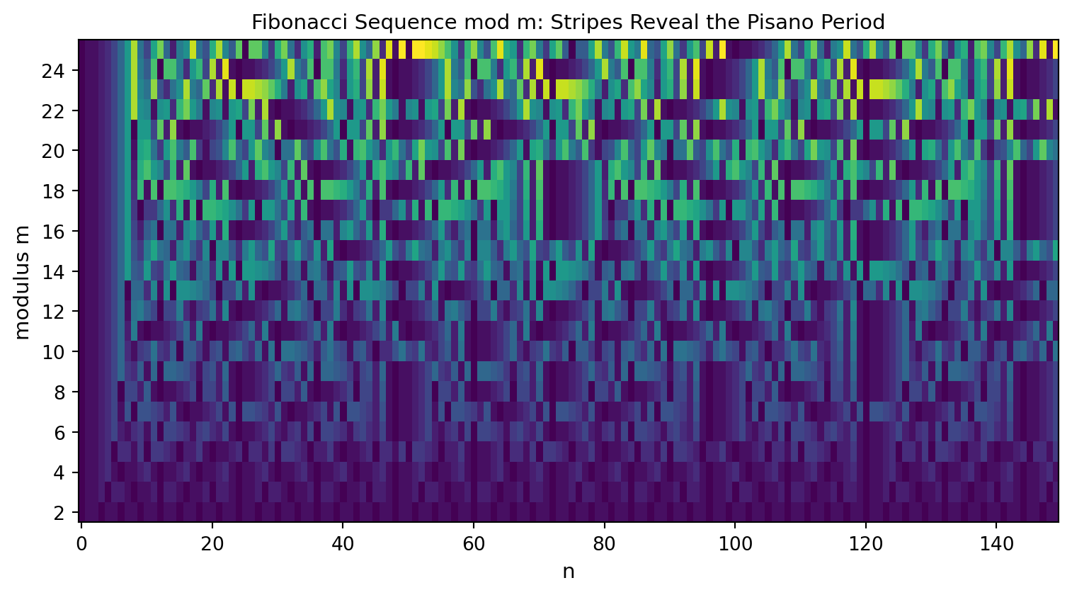
### Research Example: Can We See All Pisano Periods at Once? {.unnumbered .unlisted}
Display $F(n) \bmod m$ for every modulus $m$ from 2 to 25 in a single image — do the repeating cycles become visible?
```{=latex}
\needspace{22\baselineskip}
```
```{python}
#| label: fig-pisano-heatmap
#| fig-cap: "Each row shows F(n) mod m for one modulus m (2 to 25). The stripes reveal the Pisano period — where the colors repeat, the cycle restarts. Modulus 10 (row 9) has period 60."
import numpy as np
import matplotlib.pyplot as plt

def fib_iter(n):
    a, b = 0, 1
    for _ in range(n):
        a, b = b, a + b
    return a


rows = 24
cols = 150
pisano_grid = np.array(
    [[fib_iter(n) % m for n in range(cols)]
     for m in range(2, rows + 2)], dtype=float)

fig, ax = plt.subplots(figsize=(8, 4.5))
ax.imshow(pisano_grid, aspect='auto', cmap='viridis', origin='lower',
          extent=[-0.5, cols-0.5, 1.5, rows+1.5])
ax.set_xlabel('n', fontsize=11)
ax.set_ylabel('modulus m', fontsize=11)
ax.set_title('Fibonacci Sequence mod m: Stripes Reveal the Pisano Period',
             fontsize=11)
ax.set_yticks(range(2, rows + 2, 2))
plt.tight_layout()
plt.show()
```
Every stripe you see is a hidden clock — and you mapped twenty-four of them simultaneously. Any one of those rows would have been a publishable observation before computers existed.
## Fibonacci's Closest Cousin: The Lucas Numbers {#sec-fib-lucas}
::: {.content-visible when-format="pdf"}
```{=latex}
\begin{center}
\begin{minipage}[c]{0.28\textwidth}
\centering
\href{https://youtu.be/PeUbRXnbmms}{\includegraphics[width=\textwidth]{images/thumb_PeUbRXnbmms.jpg}}
\end{minipage}%
\hspace{0.02\textwidth}%
\begin{minipage}[c]{0.28\textwidth}
\small\textbf{Numberphile}\\[3pt]
\small Lucas Numbers\\[3pt]
\small\href{https://youtu.be/PeUbRXnbmms}{\texttt{youtu.be/PeUbRXnbmms}}
\end{minipage}%
\hspace{0.02\textwidth}%
\begin{minipage}[c]{0.36\textwidth}
\small Explores the Lucas sequence — same recurrence as Fibonacci but starting 2, 1 — and shows how it interleaves with Fibonacci through surprising identities.
\end{minipage}
\end{center}
```
:::
::: {.content-visible when-format="html"}
<div style="display:flex; align-items:flex-start; margin:1em 0; gap:12px; width:100%;">
<div style="flex:0 0 200px;"><a href="https://youtu.be/PeUbRXnbmms" target="_blank"><img src="https://img.youtube.com/vi/PeUbRXnbmms/0.jpg" style="width:100%;display:block;" alt="Lucas Numbers"></a></div>
<div style="flex:1; font-size:0.85em;"><strong>Numberphile</strong><br>Lucas Numbers<br><a href="https://youtu.be/PeUbRXnbmms" target="_blank" style="font-family:Consolas,monospace;">youtu.be/PeUbRXnbmms</a></div>
<div style="flex:1; font-size:0.85em;">Explores the Lucas sequence — same recurrence as Fibonacci but starting 2, 1 — and shows how it interleaves with Fibonacci through surprising identities.</div>
</div>
:::
```{python}
#| echo: false
from pathlib import Path; import urllib.request
_d = Path('images'); _d.mkdir(exist_ok=True)
_p = _d / 'edouard_lucas.png'
if not _p.exists():
try:
_req = urllib.request.Request('https://upload.wikimedia.org/wikipedia/commons/a/ad/Elucas_1.png', headers={'User-Agent': 'Mozilla/5.0 (educational-book-project)'})
with urllib.request.urlopen(_req) as _resp: _p.write_bytes(_resp.read())
except Exception: pass
```
::: {.content-visible when-format="pdf"}
```{=latex}
\begin{center}
\begin{minipage}[c]{0.22\textwidth}
\includegraphics[width=\textwidth]{images/edouard_lucas.png}
\end{minipage}%
\hspace{0.03\textwidth}%
\begin{minipage}[c]{0.55\textwidth}
\small\textit{Édouard Lucas (1842--1891)}\\[2pt]
\tiny Public domain, via Wikimedia Commons
\end{minipage}
\end{center}
```
:::
::: {.content-visible when-format="html"}
<div style="display:flex; align-items:center; margin:1em 0; gap:12px;">
<img src="images/edouard_lucas.png" style="width:100px; flex-shrink:0;" alt="Édouard Lucas">
<div style="font-size:0.82em;"><em>Édouard Lucas (1842–1891)</em><br><span style="font-size:0.85em;">Public domain, via Wikimedia Commons</span></div>
</div>
:::
Change the starting values from $(F(0), F(1)) = (0, 1)$ to
$(L(0), L(1)) = (2, 1)$ and apply the same recurrence. The result is
the **Lucas sequence**, named after Édouard Lucas (1842–1891), the
French mathematician who first studied Fibonacci numbers systematically:
$$2,\; 1,\; 3,\; 4,\; 7,\; 11,\; 18,\; 29,\; 47,\; 76, \ldots$$
```{python}
import pprint

def lucas(n):
    a, b = 2, 1
    for _ in range(n):
        a, b = b, a + b
    return a

lucas20 = [lucas(k) for k in range(20)]
print("L(0) through L(19):")
# width=60 wraps long output to fit the printed page
pprint.pprint(lucas20, width=60, compact=True)
```
The deep connection to Fibonacci: every Lucas number is the sum of two
Fibonacci numbers one step apart.
```{python}
# uses: lucas(), fib_iter()
print(f"{'n':>4}  {'L(n)':>8}  {'F(n-1)+F(n+1)':>15}  match")
for n in range(1, 12):
    lhs = lucas(n)
    rhs = fib_iter(n-1) + fib_iter(n+1)
    print(f"{n:>4}  {lhs:>8}  {rhs:>15}  {lhs==rhs}")
```
$$L(n) = F(n-1) + F(n+1).$$
Lucas numbers also have their own Pisano-style periods, their own
Cassini-like identity ($L(n-1) \cdot L(n+1) - L(n)^2 = 5 \cdot (-1)^n$),
and a Binet-style closed form. They are not a curiosity — Lucas used
them to prove that $2^{127} - 1$ is prime, a record that stood for
75 years.
## The Number That Conquered Nature {#sec-fib-golden}
```{python}
#| echo: false
_d = Path('images'); _d.mkdir(exist_ok=True)
_p = _d / 'binet.jpg'
if not _p.exists():
try:
req = urllib.request.Request(
'https://upload.wikimedia.org/wikipedia/commons/a/af/Jacques_Binet.jpg',
headers={'User-Agent': 'Mozilla/5.0 (book project; educational use)'})
with urllib.request.urlopen(req) as r, open(_p, 'wb') as f:
f.write(r.read())
except Exception:
pass
```
::: {.content-visible when-format="pdf"}
```{=latex}
\begin{center}
\begin{minipage}[c]{0.22\textwidth}
\includegraphics[width=\textwidth]{images/binet.jpg}
\end{minipage}%
\hspace{0.03\textwidth}%
\begin{minipage}[c]{0.55\textwidth}
\small\textit{Jacques-Philippe-Marie Binet (1786--1856)}\\[2pt]
\tiny Public domain, via Wikimedia Commons
\end{minipage}
\end{center}
```
:::
::: {.content-visible when-format="html"}
<div style="display:flex; align-items:center; margin:1em 0; gap:12px;">
<img src="images/binet.jpg" style="width:100px; flex-shrink:0;" alt="Jacques Binet">
<div style="font-size:0.82em;"><em>Jacques-Philippe-Marie Binet (1786–1856)</em><br><span style="font-size:0.85em;">Public domain, via Wikimedia Commons</span></div>
</div>
:::
Watch consecutive ratios $F(n+1)/F(n)$ as $n$ grows:
```{python}
# uses: fib_iter()
print(f"{'n':>4}  {'F(n+1)/F(n)':>18}")
print("-" * 25)
for n in range(1, 16):
    ratio = fib_iter(n+1) / fib_iter(n)
    print(f"{n:>4}  {ratio:>18.10f}")
```
They converge to the **golden ratio**
$\phi = (1 + \sqrt{5})/2 \approx 1.61803\ldots$ — the positive
solution to $L = 1 + 1/L$.
**Binet's formula** gives $F(n)$ without any iteration at all:
$$F(n) = \frac{\phi^n - \psi^n}{\sqrt{5}}, \quad
\psi = \frac{1 - \sqrt{5}}{2} \approx -0.618.$$
Because $|\psi| < 1$, its contribution is always less than $\tfrac{1}{2}$,
so $F(n)$ is simply $\phi^n / \sqrt{5}$ rounded to the nearest integer.
```{python}
# uses: fib_iter()
import math

phi = (1 + math.sqrt(5)) / 2
psi = (1 - math.sqrt(5)) / 2

print(f"{'n':>3}  {'Binet':>10}  {'fib_iter':>10}  match")
print("-" * 42)
for n in range(10):
    binet = (phi**n - psi**n) / math.sqrt(5)
    exact = fib_iter(n)
    print(f"{n:>3}  {binet:>10.4f}  {exact:>10}  {round(binet) == exact}")
```
```{=latex}
\needspace{28\baselineskip}
```
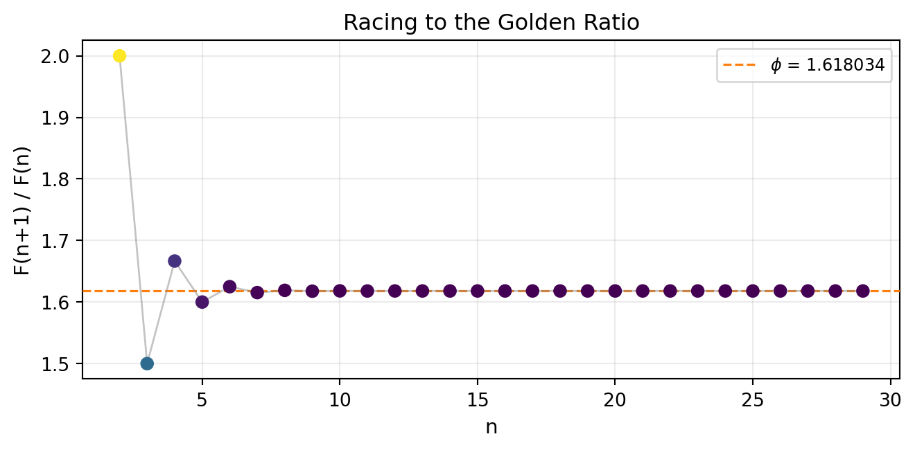
### Research Example: How Quickly Does F(n+1)/F(n) Lock Onto the Golden Ratio? {.unnumbered .unlisted}
Plot each ratio $F(n+1)/F(n)$ for $n = 2$ to 29, coloring each point by its remaining distance from $\phi$ — does the approach look sudden or gradual?
```{python}
#| label: fig-fib-convergence
#| fig-cap: "Ratios F(n+1)/F(n) lock onto the golden ratio phi = 1.61803... The colors show the distance from phi — bright for far, dark for close."
import numpy as np
import matplotlib.pyplot as plt
import math

ORANGE = '#ff7f0e'

def fib_iter(n):
    a, b = 0, 1
    for _ in range(n):
        a, b = b, a + b
    return a


phi = (1 + math.sqrt(5)) / 2
ns_conv = list(range(2, 30))
ratios = [fib_iter(n+1) / fib_iter(n) for n in ns_conv]
errors_conv = [abs(r - phi) for r in ratios]

fig, ax = plt.subplots(figsize=(7, 3.5))
sc = ax.scatter(ns_conv, ratios,
                c=np.log1p(errors_conv), cmap='viridis',
                s=40, zorder=5)
ax.plot(ns_conv, ratios, '-', color='#888888', alpha=0.5,
        linewidth=1, zorder=4)
ax.axhline(phi, color=ORANGE, linestyle='--', linewidth=1.2,
           label=f'$\\phi$ = {phi:.6f}', zorder=3)
ax.set_xlabel('n', fontsize=11)
ax.set_ylabel('F(n+1) / F(n)', fontsize=11)
ax.set_title('Racing to the Golden Ratio', fontsize=12)
ax.legend(fontsize=9)
ax.grid(alpha=0.25)
plt.tight_layout()
plt.show()
```
By $n = 15$ the ratio is already correct to six decimal places. The colors make the remaining error visible long after the numbers themselves look identical. You spotted the exponential approach to $\phi$ — the same pattern that makes Binet's formula work.
**Nature's secret reason for $\phi$.** Sunflowers pack seeds in two
spiraling families, with consecutive Fibonacci numbers of spirals in
each direction (34 and 55, or 55 and 89). The reason is that $\phi$ is
the "most irrational" number — its continued fraction is
$[1; 1, 1, 1, \ldots]$, the hardest number to approximate by a
fraction. Seeds placed at angle $2\pi/\phi^2$ apart spread as uniformly
as possible:
::: {.content-visible when-format="pdf"}
```{=latex}
\begin{center}
\begin{minipage}[c]{0.28\textwidth}
\centering
\href{https://youtu.be/kkGeOWYOFoA}{\includegraphics[width=\textwidth]{images/thumb_kkGeOWYOFoA.jpg}}
\end{minipage}%
\hspace{0.02\textwidth}%
\begin{minipage}[c]{0.28\textwidth}
\small\textbf{Crist\'obal Vila / Et\'erea Estudios}\\[3pt]
\small Nature by Numbers\\[3pt]
\small\href{https://youtu.be/kkGeOWYOFoA}{\texttt{youtu.be/kkGeOWYOFoA}}
\end{minipage}%
\hspace{0.02\textwidth}%
\begin{minipage}[c]{0.36\textwidth}
\small A stunning short film that animates how Fibonacci numbers, the golden ratio, and spiral geometry appear in sunflowers, shells, and dragonfly wings.
\end{minipage}
\end{center}
```
:::
::: {.content-visible when-format="html"}
<div style="display:flex; align-items:flex-start; margin:1em 0; gap:12px; width:100%;">
<div style="flex:0 0 200px;"><a href="https://youtu.be/kkGeOWYOFoA" target="_blank"><img src="https://img.youtube.com/vi/kkGeOWYOFoA/0.jpg" style="width:100%;display:block;" alt="Nature by Numbers"></a></div>
<div style="flex:1; font-size:0.85em;"><strong>Cristóbal Vila / Etérea Estudios</strong><br>Nature by Numbers<br><a href="https://youtu.be/kkGeOWYOFoA" target="_blank" style="font-family:Consolas,monospace;">youtu.be/kkGeOWYOFoA</a></div>
<div style="flex:1; font-size:0.85em;">A stunning short film that animates how Fibonacci numbers, the golden ratio, and spiral geometry appear in sunflowers, shells, and dragonfly wings.</div>
</div>
:::
### Research Example: Does the Golden Angle Actually Produce Fibonacci Spirals? {.unnumbered .unlisted}
Place 600 seeds at consecutive golden-angle steps and plot the result — do Fibonacci spiral counts appear spontaneously?
```{=latex}
\needspace{22\baselineskip}
```
```{python}
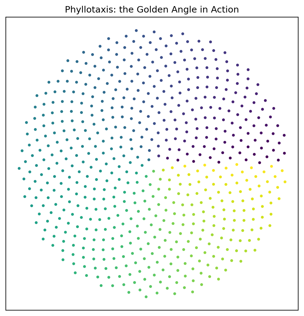
#| label: fig-fib-sunflower
#| fig-cap: "600 seeds placed at consecutive golden-angle steps. The eye sees spirals — 21 and 34, or 34 and 55 — counting Fibonacci numbers each time."
import numpy as np
import matplotlib.pyplot as plt
import math

phi = (1 + math.sqrt(5)) / 2

N_seeds = 600
k_seeds = np.arange(1, N_seeds + 1)
golden_angle = 2 * np.pi / phi**2
theta_seeds = k_seeds * golden_angle
r_seeds = np.sqrt(k_seeds)
x_seeds = r_seeds * np.cos(theta_seeds)
y_seeds = r_seeds * np.sin(theta_seeds)

fig, ax = plt.subplots(figsize=(5.5, 5.5))
colors = plt.get_cmap('viridis')(theta_seeds / (2 * np.pi) % 1.0)
ax.scatter(x_seeds, y_seeds, s=12, c=colors, linewidths=0)
ax.set_aspect('equal')
ax.set_xticks([])
ax.set_yticks([])
ax.set_title('Phyllotaxis: the Golden Angle in Action', fontsize=11)
plt.tight_layout()
plt.show()
```
Count the spirals going clockwise, then counterclockwise: you will find two consecutive Fibonacci numbers. Change the angle by even a fraction of a percent and the spirals disappear into chaos.
Thirty lines of code reproduced a pattern evolution needed 400 million years to discover. That's the power you now hold.
<!-- TODO companion-03: Proof that phi = [1;1,1,1,...] is the "most irrational" number via Hurwitz's theorem on rational approximation -->
## Further Research Topics {#sec-fib-research}
The following problems range from short experiments to semester-length
projects. They are listed from easiest to most open-ended.
1. **Last-digit period.** Verify by hand (using paper and pencil, not
code) that the Fibonacci sequence modulo 10 has period 60. Then
write code to find all Pisano periods up to $m = 100$ and look for
patterns. Which values of $m$ give the smallest period relative to
$m$? Which give the largest?
*(Problem proposed by Claude Code.)*
2. **Cassini's identity for Lucas numbers.** The Lucas numbers satisfy
the same recurrence as Fibonacci but start with $L(0) = 2$ and
$L(1) = 1$. Compute the analogous product $L(n-1) \cdot L(n+1) -
L(n)^2$ for $n = 2, 3, \ldots, 15$. State a conjecture and verify
it symbolically using the matrix approach.
*(Problem proposed by Claude Code.)*
3. **Sum of even-indexed Fibonacci numbers.** Compute
$\sum_{k=1}^{n} F(2k)$ for $n = 1, 2, \ldots, 10$. Compare each
sum to Fibonacci numbers. Find a closed-form conjecture and prove
it using the sum formula from @sec-fib-identities.
*(Problem proposed by Claude Code.)*
4. **Fibonacci primes.** By the GCD identity from @sec-fib-identities,
$F(n)$ can be prime only when $n$ is prime (or $n = 4$). Check
which prime indices $p \leq 100$ give a prime $F(p)$. How rare are
Fibonacci primes? Extend the search to $p \leq 1000$ using SymPy's
`isprime` (introduced in @sec-primes-what).
*(Problem proposed by Claude Code.)*
5. **Wall's conjecture (open problem).** Define a prime $p$ to be a
**Wall-Sun-Sun prime** if $F(p) \equiv 0 \pmod{p^2}$. No such
prime is known. Search for Wall-Sun-Sun primes among the first 1000
primes. How close does each prime come? Plot the residue
$F(p) \bmod p^2$ versus $p$.
*(Problem proposed by Claude Code.)*
6. **Zeckendorf digit sums.** For each $n$ from 1 to 200, count how
many terms appear in its Zeckendorf representation (the number of
1s in the Fibonacci base representation). Plot the distribution.
What is the average number of terms? How does it grow with $n$?
*(Problem proposed by Claude Code.)*
7. **Fibonacci meets modular arithmetic.** Show experimentally that
$F(np) \equiv 0 \pmod{F(n)}$ for all positive integers $n$ and $p$.
(Hint: use the addition formula from @sec-fib-identities repeatedly.)
Then verify this for $n = 1, \ldots, 20$ and $p = 1, \ldots, 10$.
*(Problem proposed by Claude Code.)*
8. **Pisano periods for prime powers.** Let $p$ be a prime and
compute $\pi(p)$, $\pi(p^2)$, $\pi(p^3)$. Do you see a pattern?
Conjecture a formula for $\pi(p^k)$ in terms of $\pi(p)$ and test
it for $p \in \{2, 3, 5, 7, 11, 13\}$.
*(Problem proposed by Claude Code.)*
9. **Generalized Fibonacci sequences.** Choose two starting values
$a$ and $b$ and apply the Fibonacci recurrence $G(n) = G(n-1) +
G(n-2)$. Does the ratio $G(n+1)/G(n)$ still converge to $\phi$
regardless of $a$ and $b$ (as long as both are not zero)? Prove
your answer using Binet-style analysis.
*(Problem proposed by Claude Code.)*
10. **Fibonacci and Pascal's triangle.** Sum the entries of Pascal's
triangle along "shallow diagonals": $\binom{n}{0}$,
$\binom{n-1}{1}$, $\binom{n-2}{2}$, and so on. Compare these
diagonal sums to Fibonacci numbers. Prove the connection using
the binomial theorem or induction.
*(Problem proposed by Claude Code.)*
11. **Fibonacci in other bases.** The Fibonacci number system uses base
$(1, 2, 3, 5, 8, \ldots)$. Define addition in this system by
carrying according to the rules $2 \cdot F(k) = F(k+1) + F(k-2)$.
Implement Fibonacci-base addition and verify it produces correct
sums for all pairs up to 100. What makes this base useful for
certain computer architectures?
*(Problem proposed by Claude Code.)*
12. **Matrix method for other recurrences.** The matrix technique from
@sec-fib-matrix works for any linear recurrence. Consider the
Tribonacci sequence: $T(n) = T(n-1) + T(n-2) + T(n-3)$ with
$T(0) = 0$, $T(1) = 0$, $T(2) = 1$. Construct the $3 \times 3$
companion matrix, verify the identity $M^n_{0,1} = T(n)$, and
find the limiting ratio $T(n+1)/T(n)$ experimentally. What
polynomial does this limit satisfy?
*(Problem proposed by Claude Code.)*
13. **Golden ratio and continued fractions.** Express $\phi$ as an
infinite continued fraction by applying the algorithm from
Chapter 7 (once you reach it). You will find that $\phi = [1; 1,
1, 1, \ldots]$, the simplest possible pattern. Verify that the
convergents of this continued fraction are exactly consecutive
Fibonacci ratios $F(n+1)/F(n)$.
*(Problem proposed by Claude Code.)*
14. **Fibonacci spirals in nature.** Sunflowers display $F(n)$ and
$F(n+1)$ spirals in their seed heads (commonly 34 and 55, or 55
and 89). Write code that generates a point cloud mimicking a
sunflower by placing seed $k$ at polar coordinates
$(r, \theta) = (\sqrt{k},\ 2\pi k / \phi^2)$. Plot the result.
Vary the angle slightly (e.g., use $\pi$ instead of $2\pi/\phi^2$)
and compare. Why does $\phi$ produce the most uniform packing?
*(Problem proposed by Claude Code.)*
15. **Distribution of Fibonacci digits.** By Binet's formula, $F(n)$
has approximately $n \log_{10} \phi \approx 0.209n$ decimal digits.
Apply Benford's law [@benford1938]: compute the leading decimal digit of each of
the first 1000 Fibonacci numbers and plot the frequency distribution.
Compare to the Benford prediction $\log_{10}(1 + 1/d)$. Explain
theoretically why Fibonacci numbers follow Benford's law.
*(Problem proposed by Claude Code.)*
16. **Pythagorean triples from Fibonacci.** Take any four consecutive
Fibonacci numbers $F(n), F(n+1), F(n+2), F(n+3)$ and form the
triple
$$a = F(n) \cdot F(n+3), \quad b = 2 F(n+1) F(n+2), \quad
c = F(n+1)^2 + F(n+2)^2.$$
Verify that $a^2 + b^2 = c^2$ for $n = 1, 2, \ldots, 20$.
Then prove the identity algebraically: note that
$F(n+2) - F(n+1) = F(n)$ and $F(n+2) + F(n+1) = F(n+3)$, so
$c^2 - b^2 = (F(n+2)^2 - F(n+1)^2)^2 = (F(n) F(n+3))^2 = a^2$.
Which of these triples are primitive (i.e., $\gcd(a, b, c) = 1$)?
Characterize exactly which values of $n$ give a primitive triple.
*(Problem proposed by Claude Code.)*
17. **The Fibonacci word.** Define the substitution $0 \to 01$,
$1 \to 0$ and apply it repeatedly starting from $0$:
$$0,\; 01,\; 010,\; 01001,\; 01001010, \ldots$$
Generate the first 2000 characters of this infinite sequence.
Count the frequency of $0$s: what does the ratio
$\text{(number of 0s)}/\text{(length)}$ converge to? Explain the
connection to $1/\phi$. Then look for the pattern $00$ in the word:
prove it never occurs. (Hint: $F(n)$ consecutive 0s cannot appear
for $n \geq 2$.) How does the Fibonacci word relate to the automata
model in @sec-automata-intro?
*(Problem proposed by Claude Code.)*
18. **GCD identity and divisibility lattice.** One of the most elegant
Fibonacci theorems states
$$\gcd\!\bigl(F(m),\, F(n)\bigr) = F\!\bigl(\gcd(m, n)\bigr).$$
Verify this computationally for all pairs $1 \le m, n \le 60$.
Then prove it in two steps: (a) show that $F(n) \mid F(kn)$ for
all positive integers $k$ using the addition formula
$F(m+n) = F(m-1)F(n) + F(m)F(n+1)$ from @sec-fib-identities;
(b) imitate the Euclidean algorithm on the indices to reduce
$\gcd(F(m), F(n))$ to $F(\gcd(m,n))$. Use this identity to
re-examine Fibonacci primes from topic 4: if $F(n)$ is prime and
$n$ is composite, what does the GCD identity force?
*(Problem proposed by Claude Code.)*
19. **The concatenated Fibonacci constant.** Form the real number
$$\mathcal{F} = 0.\underbrace{1\,1\,2\,3\,5\,8\,1\,3\,2\,1\,3\,4\,5\,5\ldots}_{\text{Fibonacci numbers written in order}}$$
by concatenating the decimal representations of
$F(1), F(2), F(3), \ldots$ [@martin2011, p. 637].
Write code to generate the first 10\,000 digits of $\mathcal{F}$.
Apply the frequency test: does each digit $0$–$9$ appear with
frequency close to $1/10$? Apply the block test for pairs and
triples of consecutive digits. Based on your experiments, conjecture
whether $\mathcal{F}$ is *normal in base 10* (every finite string
appears with the expected frequency). Compare to the Copeland–Erdős
constant [@copeland1946], which uses primes instead of Fibonacci numbers and is
proven to be normal. Is normality of $\mathcal{F}$ proven?
*(Adapted from @martin2011.)*
20. **Entry points and the rank of apparition.** For each prime $p$,
define its *rank of apparition* $\alpha(p)$ as the smallest
positive integer $k$ such that $p \mid F(k)$. (The GCD identity
from topic 18 guarantees this $k$ is exactly the Pisano period
divided by some factor.) Compute $\alpha(p)$ for all primes
$p \le 500$. Sort your findings into three groups:
(a) $p \equiv \pm 1 \pmod 5$: is $\alpha(p)$ always a divisor of
$p - 1$?
(b) $p \equiv \pm 2 \pmod 5$: is $\alpha(p)$ always a divisor of
$2(p + 1)$?
(c) $p = 5$: special case.
State the pattern as a conjecture. (This is a theorem: the
classification follows from quadratic reciprocity and the fact that
$\sqrt{5}$ exists in $\mathbb{F}_p$ exactly when $p \equiv \pm 1
\pmod 5$.) As an extension, search for *Wall–Sun–Sun primes* — primes
where $\alpha(p) = \alpha(p^2)/p$, tightening your wall from
topic 5.
*(Problem proposed by Claude Code.)*