# $\pi$ and Mathematical Constants {#sec-constants}
## The Mystery of $\pi$ {#sec-constants-pi-intro}
```{python}
#| echo: false
from pathlib import Path; import urllib.request
_d = Path('images'); _d.mkdir(exist_ok=True)
_p = _d / 'archimedes_bust.jpg'
if not _p.exists():
try: urllib.request.urlretrieve('https://upload.wikimedia.org/wikipedia/commons/2/2e/Archimedes_Bust.jpg', _p)
except Exception: pass
```
::: {.content-visible when-format="pdf"}
```{=latex}
\begin{center}
\begin{minipage}[t]{0.28\textwidth}\centering
\includegraphics[width=0.85\textwidth]{images/archimedes_bust.jpg}\\[4pt]
\small\textit{Archimedes of Syracuse (c. 287--212 BCE)}\\[2pt]
\tiny Public domain, via Wikimedia Commons
\end{minipage}%
\hspace{0.04\textwidth}%
\begin{minipage}[t]{0.28\textwidth}\centering
\includegraphics[width=0.85\textwidth]{images/james_gregory.jpg}\\[4pt]
\small\textit{James Gregory (1638--1675)}\\[2pt]
\tiny Public domain, John Scougal, via Wikimedia Commons
\end{minipage}%
\hspace{0.04\textwidth}%
\begin{minipage}[t]{0.28\textwidth}\centering
\includegraphics[width=0.85\textwidth]{images/leibniz.jpg}\\[4pt]
\small\textit{Gottfried Wilhelm Leibniz (1646--1716)}\\[2pt]
\tiny Public domain, Christoph Bernhard Francke, via Wikimedia Commons
\end{minipage}
\end{center}
```
:::
::: {.content-visible when-format="html"}
<div style="display:flex; justify-content:center; gap:24px; margin:1em 0;">
<div style="text-align:center; max-width:140px;"><img src="images/archimedes_bust.jpg" style="width:120px;" alt="Archimedes of Syracuse"><br><em style="font-size:0.82em;">Archimedes of Syracuse (c. 287–212 BCE)</em><br><span style="font-size:0.72em;">Public domain, via Wikimedia Commons</span></div>
<div style="text-align:center; max-width:140px;"><img src="images/james_gregory.jpg" style="width:120px;" alt="James Gregory"><br><em style="font-size:0.82em;">James Gregory (1638–1675)</em><br><span style="font-size:0.72em;">Public domain, John Scougal, via Wikimedia Commons</span></div>
<div style="text-align:center; max-width:140px;"><img src="images/leibniz.jpg" style="width:120px;" alt="Gottfried Wilhelm Leibniz"><br><em style="font-size:0.82em;">Gottfried Wilhelm Leibniz (1646–1716)</em><br><span style="font-size:0.72em;">Public domain, Christoph Bernhard Francke, via Wikimedia Commons</span></div>
</div>
:::
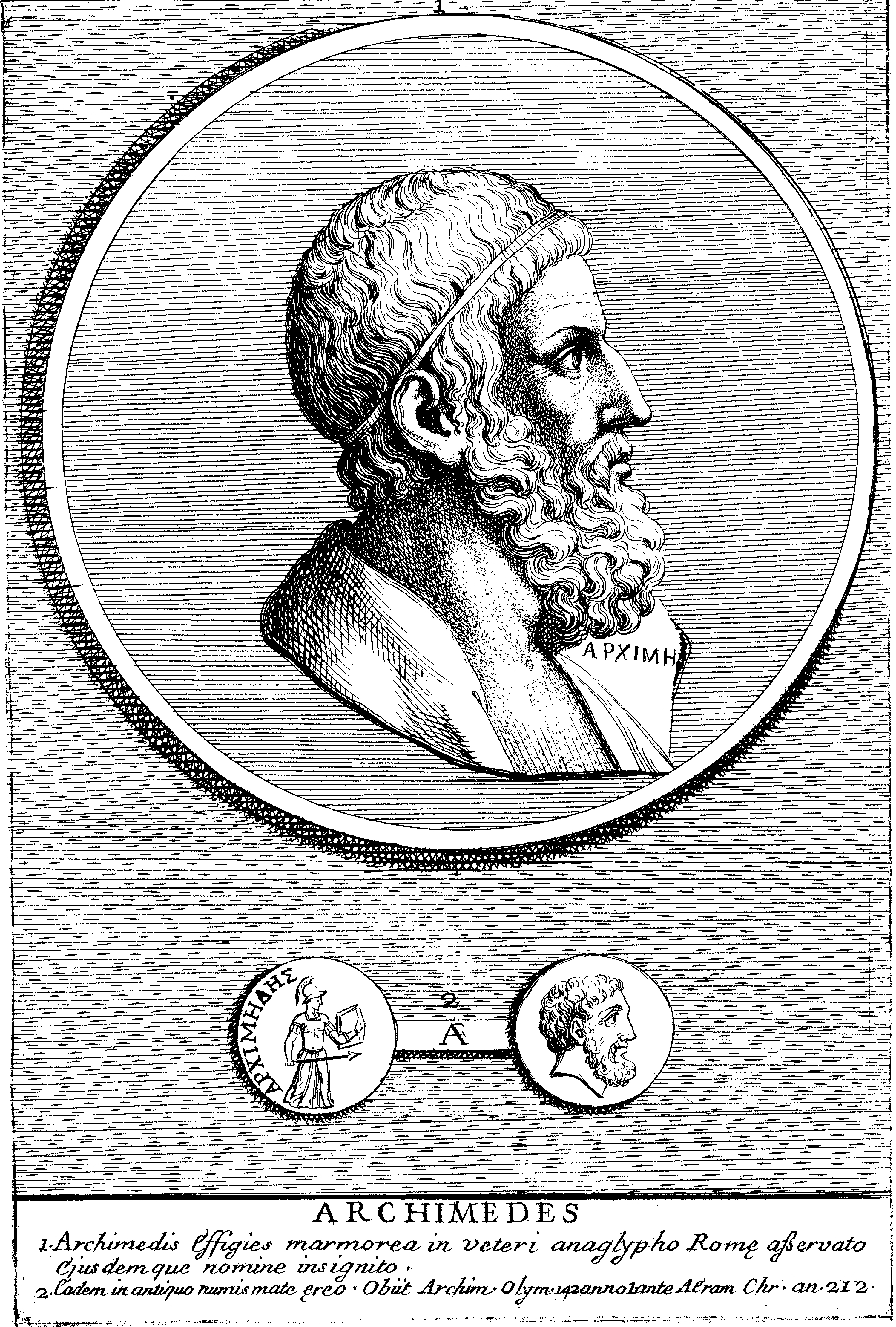
Every circle -- no matter if it fits in the palm of your hand or spans a
stadium -- has the same ratio of circumference to diameter. That ratio is
pi. Ancient peoples sensed something special here. The Babylonians (around
1900 BCE) used pi ~ 3.125. The Egyptians used a value close to 3.16. But
the first rigorous estimate came from Archimedes of Syracuse (around
250 BCE), who trapped the circle between inscribed and circumscribed
polygons with 96 sides and proved [@heath1897]:
$$3.1408 < \pi < 3.1429$$
```{python}
#| echo: false
from pathlib import Path; import urllib.request
_d = Path('images'); _d.mkdir(exist_ok=True)
_p = _d / 'james_gregory.jpg'
if not _p.exists():
try: urllib.request.urlretrieve('https://upload.wikimedia.org/wikipedia/commons/6/6c/James_Gregory_by_John_Scougal.jpg', _p)
except Exception: pass
```
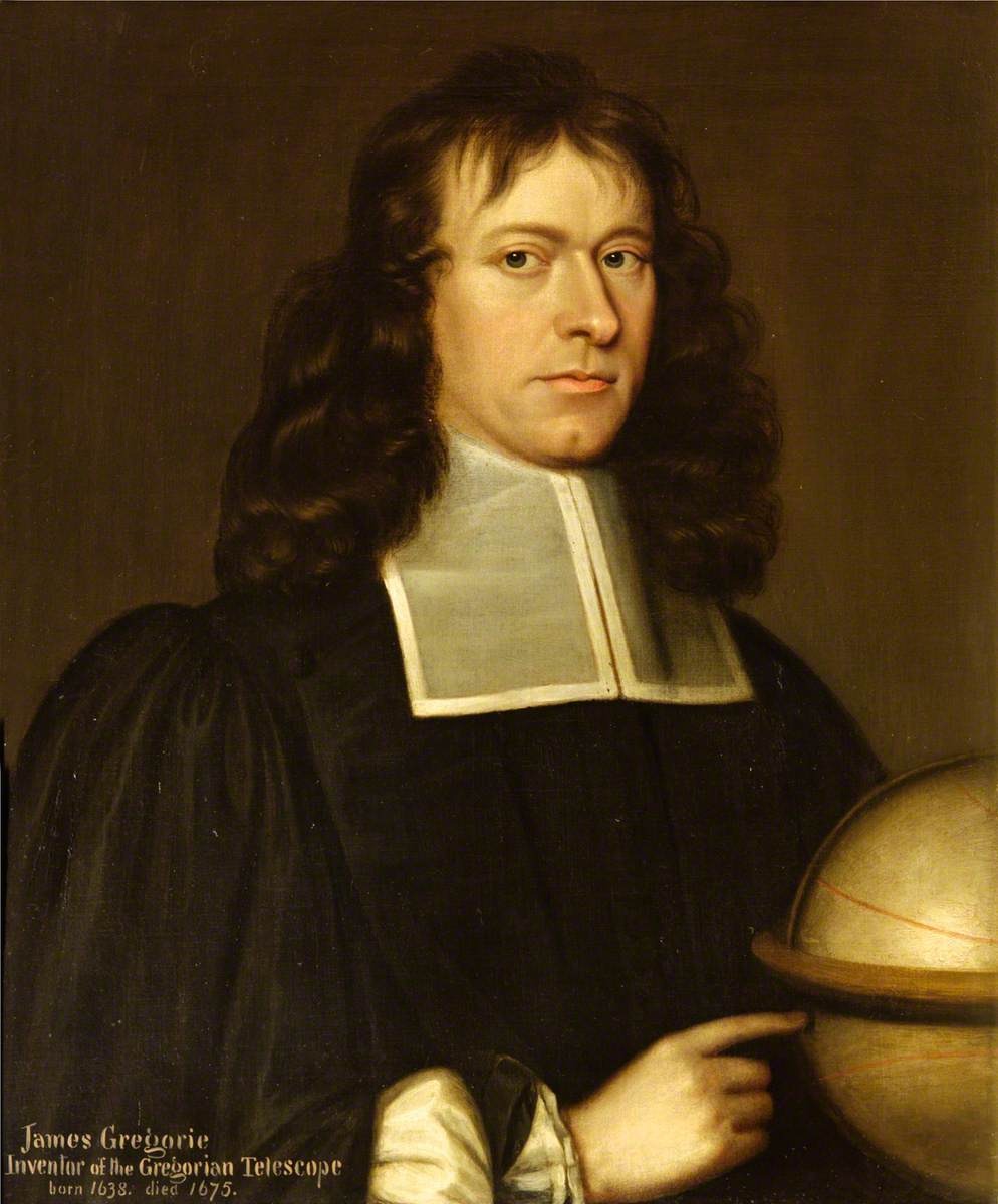
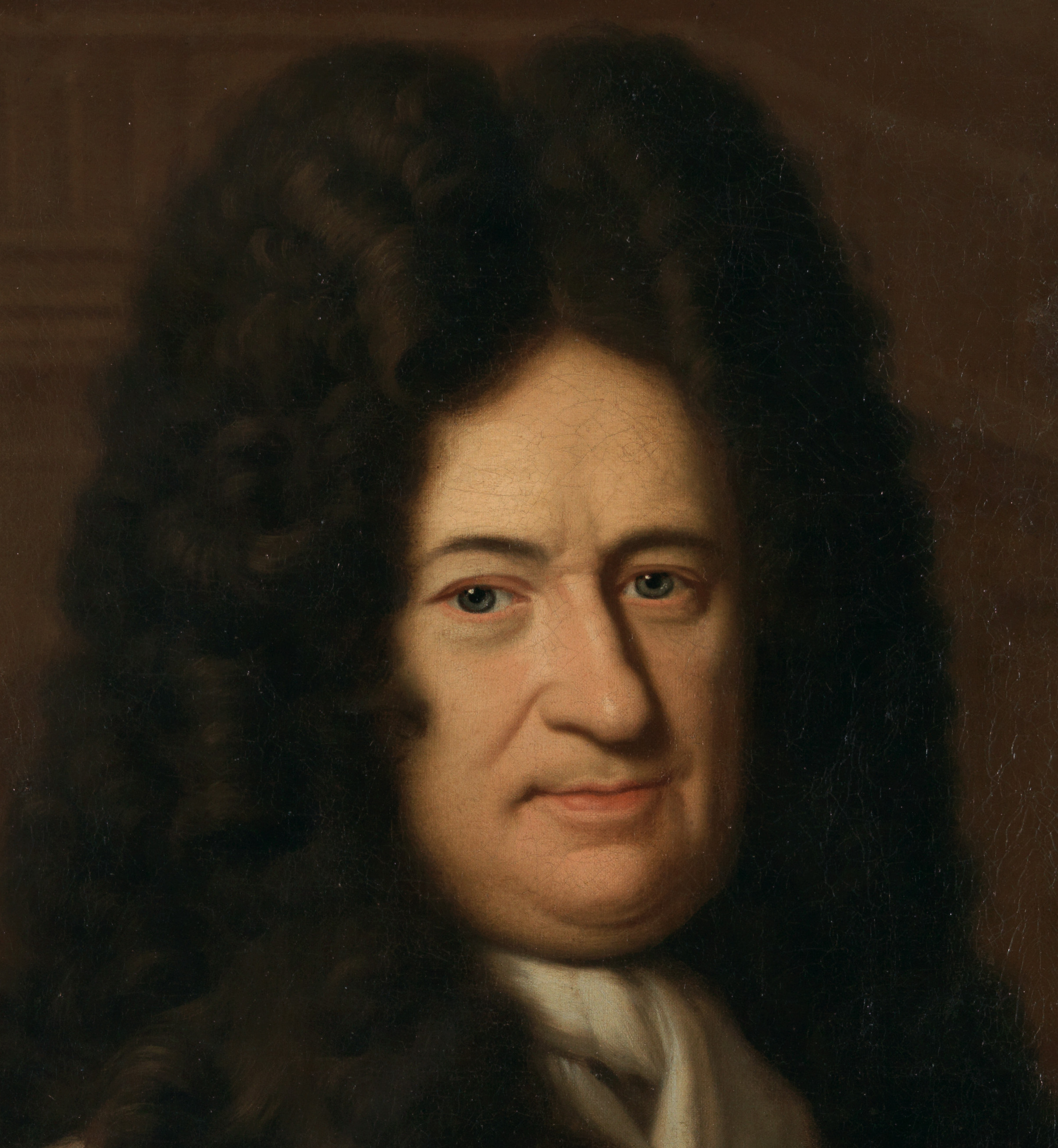
In 1671, James Gregory (and independently Leibniz in 1674) discovered a
beautiful but agonizingly slow series. Since arctan(1) = pi/4:
$$\frac{\pi}{4} = 1 - \frac{1}{3} + \frac{1}{5} - \frac{1}{7} + \cdots$$
The formula is exact -- add infinitely many terms and you get pi. The
catch: this series converges so slowly that you need millions of terms to
get just five correct decimal places.
```{python}
import math

def gregory_pi(n_terms):
    """pi/4 = 1 - 1/3 + 1/5 - ... (Gregory-Leibniz series)."""
    total = 0.0
    for k in range(n_terms):
        total += (-1)**k / (2*k + 1)
    return 4 * total
# uses: gregory_pi()
import math

true_pi = math.pi
print(f"{'Method':<18} {'approximation':>17}  error")
print("-" * 50)
for n in [100, 1000, 10000, 100000]:
    val = gregory_pi(n)
    err = abs(val - true_pi)
    print(f"Gregory({n:7d})  {val:.15f}  {err:.2e}")
print(f"{'True pi':<18} {true_pi:.15f}")
```
Accuracy creeps forward by one decimal place for every tenfold increase
in terms. At this rate, computing pi to 100 decimal places would require
more terms than atoms in the universe.
::: {.content-visible when-format="pdf"}
```{=latex}
\begin{center}
\begin{minipage}[c]{0.28\textwidth}\centering
\href{https://youtu.be/gMlf1ELvRzc}{\includegraphics[width=\textwidth]{images/thumb_gMlf1ELvRzc.jpg}}
\end{minipage}%
\hspace{0.02\textwidth}%
\begin{minipage}[c]{0.28\textwidth}
\small\textbf{Veritasium}\\[3pt]
\small The Discovery That Transformed Pi\\[3pt]
\small\href{https://youtu.be/gMlf1ELvRzc}{\texttt{youtu.be/gMlf1ELvRzc}}
\end{minipage}%
\hspace{0.02\textwidth}%
\begin{minipage}[c]{0.36\textwidth}
\small From Archimedes' polygons to Newton's infinite series — how a single insight turned pi from an unreachable mystery into a number you can compute to any precision you want.
\end{minipage}
\end{center}
```
:::
::: {.content-visible when-format="html"}
<div style="display:flex; align-items:flex-start; margin:1em 0; gap:12px; width:100%;">
<div style="flex:0 0 200px;"><a href="https://youtu.be/gMlf1ELvRzc" target="_blank"><img src="https://img.youtube.com/vi/gMlf1ELvRzc/0.jpg" style="width:100%;display:block;" alt="The Discovery That Transformed Pi"></a></div>
<div style="flex:1; font-size:0.85em;"><strong>Veritasium</strong><br>The Discovery That Transformed Pi<br><a href="https://youtu.be/gMlf1ELvRzc" target="_blank" style="font-family:monospace;">youtu.be/gMlf1ELvRzc</a></div>
<div style="flex:1; font-size:0.85em;">From Archimedes' polygons to Newton's infinite series — how a single insight turned pi from an unreachable mystery into a number you can compute to any precision you want.</div>
</div>
:::
```{python}
#| echo: false
from pathlib import Path; import urllib.request
_d = Path('images'); _d.mkdir(exist_ok=True)
_p = _d / 'lambert.png'
if not _p.exists():
try: urllib.request.urlretrieve('https://upload.wikimedia.org/wikipedia/commons/1/1d/Johann_Heinrich_Lambert_1829_Engelmann.png', _p)
except Exception: pass
```
```{python}
#| echo: false
from pathlib import Path; import urllib.request
_d = Path('images'); _d.mkdir(exist_ok=True)
_p = _d / 'lindemann.jpg'
if not _p.exists():
try: urllib.request.urlretrieve('https://upload.wikimedia.org/wikipedia/commons/b/bf/Carl_Louis_Ferdinand_von_Lindemann.jpg', _p)
except Exception: pass
```
::: {.content-visible when-format="pdf"}
```{=latex}
\begin{center}
\begin{minipage}[t]{0.38\textwidth}\centering
\includegraphics[width=0.85\textwidth]{images/lambert.png}\\[4pt]
\small\textit{Johann Heinrich Lambert (1728--1777)}\\[2pt]
\tiny Public domain, Godefroy Engelmann, via Wikimedia Commons
\end{minipage}%
\hspace{0.06\textwidth}%
\begin{minipage}[t]{0.38\textwidth}\centering
\includegraphics[width=0.85\textwidth]{images/lindemann.jpg}\\[4pt]
\small\textit{Ferdinand von Lindemann (1852--1939)}\\[2pt]
\tiny Public domain, via Wikimedia Commons
\end{minipage}
\end{center}
```
:::
::: {.content-visible when-format="html"}
<div style="display:flex; justify-content:center; gap:24px; margin:1em 0;">
<div style="text-align:center; max-width:160px;"><img src="images/lambert.png" style="width:140px;" alt="Johann Heinrich Lambert"><br><em style="font-size:0.82em;">Johann Heinrich Lambert (1728–1777)</em><br><span style="font-size:0.72em;">Public domain, Godefroy Engelmann, via Wikimedia Commons</span></div>
<div style="text-align:center; max-width:160px;"><img src="images/lindemann.jpg" style="width:140px;" alt="Ferdinand von Lindemann"><br><em style="font-size:0.82em;">Ferdinand von Lindemann (1852–1939)</em><br><span style="font-size:0.72em;">Public domain, via Wikimedia Commons</span></div>
</div>
:::
Pi was proved irrational by Johann Lambert in 1761 [@lambert1761].
In 1882, Ferdinand von Lindemann proved pi is *transcendental* -- it
cannot be the root of any polynomial with integer coefficients [@lindemann1882].
One consequence: the ancient problem of "squaring the circle" has no
solution.
Today pi has been computed to over 100 trillion decimal digits. One of
the greatest open questions in mathematics is whether pi is *normal*: does
every digit 0-9 appear equally often? Computationally the answer looks
like yes -- but it has never been proved. We will test this conjecture in
@sec-constants-normal.
## Computing π: Machin's Formula {#sec-constants-machin}
```{python}
#| echo: false
from pathlib import Path; import urllib.request
_d = Path('images'); _d.mkdir(exist_ok=True)
_p = _d / 'john_machin.jpg'
if not _p.exists():
try: urllib.request.urlretrieve('https://mathshistory.st-andrews.ac.uk/Biographies/Machin/Machin.jpeg', _p)
except Exception: pass
```
::: {.content-visible when-format="pdf"}
```{=latex}
\begin{center}
\begin{minipage}[c]{0.22\textwidth}
\includegraphics[width=\textwidth]{images/john_machin.jpg}
\end{minipage}%
\hspace{0.03\textwidth}%
\begin{minipage}[c]{0.55\textwidth}
\small\textit{John Machin (1680--1751)}\\[2pt]
\tiny MacTutor History of Mathematics, University of St Andrews.\newline
\url{https://mathshistory.st-andrews.ac.uk/Biographies/Machin/}
\end{minipage}
\end{center}
```
:::
::: {.content-visible when-format="html"}
<div style="display:flex; align-items:center; margin:1em 0; gap:12px;">
<img src="images/john_machin.jpg" style="width:100px; flex-shrink:0;" alt="John Machin">
<div style="font-size:0.82em;"><em>John Machin (1680–1751)</em><br><span style="font-size:0.85em;">MacTutor History of Mathematics, University of St Andrews. <a href="https://mathshistory.st-andrews.ac.uk/Biographies/Machin/">mathshistory.st-andrews.ac.uk</a></span></div>
</div>
:::
In 1706, the English mathematician John Machin discovered an identity that
made computing pi dramatically faster [@borwein1987piagm, Ch. 1]:
$$\frac{\pi}{4} = 4\arctan\!\left(\frac{1}{5}\right) -
\arctan\!\left(\frac{1}{239}\right)$$
Why does this help? The Taylor series for arctan(x) is:
$$\arctan(x) = x - \frac{x^3}{3} + \frac{x^5}{5} - \frac{x^7}{7}
+ \cdots \quad (|x| \le 1)$$
The Gregory-Leibniz formula uses x = 1, the slowest case -- terms
decrease only as 1/(2k+1). Machin's formula uses x = 1/5 and x = 1/239,
which are much smaller, so x^(2k+1) shrinks by a factor of 25 or more
per step.
```{python}
def arctan_series(x, n_terms):
    """arctan(x) = x - x^3/3 + x^5/5 - ... (Taylor series)."""
    total = 0.0
    x_sq = x * x
    x_pow = x
    for k in range(n_terms):
        total += ((-1)**k * x_pow) / (2*k + 1)
        x_pow *= x_sq
    return total

def machin_pi(n_terms):
    """pi = 16*arctan(1/5) - 4*arctan(1/239)  (Machin, 1706)."""
    return 4 * (4*arctan_series(1/5, n_terms)
                - arctan_series(1/239, n_terms))

# uses: gregory_pi(), machin_pi()

g100k = gregory_pi(100000)
m5    = machin_pi(5)
m10   = machin_pi(10)

print(f"{'Method':<22}  {'approximation':17}  error")
print("-" * 57)
for name, val in [("Gregory (100000)", g100k),
                  ("Machin  ( 5 terms)", m5),
                  ("Machin  (10 terms)", m10)]:
    err = abs(val - true_pi)
    print(f"{name:<22}  {val:.15f}  {err:.2e}")
print(f"{'True pi':<22}  {true_pi:.15f}")
```
Five terms of Machin outperform 100,000 terms of Gregory. Ten terms
exhausts all the precision Python's standard float can hold. Machin used
his formula to compute pi to 100 decimal places by hand in 1706 -- a
record that stood for decades.
The key to Machin's formula is that 1/5 and 1/239 are both small
fractions, so the series for each arctan converges quickly. Arctan
identities like this (called Machin-like formulas) are still used in
record pi computations today, combined with the high-precision arithmetic
introduced in @sec-constants-mpmath.
## The BBP Formula: Extracting Any Digit of π {#sec-constants-bbp}
```{python}
#| echo: false
from pathlib import Path; import urllib.request
_d = Path('images'); _d.mkdir(exist_ok=True)
_p = _d / 'jonathan_borwein.jpg'
if not _p.exists():
try: urllib.request.urlretrieve('https://mathshistory.st-andrews.ac.uk/Biographies/Borwein_Jonathan/borwein_jonathan_3.jpg', _p)
except Exception: pass
```
```{python}
#| echo: false
from pathlib import Path; import urllib.request
_d = Path('images'); _d.mkdir(exist_ok=True)
_p = _d / 'david_bailey.jpg'
if not _p.exists():
try:
_req = urllib.request.Request('https://upload.wikimedia.org/wikipedia/commons/2/23/David_Harold_Bailey.jpg', headers={'User-Agent': 'Mozilla/5.0 (educational-book-project)'})
with urllib.request.urlopen(_req) as _resp: _p.write_bytes(_resp.read())
except Exception: pass
```
```{python}
#| echo: false
from pathlib import Path; import urllib.request
_d = Path('images'); _d.mkdir(exist_ok=True)
_p = _d / 'simon_plouffe.jpg'
if not _p.exists():
try:
_req = urllib.request.Request('https://upload.wikimedia.org/wikipedia/commons/9/96/Simon_Plouffe_1.jpg', headers={'User-Agent': 'Mozilla/5.0 (educational-book-project)'})
with urllib.request.urlopen(_req) as _resp: _p.write_bytes(_resp.read())
except Exception: pass
```
::: {.content-visible when-format="pdf"}
```{=latex}
\begin{center}
\begin{minipage}[t]{0.28\textwidth}\centering
\includegraphics[width=0.85\textwidth]{images/jonathan_borwein.jpg}\\[4pt]
\small\textit{Jonathan Borwein (1951--2016)}\\[2pt]
\tiny Photo: \url{https://mathscholar.org/2017/03/jonathan-borwein-dies-at-65/}
\end{minipage}%
\hspace{0.04\textwidth}%
\begin{minipage}[t]{0.28\textwidth}\centering
\includegraphics[width=0.85\textwidth]{images/david_bailey.jpg}\\[4pt]
\small\textit{David H. Bailey (b.\ 1948)}\\[2pt]
\tiny CC BY-SA 3.0, Raul654, via Wikimedia Commons
\end{minipage}%
\hspace{0.04\textwidth}%
\begin{minipage}[t]{0.28\textwidth}\centering
\includegraphics[width=0.85\textwidth]{images/simon_plouffe.jpg}\\[4pt]
\small\textit{Simon Plouffe (b.\ 1956)}\\[2pt]
\tiny CC BY-SA 4.0, Plouffe (own work), via Wikimedia Commons
\end{minipage}
\end{center}
```
:::
::: {.content-visible when-format="html"}
<div style="display:flex; justify-content:center; gap:24px; margin:1em 0; flex-wrap:wrap;">
<div style="text-align:center; max-width:160px;">
<img src="images/jonathan_borwein.jpg" style="width:120px;" alt="Jonathan Borwein">
<div style="font-size:0.82em; margin-top:6px;"><em>Jonathan Borwein (1951–2016)</em><br><span style="font-size:0.85em;">Photo: <a href="https://mathscholar.org/2017/03/jonathan-borwein-dies-at-65/">mathscholar.org</a></span></div>
</div>
<div style="text-align:center; max-width:160px;">
<img src="images/david_bailey.jpg" style="width:120px;" alt="David H. Bailey">
<div style="font-size:0.82em; margin-top:6px;"><em>David H. Bailey (b. 1948)</em><br><span style="font-size:0.85em;">CC BY-SA 3.0, Raul654, via Wikimedia Commons</span></div>
</div>
<div style="text-align:center; max-width:160px;">
<img src="images/simon_plouffe.jpg" style="width:120px;" alt="Simon Plouffe">
<div style="font-size:0.82em; margin-top:6px;"><em>Simon Plouffe (b. 1956)</em><br><span style="font-size:0.85em;">CC BY-SA 4.0, Plouffe (own work), via Wikimedia Commons</span></div>
</div>
</div>
:::
In 1995, David Bailey, Peter Borwein, and Simon Plouffe made a discovery
that astonished mathematicians. Using an algorithm called PSLQ to search
for relationships among mathematical constants, they found [@bailey1997bbp; @borwein2009crucible, Ch. 2]:
$$\pi = \sum_{k=0}^{\infty} \frac{1}{16^k} \left( \frac{4}{8k+1}
- \frac{2}{8k+4} - \frac{1}{8k+5} - \frac{1}{8k+6} \right)$$
This is the **BBP formula**. The remarkable property: you can compute any
*hexadecimal* digit of pi directly, without computing any of the preceding
digits. Before 1995, no formula with this property was known for pi.
First, let us see how rapidly it converges:
```{python}
import math

def bbp_pi(n_terms):
    """Approximate pi via the BBP formula (1995)."""
    total = 0.0
    for k in range(n_terms):
        inv16k = 1.0 / (16**k)
        total += inv16k * (4/(8*k+1) - 2/(8*k+4)
                           - 1/(8*k+5) - 1/(8*k+6))
    return total

# uses: bbp_pi()

print(f"{'Terms':>6}  {'BBP approximation':>17}  error")
print("-" * 42)
for n in [3, 5, 8, 12]:
    val = bbp_pi(n)
    err = abs(val - true_pi)
    print(f"{n:6d}  {val:.15f}  {err:.2e}")
print(f"{'True':>6}  {true_pi:.15f}")
```
Each additional term reduces the error by a factor of about 16 --
far faster than Machin's formula and astronomically faster than Gregory's.
Now for the digit-extraction algorithm. If we multiply the BBP sum by
16^d and keep only the fractional part, we get the hexadecimal digits of
pi starting at position d+1. The key trick is that `pow(16, n, m)` from
@sec-modular-operator computes 16^n mod m instantly, no matter how large
n is, so we never store the enormous number 16^n.
```{python}
import math

def _bbp_s(j, d):
    """Fractional part of 16^d * sum_{k>=0} 1/(16^k * (8k+j))."""
    s = 0.0
    # Finite sum: apply pow(b,n,m) from @sec-modular-operator
    for k in range(d + 1):
        denom = 8*k + j
        s += pow(16, d - k, denom) / denom
        s -= math.floor(s)
    # Rapidly convergent tail
    power = 1.0 / 16.0
    for k in range(d + 1, d + 100):
        t = power / (8*k + j)
        if t < 1e-17:
            break
        s += t
        s -= math.floor(s)
        power /= 16.0
    return s

def bbp_hex(d, length=8):
    """Return 'length' hex digits of pi starting at position d+1.
    d=0 gives the first 'length' digits after the decimal point.
    """
    x = (4*_bbp_s(1, d) - 2*_bbp_s(4, d)
         - _bbp_s(5, d) - _bbp_s(6, d))
    x -= math.floor(x)
    hx = "0123456789ABCDEF"
    result = ""
    for _ in range(length):
        x *= 16
        digit = int(x)
        result += hx[digit]
        x -= digit
    return result

# uses: bbp_hex()
import math

# pi in hex: 3.243F6A8885A308D3...
print("First 14 hex digits of pi:")
print("  Computed:", bbp_hex(0, 14))
print("  Expected: 243F6A8885A308")

print()
# Compute hex digits at position 1,000,000
# (skipping past the first 999,999 digits entirely)
print("Hex digits at position 1,000,000:")
print("  Computed:", bbp_hex(999999, 14))
# Borwein et al. (EMA 2006) Table 2.1:
print("  Expected: 26C65E52CB4593")
```
In roughly a second, Python computes hexadecimal digits of pi at position
one million -- without ever computing the preceding 999,999 digits. This
was the first time in history that pi's digits could be extracted
surgically at any desired location.
The PSLQ algorithm that *discovered* the BBP formula is itself remarkable.
It takes a list of real numbers and finds integer relationships among them.
Bailey, Borwein, and Plouffe fed PSLQ a list of constants of a specific
algebraic form, and it returned the BBP formula as the unique combination
equal to pi [@bailey1997bbp].
## The Algorithm Race {#sec-constants-race}
All three formulas converge to pi, but at wildly different speeds.
### Research Example: Racing to $\pi$ — Which Formula Wins? {.unnumbered .unlisted}
**Proposal.** Gregory, Machin, and BBP all compute the same number, but at
shockingly different speeds. Can we put all three on one graph and *see*
exactly how fast each closes in on the true value?
```{python}
#| label: fig-pi-race
#| fig-cap: "Gregory crawls (polynomial convergence); Machin and BBP plummet (exponential). Ten terms of either beats 100,000 terms of Gregory."
# uses: gregory_pi(), machin_pi(), bbp_pi()
import matplotlib.pyplot as plt
import math

BLUE = '#1f77b4'
RED  = '#d62728'

true_pi = math.pi

greg_n = [10, 50, 100, 500, 1000, 5000, 10000, 50000, 100000]
greg_e = [abs(gregory_pi(n) - true_pi) for n in greg_n]

mach_n = list(range(1, 13))
mach_e = [abs(machin_pi(n) - true_pi) for n in mach_n]

bbp_n  = list(range(1, 13))
bbp_e  = [max(abs(bbp_pi(n) - true_pi), 1e-16) for n in bbp_n]

fig, (ax1, ax2) = plt.subplots(1, 2, figsize=(10, 4))

ax1.loglog(greg_n, greg_e, 'o-', color=BLUE)
ax1.set_title("Gregory-Leibniz")
ax1.set_xlabel("Terms used")
ax1.set_ylabel("|error|")
ax1.text(50, 0.003,
         "slope = −1\n(one digit per\n10× more terms)",
         fontsize=8)

ax2.semilogy(mach_n, mach_e, 's--',
             label='Machin (×25/term)', color=BLUE)
ax2.semilogy(bbp_n, bbp_e, '^:',
             label='BBP (×16/term)', color=RED)
ax2.set_title("Machin vs BBP")
ax2.set_xlabel("Terms used")
ax2.legend()

fig.suptitle("Racing to π: how fast does each formula converge?")
plt.tight_layout()
plt.show()
```
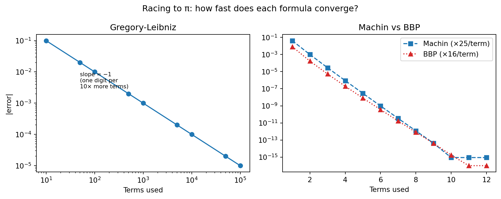
Gregory's error shrinks by a factor of 10 for every tenfold increase in
terms -- that is the straight slope-−1 line on the left log-log plot.
Machin's error shrinks by a factor of 25 per term; BBP's by a factor of
16. Both plummet so fast that the right panel looks almost vertical. Ten
terms of Machin exhausts 64-bit floating-point precision. The same is true
of BBP. For Gregory to reach that precision would require roughly $10^{14}$
terms -- a computation that would take longer than the age of the universe
on a modern CPU.
This convergence race is why algorithm choice is not a minor detail in
computational mathematics. Two formulas for the same answer can differ by
a factor of a trillion in efficiency. You just saw that gap with your own
eyes in 30 lines of Python.
## Testing Normality of $\pi$'s Digits {#sec-constants-normal}
A number is **normal** (in base 10) if every digit 0-9 appears with equal
long-run frequency, every two-digit block appears equally often, and so on
for every block length [@martin2011, §2.3].
Two numbers are known to be normal:
- **Champernowne's constant** (0.1234567891011121314...): constructed by
concatenating all positive integers [@champernowne1933].
- The **Copeland-Erdős constant** (0.235711131719...): constructed by
concatenating all primes [@copeland1946].
Pi is strongly *conjectured* to be normal, but no proof exists. Let us
test the conjecture on the first 1,000 decimal digits.
To get 1,000 digits of pi, we use the `mpmath` library. It provides
arbitrary-precision arithmetic -- you can set the number of decimal places
to any value you want. We introduce it briefly here; @sec-constants-mpmath
gives a fuller treatment.
```{python}
import mpmath

# mp.dps is the number of decimal places of precision
mpmath.mp.dps = 1010  # 1000 digits plus a safety buffer

# mpmath.pi is pi at the current precision
pi_str = mpmath.nstr(mpmath.pi, 1002)

# The string looks like "3.14159265..."; drop "3." to get digits
after_dec = pi_str.split(".")[1][:1000]

print(f"Digits collected: {len(after_dec)}")
print("First 50 digits of pi:")
print(" ", after_dec[:50])
print()
print(f"{'Digit':>5}  {'Count':>5}  {'%':>6}  (expected 10.0%)")
print("-" * 40)
for d in "0123456789":
    n = after_dec.count(d)
    pct = n / 10.0
    print(f"  {d}:     {n:4d}   {pct:5.1f}%")
```
No digit is dramatically over- or under-represented. The frequencies hover
near 10% exactly as normality predicts, though none is exactly 100 out of
1,000 (just as flipping a fair coin 1,000 times rarely gives exactly 500
heads).
### Research Example: Are $\pi$'s First 1000 Digits Normal? {.unnumbered .unlisted}
**Proposal.** Normality predicts every digit 0–9 should appear equally
often. Can a bar chart and a chi-squared score tell us whether pi's
first 1,000 decimal digits pass that test?
```{python}
#| label: fig-pi-normality
#| fig-cap: "Digit frequencies in the first 1,000 decimal digits of pi. Each bar is within a few counts of the expected 100 -- tantalizing evidence for normality."
import matplotlib.pyplot as plt
import mpmath

BLUE = '#1f77b4'
RED  = '#d62728'

mpmath.mp.dps = 1010
pi_str = mpmath.nstr(mpmath.pi, 1002)
after_dec = pi_str.split(".")[1][:1000]

digits = list("0123456789")
observed = [after_dec.count(d) for d in digits]
expected = [100] * 10

chi2 = sum((o - e)**2 / e for o, e in zip(observed, expected))

fig, ax = plt.subplots(figsize=(7, 4))
x = range(10)
ax.bar([i - 0.2 for i in x], observed, width=0.4,
       label="Observed", color=BLUE)
ax.bar([i + 0.2 for i in x], expected, width=0.4,
       label="Expected (normal)", color=RED, alpha=0.7)
ax.set_xticks(list(x))
ax.set_xticklabels(digits)
ax.set_xlabel("Digit")
ax.set_ylabel("Count (per 1000 digits of pi)")
ax.set_title(
    f"Digit frequency in the first 1000 decimal digits of pi"
    f"  (χ² = {chi2:.1f}, 9 df)"
)
ax.legend()
plt.tight_layout()
plt.show()
print(f"Chi-squared statistic: {chi2:.2f}  (9 degrees of freedom)")
print("p-value threshold for 95% confidence: 16.92")
print(f"Pi's digit distribution {'passes' if chi2 < 16.92 else 'fails'}"
      " the chi-squared test at 95% confidence.")
```
The bars cluster tightly around 100 — no digit is dramatically over- or
under-represented. The chi-squared value comfortably clears the 95%
threshold, which is exactly what we would expect from a normal number.
Whether pi is truly normal remains one of the most celebrated open
problems in number theory — and you just ran the statistical test yourself
in fewer than 20 lines of Python.
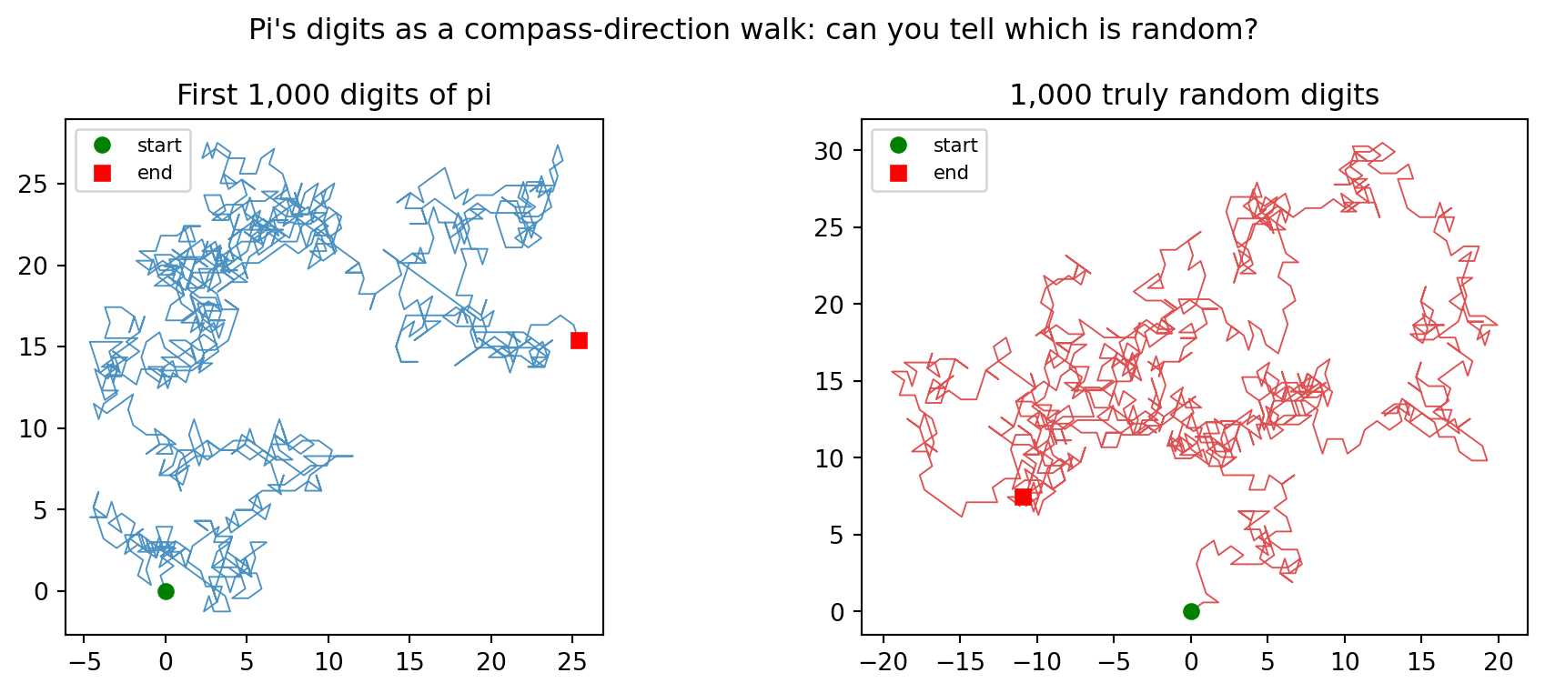
### Research Example: $\pi$'s Digits as a Random Walk {.unnumbered .unlisted}
**Proposal.** If pi's digits are truly random, treating each digit as a
compass direction should produce a walk that looks just like a walk driven
by a random-number generator. Can we see this with our own eyes?
```{python}
#| label: fig-pi-walk
#| fig-cap: "Pi's digits as compass directions (left) versus a walk driven by a true random-number generator (right). The two paths look statistically indistinguishable — exactly what normality predicts."
import matplotlib.pyplot as plt
import mpmath
import random
import math

BLUE  = '#1f77b4'
RED   = '#d62728'

mpmath.mp.dps = 1010
pi_str    = mpmath.nstr(mpmath.pi, 1002)
pi_digits = [int(d) for d in pi_str.replace('.', '')[:1000]]

def digit_walk(digits):
    x, y = [0.0], [0.0]
    for d in digits:
        angle = d * 36 * math.pi / 180
        x.append(x[-1] + math.cos(angle))
        y.append(y[-1] + math.sin(angle))
    return x, y

random.seed(42)
rand_digits = [random.randint(0, 9) for _ in range(1000)]

fig, (ax1, ax2) = plt.subplots(1, 2, figsize=(10, 4))

xp, yp = digit_walk(pi_digits)
ax1.plot(xp, yp, color=BLUE, lw=0.7, alpha=0.8)
ax1.plot(xp[0], yp[0], 'go', ms=6, label='start')
ax1.plot(xp[-1], yp[-1], 'rs', ms=6, label='end')
ax1.set_title("First 1,000 digits of pi")
ax1.set_aspect('equal')
ax1.legend(fontsize=8)

xr, yr = digit_walk(rand_digits)
ax2.plot(xr, yr, color=RED, lw=0.7, alpha=0.8)
ax2.plot(xr[0], yr[0], 'go', ms=6, label='start')
ax2.plot(xr[-1], yr[-1], 'rs', ms=6, label='end')
ax2.set_title("1,000 truly random digits")
ax2.set_aspect('equal')
ax2.legend(fontsize=8)

fig.suptitle("Pi's digits as a compass-direction walk: can you tell which is random?")
plt.tight_layout()
plt.show()
```
The two paths twist through space in ways that look statistically identical
— your eye cannot tell which is driven by pi's digits and which by a
random-number generator. That is exactly what normality predicts. Try
repeating the walk with the digits of *e* or *sqrt(2)*: do those constants
look equally "random"?
## Other Constants: $e$, $\sqrt{2}$, the Golden Ratio {#sec-constants-others}
Pi has famous companions. Each constant tells a different story, and their
continued-fraction (CF) expansions reveal striking patterns. The CF
algorithm below is adapted from @sec-cfrac-algorithm:
```{python}
def to_cf(x, n_terms):
    """Continued fraction expansion of x (float version)."""
    result = []
    for _ in range(n_terms):
        a = int(x)
        result.append(a)
        frac = x - a
        if frac < 1e-10:
            break
        x = 1.0 / frac
    return result

# Golden ratio phi (see @sec-fib-golden)
phi = (1 + math.sqrt(5)) / 2

constants = [
    ("pi",      math.pi),
    ("e",       math.e),
    ("sqrt(2)", math.sqrt(2)),
    ("phi",     phi),
    ("ln(2)",   math.log(2)),
]

print(f"{'Constant':<10}  CF expansion (first 12 terms)")
print("-" * 55)
for name, val in constants:
    cf = to_cf(val, 12)
    print(f"{name:<10}  {cf}")
```
The patterns stand out:
- **Phi** [1;1,1,1,...]: all partial quotients equal 1, making phi the
"hardest to approximate" by rationals (see @sec-cfrac-golden). This is
why flower petals grow in Fibonacci numbers.
- **e** [2;1,2,1,1,4,1,1,6,...]: a provably beautiful pattern
[2;1,2k,1,1,4k,...]. Among well-known constants, e is one of the rare
ones whose CF expansion is fully understood.
- **sqrt(2)** [1;2,2,2,...]: purely periodic, exactly as Lagrange's
theorem predicts for quadratic irrationals (see @sec-cfrac-periodic).
The convergents p/q give the best solutions to Pell's equation x^2 - 2y^2 = 1.
- **Pi** [3;7,15,1,292,...]: no known pattern. The unusually large term
292 means that 355/113 = 3.14159292... is an exceptional rational
approximation -- accurate to 7 decimal places with a denominator of
only 113.
How do mathematicians identify a mysterious decimal? Tools like the
Inverse Symbolic Calculator (ISC) and the `mpmath.identify` function
maintain databases of known constants and their decimal expansions. Given
a sufficiently precise decimal, they can guess a closed form. This is
exactly the technology that guided the search leading to the BBP formula:
PSLQ scanned linear combinations of known constants until pi emerged [@borwein2009crucible, Ch. 3].
## High-Precision Arithmetic with mpmath {#sec-constants-mpmath}
Python's standard `float` stores a number in 64 bits, giving about 15-16
significant decimal digits. That is more than enough for engineering, but
experimental mathematicians often need hundreds or thousands of digits to
distinguish a pattern from a coincidence, or to discover a new identity.
The `mpmath` library provides **arbitrary-precision arithmetic**. You
choose the number of decimal places (`mp.dps`) and mpmath keeps all
computations accurate to that many digits. Internally it uses algorithms
that scale efficiently to millions of digits.
```{python}
import mpmath

# mp.dps controls decimal-place precision globally
for dps in [15, 30, 50]:
    mpmath.mp.dps = dps
    label = f"mp.dps = {dps}"
    # width=60 wraps long output to fit the printed page
    import textwrap
    val = mpmath.nstr(mpmath.pi, dps)
    print(f"{label}:")
    print(textwrap.fill(val, width=60))
    print()
```
Beyond pi, mpmath knows a wide range of mathematical constants:
```{python}
mpmath.mp.dps = 35

constants_mp = [
    ("pi",              mpmath.pi),
    ("e",               mpmath.e),
    ("phi",             mpmath.phi),
    ("sqrt(2)",         mpmath.sqrt(2)),
    ("ln(2)",           mpmath.log(2)),
    ("Euler-Mascheroni", mpmath.euler),
    ("Catalan",         mpmath.catalan),
]

print(f"{'Constant':<22}  Value (35 decimal places)")
print("-" * 68)
for name, val in constants_mp:
    print(f"{name:<22}  {mpmath.nstr(val, 30)}")
```
Now let us revisit Machin's formula with mpmath arithmetic. With standard
floats, Machin(10) exhausts 64-bit precision. With mpmath, we can push as
far as we like:
```{python}
mpmath.mp.dps = 55  # 5-digit safety buffer for 50-digit result

def machin_mpmath(n_terms):
    """Machin's formula using mpmath for arbitrary precision."""
    a5 = mpmath.mpf(0)
    a239 = mpmath.mpf(0)
    x5   = mpmath.mpf(1) / 5
    x239 = mpmath.mpf(1) / 239
    p5   = x5
    p239 = x239
    for k in range(n_terms):
        sign = (-1)**k
        a5   += sign * p5   / (2*k + 1)
        a239 += sign * p239 / (2*k + 1)
        p5   *= x5 * x5
        p239 *= x239 * x239
    return 4 * (4*a5 - a239)

result = machin_mpmath(40)
err = abs(result - mpmath.pi)

print("Machin (40 terms) at 50+ digits:")
# width=60 wraps long output to fit the printed page
import textwrap
print(textwrap.fill(mpmath.nstr(result, 52), width=60))
print()
print("Error vs mpmath.pi:")
print(mpmath.nstr(err, 3))
```
Forty terms of the Machin series, computed in mpmath, agree with
`mpmath.pi` to all 50 requested digits. This is experimental mathematics
at work: we verify a known formula at increasing precision and confirm
that it keeps matching.
A practical rule of thumb: every 15 additional terms of Machin's
arctan(1/5) series buys roughly 10 extra digits of pi. Choosing the number
of terms to match your target precision is itself an interesting
optimization problem (see the research topics below).
## Further Research Topics {#sec-constants-research}
The following problems are listed roughly in order of increasing
difficulty. The first few are suitable for a class session; the last
several are open-ended research directions.
1. **Visualizing Gregory's error.** Plot the error `|gregory_pi(n) - pi|`
on a log-log plot for n = 10, 100, 1000, ..., 10^7. What is the slope?
How does this confirm the O(1/n) convergence rate? Repeat for Machin's
formula.
*(Problem proposed by Claude Code.)*
2. **Niven's constant curiosity.** Compute `sum(1/k**2 for k in range(1,
n+1))` for large n and compare to mpmath's value of `pi**2/6`. How
many digits match after 10^4 terms? 10^6 terms? Relate this to the
convergence rate of the Basel series.
*(Problem proposed by Claude Code.)*
3. **Verify Euler's identity [@hardywright1979].** Use mpmath to compute `mpmath.exp(1j *
mpmath.pi) + 1` (where `1j` is Python's imaginary unit). Do the real
and imaginary parts equal 0 to your precision? Increase `mp.dps` and
check when numerical noise becomes visible.
*(Problem proposed by Claude Code.)*
4. **Wallis product for pi.** In 1655, John Wallis [@wallis1656] discovered that
pi/2 = (2/1) * (2/3) * (4/3) * (4/5) * (6/5) * (6/7) * ....
Implement this as a running product and record the error after 10^2,
10^4, and 10^6 factor-pairs. Plot the error on a log-log scale and
find the slope. How does the convergence rate compare to Gregory's
series? Explain in terms of how fast the individual factors approach 1.
*(Problem proposed by Claude Code.)*
5. **Champernowne normality test.** Implement the Champernowne constant
[@champernowne1933] (concatenate integers 1, 2, 3, ...) using Python string operations.
Count digit frequencies in the first 10,000 digits. Does it look more
uniform than pi's first 10,000 digits? Why might that be?
*(Problem proposed by Claude Code.)*
6. **Copeland-Erdos constant.** Build the Copeland-Erdos constant [@copeland1946] by
concatenating primes (use `sympy.isprime` from @sec-primes-what). Test
normality on the first 2,000 digits. Compare the chi-squared statistic
against pi's first 2,000 digits.
*(Problem proposed by Claude Code.)*
7. **Machin-like formulas.** The formula pi/4 = arctan(1/2) + arctan(1/3)
is another Machin-like identity [@borwein1987piagm]. Implement it and measure how many
terms are needed for 15-digit accuracy. Compare to Machin's original
formula. Why does the choice of arctan arguments matter?
*(Problem proposed by Claude Code.)*
8. **BBP for other constants.** The number ln(2) has its own BBP-like
formula [@bailey1997bbp]: ln(2) = sum_{k=1}^{inf} 1/(k * 2^k). Implement hex digit
extraction for ln(2) and verify a few digits against `mpmath.log(2)`.
Can you find a BBP formula for ln(3)?
*(Problem proposed by Claude Code.)*
9. **Normality of other constants.** Using mpmath, extract 5,000 decimal
digits of e, sqrt(2), ln(2), and the golden ratio phi. Compute
chi-squared statistics for digit uniformity. Which constant looks most
normal? Least normal? Does this surprise you?
*(Problem proposed by Claude Code.)*
10. **The Gauss-Kuzmin distribution for pi.** Compute the continued
fraction of pi to 500 terms using `to_cf(math.pi, 500)`. Plot a
histogram of the partial quotient values. Compare to the Gauss-Kuzmin
distribution [@khinchin1964] from @sec-cfrac-gauss-kuzmin. Is pi's CF expansion
consistent with the distribution that "almost all" reals obey?
*(Problem proposed by Claude Code.)*
11. **BBP hex frequency test.** Use `bbp_hex` [@bailey1997bbp] to generate 500 consecutive
hex digits of pi (call it 500 times with d = 0, 8, 16, ...). Count
the frequencies of hex digits 0-F. Does pi's hex expansion look
"normal" in base 16? How many samples would you need to draw a
statistically meaningful conclusion?
*(Problem proposed by Claude Code.)*
12. **Rational approximations of pi.** The continued fraction
[3;7,15,1,292,...] produces the sequence of best rational
approximations: 3/1, 22/7, 333/106, 355/113, .... For each
convergent p/q, compute |pi - p/q| and compare to 1/(2q^2). Which
convergent first gives pi accurate to 10 significant figures? Research
why 355/113 was so important to Chinese and European astronomers before
calculus was invented.
*(Problem proposed by Claude Code.)*
13. **e digit patterns.** It is known [@hardywright1979] that e's continued fraction follows
the pattern [2;1,2,1,1,4,1,1,6,1,1,8,...]. Verify the pattern for
the first 50 terms using mpmath at 200 decimal places. At what term
does float64 precision cause the CF expansion to diverge from the
true pattern? Use this to illustrate why high precision matters.
*(Problem proposed by Claude Code.)*
14. **PSLQ in miniature.** Given a mystery decimal like
`mpmath.sqrt(2) + mpmath.pi / 4`, see if you can guess its closed
form by testing linear combinations a*pi + b*sqrt(2) + c*e with small
integer coefficients a, b, c [@borwein2009crucible]. How many decimal places do you need
before a random coincidence becomes a reliable identification?
*(Problem proposed by Claude Code.)*
15. **Spigot algorithms.** The Rabinowitz-Wagon "spigot" algorithm
[@rabinowitz1995] outputs digits of pi one at a time using only integer arithmetic.
Implement it and compare its output speed (digits per second) to
Machin's formula at the same precision. For what precision does
Machin outperform spigot?
*(Problem proposed by Claude Code.)*
16. **Ramanujan's series for 1/pi.** In 1914, Srinivasa Ramanujan [@ramanujan1914] wrote
down -- without proof -- the identity:
$$\frac{1}{\pi} = \frac{2\sqrt{2}}{9801}
\sum_{k=0}^{\infty}
\frac{(4k)!\,(1103 + 26390k)}{(k!)^4\,396^{4k}}$$
Each term contributes roughly 8 correct decimal digits of 1/pi.
Set `mp.dps = 100` and implement the series; verify against
`1 / mpmath.pi`. How many terms were needed? The Chudnovsky
brothers' algorithm (used by y-cruncher for world-record pi
computations) is a close relative of this formula. Research how
the two series differ and why the Chudnovsky variant converges
even faster.
*(Problem proposed by Claude Code.)*
17. **Feigenbaum's constant.** The logistic-map constant delta ~ 4.6692
[@feigenbaum1978] (see @sec-logistic) is conjectured but not proved to be transcendental.
Extract 200 decimal places using mpmath (it is built in as
`mpmath.feigenbaum`). Test its digit distribution. How does this
compare to pi? Does the apparent randomness tell you anything about
transcendence?
*(Problem proposed by Claude Code.)*
18. **Record pi computations.** Research the history of pi computation
milestones: from Machin (100 digits, 1706) to Shanks and Wrench
(100,000 digits, 1961) to the current trillion-plus digit records.
What algorithms (AGM, y-cruncher) enabled each leap? Write a brief
timeline and explain -- at a high level -- why fast multiplication
algorithms (FFT-based) are essential for extremely high precision
[@borwein1987piagm].
*(Problem proposed by Claude Code.)*
19. **The Euler-Mascheroni constant [@hardywright1979].** The limit
gamma = lim_{n->inf} (1 + 1/2 + 1/3 + ... + 1/n - ln n) ≈ 0.5772
is one of mathematics' most mysterious numbers; access it via
`mpmath.euler`. (a) Compute partial sums of the harmonic series minus
`mpmath.log(n)` for n = 10, 100, ..., 10^6 and plot convergence --
how many extra powers of 10 are needed to gain one more correct
digit? (b) Extract 5,000 digits of gamma and run the chi-squared
normality test from @sec-constants-normal. (c) Unlike pi and e, it
is not even proved that gamma is irrational. Research what that open
question means for normality conjectures, and find a recent expository
paper or blog post that describes the state of knowledge about gamma's
arithmetic nature.
*(Problem proposed by Claude Code.)*