# Continued Fractions: Fractions of Fractions {#sec-cfrac}
Decimals describe a number by recording how far each digit departs from
a power of ten. That works fine for everyday measurement, but it can
hide arithmetic structure. The decimal 3.14159... tells you almost
nothing about why 22/7 is such a good stand-in for pi, and 1.41421...
gives no hint that $\sqrt{2}$ has the most regular pattern of all
non-rational numbers. A completely different way of writing any
number -- the continued fraction -- lays that hidden structure bare.
The computer scientist Bill Gosper once described the experience of
reading a number through its continued fraction: "It's completely
astounding ... it looks like you are cheating God somehow." [@borwein2006ema, Ch. IX]
Every real number has a unique continued fraction, and the pattern of
its coefficients encodes how well the number can be approximated by
fractions -- one of the deepest questions in number theory.
## Beyond Decimal Expansions {#sec-cfrac-intro}
::: {.content-visible when-format="pdf"}
```{=latex}
\begin{center}
\begin{minipage}[c]{0.28\textwidth}\centering
\href{https://youtu.be/YCJ99liapCQ}{\includegraphics[width=\textwidth]{images/thumb_YCJ99liapCQ.jpg}}
\end{minipage}%
\hspace{0.02\textwidth}%
\begin{minipage}[c]{0.28\textwidth}
\small\textbf{Combo Class}\\[3pt]
\small Capturing Infinity With Fractions\\[3pt]
\small\href{https://youtu.be/YCJ99liapCQ}{\texttt{youtu.be/YCJ99liapCQ}}
\end{minipage}%
\hspace{0.02\textwidth}%
\begin{minipage}[c]{0.36\textwidth}
\small An enthusiastic tour of how infinite continued fractions trap irrational numbers exactly — using nothing but whole numbers and repeated division.
\end{minipage}
\end{center}
```
:::
::: {.content-visible when-format="html"}
<div style="display:flex; align-items:flex-start; margin:1em 0; gap:12px; width:100%;">
<div style="flex:0 0 200px;"><a href="https://youtu.be/YCJ99liapCQ" target="_blank"><img src="https://img.youtube.com/vi/YCJ99liapCQ/0.jpg" style="width:100%;" alt="Capturing Infinity With Fractions"></a></div>
<div style="flex:1; font-size:0.85em;"><strong>Combo Class</strong><br>Capturing Infinity With Fractions<br><a href="https://youtu.be/YCJ99liapCQ" target="_blank" style="font-family:monospace;">youtu.be/YCJ99liapCQ</a></div>
<div style="flex:1; font-size:0.85em;">An enthusiastic tour of how infinite continued fractions trap irrational numbers exactly — using nothing but whole numbers and repeated division.</div>
</div>
:::
A **simple continued fraction** is an expression of the form
$$x = a_0 + \cfrac{1}{a_1 + \cfrac{1}{a_2 + \cfrac{1}{a_3 + \cdots}}}$$
where $a_0$ is an integer (the integer part of $x$) and each
$a_1, a_2, a_3, \ldots$ is a **positive** integer. These numbers are
called the **partial quotients**. The compact notation is
$[a_0;\, a_1, a_2, a_3, \ldots]$.
Four examples span the range from simple to surprising:
| Number | Decimal | Continued fraction |
|--------|---------|-------------------|
| 22/7 | 3.142857... | [3; 7] |
| 355/113 | 3.141592... | [3; 7, 16] |
| $\sqrt{2}$ | 1.414213... | [1; 2, 2, 2, ...] |
| $\pi$ | 3.141592... | [3; 7, 15, 1, 292, ...] |
### Research Example: Why Does 355/113 Approximate $\pi$ So Freakishly Well? {.unnumbered .unlisted}
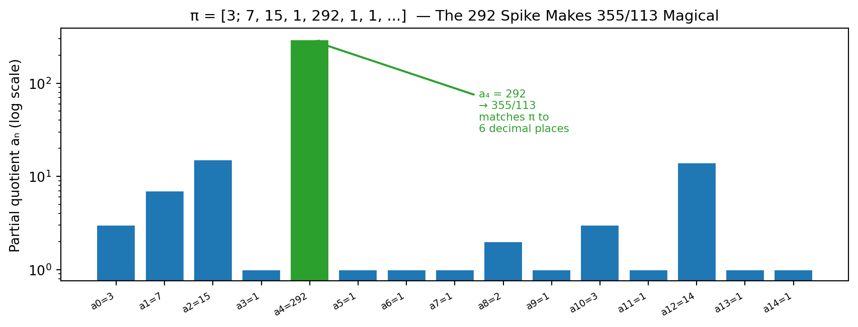
The table above lists 355/113 as matching π to six decimal places — yet its denominator is only 113. How can such a small fraction get so close? The continued fraction of π hides the answer in a single towering number: the partial quotient 292.
```{python}
#| label: fig-cfrac-spike
#| fig-cap: "Partial quotients of π on a log scale. The towering spike at position 4 — value 292 — is why 355/113 is so freakishly accurate. Every other coefficient is tiny by comparison."
import matplotlib.pyplot as plt

GREEN = '#2ca02c'
BLUE  = '#1f77b4'

pi_cf = [3, 7, 15, 1, 292, 1, 1, 1, 2, 1, 3, 1, 14, 1, 1]
colors = [GREEN if v == 292 else BLUE for v in pi_cf]
fig, ax = plt.subplots(figsize=(9, 3.5))
ax.bar(range(len(pi_cf)), pi_cf, color=colors, edgecolor='white', linewidth=0.8)
ax.set_yscale('log')
ax.set_xticks(range(len(pi_cf)))
ax.set_xticklabels([f'a{i}={v}' for i, v in enumerate(pi_cf)], fontsize=7, rotation=30, ha='right')
ax.set_ylabel("Partial quotient aₙ (log scale)")
ax.set_title("π = [3; 7, 15, 1, 292, 1, 1, ...]  — The 292 Spike Makes 355/113 Magical", fontsize=11)
ax.annotate('a₄ = 292\n→ 355/113\nmatches π to\n6 decimal places', xy=(4, 292), xytext=(7.5, 30),
            arrowprops=dict(arrowstyle='->', color=GREEN, lw=1.5), color=GREEN, fontsize=8, ha='left')
plt.tight_layout(); plt.show()
```
The 292 spike is unmistakable — every other partial quotient of π is tiny by comparison. Because 292 is so large, cutting the continued fraction just before it produces 355/113, which matches π to six decimal places with a denominator of only 113. In about 15 lines of Python you have confirmed a 2,000-year-old marvel of rational approximation.
The large coefficient 292 in pi's expansion is no accident. Cutting a
continued fraction off just before a large coefficient always gives an
exceptionally accurate approximation. Because 292 is so big, the
fraction [3; 7, 15, 1] = 355/113 is extraordinarily close to pi -- off
by only 0.000000267. We will make this precise in @sec-cfrac-convergents.
Finite continued fractions always represent rational numbers. Infinite
ones always represent irrational numbers. The continued fraction
therefore acts as a perfect test: it terminates if and only if the
number is rational.
(There is one tiny ambiguity: every rational has two finite
representations, e.g. [3; 7] = [3; 6, 1]. The convention is to
always choose the one that does not end in 1.)
## The Algorithm {#sec-cfrac-algorithm}
::: {.content-visible when-format="pdf"}
```{=latex}
\begin{center}
\begin{minipage}[c]{0.28\textwidth}\centering
\href{https://youtu.be/6Y3jHHE_hbA}{\includegraphics[width=\textwidth]{images/thumb_6Y3jHHE_hbA.jpg}}
\end{minipage}%
\hspace{0.02\textwidth}%
\begin{minipage}[c]{0.28\textwidth}
\small\textbf{Numberphile}\\[3pt]
\small Euclid's Algorithm\\[3pt]
\small\href{https://youtu.be/6Y3jHHE_hbA}{\texttt{youtu.be/6Y3jHHE\_hbA}}
\end{minipage}%
\hspace{0.02\textwidth}%
\begin{minipage}[c]{0.36\textwidth}
\small Euclid's 2,300-year-old algorithm for computing the greatest common divisor — the identical steps that generate every continued fraction expansion.
\end{minipage}
\end{center}
```
:::
::: {.content-visible when-format="html"}
<div style="display:flex; align-items:flex-start; margin:1em 0; gap:12px; width:100%;">
<div style="flex:0 0 200px;"><a href="https://youtu.be/6Y3jHHE_hbA" target="_blank"><img src="https://img.youtube.com/vi/6Y3jHHE_hbA/0.jpg" style="width:100%;" alt="Euclid's Algorithm"></a></div>
<div style="flex:1; font-size:0.85em;"><strong>Numberphile</strong><br>Euclid's Algorithm<br><a href="https://youtu.be/6Y3jHHE_hbA" target="_blank" style="font-family:monospace;">youtu.be/6Y3jHHE_hbA</a></div>
<div style="flex:1; font-size:0.85em;">Euclid's 2,300-year-old algorithm for computing the greatest common divisor — the identical steps that generate every continued fraction expansion.</div>
</div>
:::
Finding the continued fraction of a rational number $p/q$ is the
Euclidean algorithm in disguise. The steps are identical to those
used to compute $\gcd(p, q)$ in @sec-fib-identities:
1. Let $a_0 = \lfloor p/q \rfloor$ (the integer part, i.e. `p // q`).
2. Replace $(p,\, q)$ by $(q,\; p - a_0 \cdot q)$ (the new remainder).
3. Repeat until the remainder is zero.
Each step produces one coefficient. Because the remainders strictly
decrease, rational inputs always terminate in finitely many steps.
```{python}
import math

def cf_rational(p, q):
    """Continued fraction of rational p/q."""
    coeffs = []
    while q > 0:
        coeffs.append(p // q)
        p, q = q, p % q
    return coeffs

# uses: cf_rational()
import math

print(cf_rational(22, 7))
print(cf_rational(355, 113))
print(cf_rational(1071, 462))
```
### Research Example: Can You See the Euclidean Algorithm as Packing Squares? {.unnumbered .unlisted}
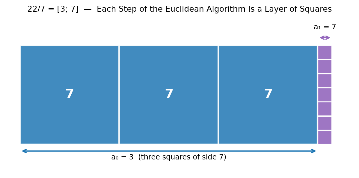
The Euclidean algorithm feels like abstract arithmetic — dividing, taking remainders, repeating. But every step is secretly a tiling: you pack the largest possible squares into a rectangle, and the remainder is the leftover strip. Let us make that geometry visible for 22/7.
```{python}
# uses: cf_rational()
#| label: fig-cfrac-euclidean
#| fig-cap: "The Euclidean algorithm as rectangle tiling: 22/7 = [3; 7]. Three 7×7 squares fill most of the 22×7 rectangle (a₀ = 3); seven 1×1 squares fill the leftover 1×7 strip (a₁ = 7)."
import matplotlib.pyplot as plt
import matplotlib.patches as patches

BLUE   = '#1f77b4'
PURPLE = '#9467bd'


fig, ax = plt.subplots(figsize=(9, 3.2))
for i in range(3):
    r = patches.FancyBboxPatch((i*7, 0), 6.95, 6.95, boxstyle="square,pad=0",
                               linewidth=1.2, edgecolor='white', facecolor=BLUE, alpha=0.85)
    ax.add_patch(r)
    ax.text(i*7+3.5, 3.5, '7', ha='center', va='center', color='white', fontsize=16, fontweight='bold')
for j in range(7):
    r = patches.FancyBboxPatch((21, j), 0.95, 0.95, boxstyle="square,pad=0",
                               linewidth=0.5, edgecolor='white', facecolor=PURPLE, alpha=0.9)
    ax.add_patch(r)
ax.annotate('', xy=(21, -0.5), xytext=(0, -0.5),
            arrowprops=dict(arrowstyle='<->', color=BLUE, lw=1.5))
ax.text(10.5, -1.1, 'a₀ = 3  (three squares of side 7)', ha='center', fontsize=9)
ax.annotate('', xy=(22, 7.5), xytext=(21, 7.5),
            arrowprops=dict(arrowstyle='<->', color=PURPLE, lw=1.5))
ax.text(21.5, 8.1, 'a₁ = 7', ha='center', fontsize=9)
ax.set_xlim(-1, 23.5); ax.set_ylim(-2.0, 9.0); ax.set_aspect('equal'); ax.axis('off')
ax.set_title('22/7 = [3; 7]  —  Each Step of the Euclidean Algorithm Is a Layer of Squares',
             fontsize=10, pad=6)
plt.tight_layout(); plt.show()
```
Three blue squares, seven purple squares — the whole algorithm drawn as geometry. Every coefficient is just "how many squares fit?" and you already know how to count squares.
Let us verify the first by hand: $22 = 3 \cdot 7 + 1$, so $a_0 = 3$.
Next, $7 = 7 \cdot 1 + 0$, so $a_1 = 7$ and we stop. Result: [3; 7].
For $\sqrt{D}$ (where $D$ is a positive integer that is not a perfect
square), an exact all-integer method avoids any floating-point
rounding. It tracks three integers $m_n, d_n, a_n$ and updates them by
$$m_{n+1} = d_n\, a_n - m_n, \qquad
d_{n+1} = \frac{D - m_{n+1}^2}{d_n}, \qquad
a_{n+1} = \left\lfloor\frac{a_0 + m_{n+1}}{d_{n+1}}\right\rfloor,$$
starting from $a_0 = \lfloor\sqrt{D}\rfloor$, $m_0 = 0$, $d_0 = 1$.
It can be shown by induction that $d_n$ always divides $D - m_{n+1}^2$
exactly, so every quantity stays an integer with no rounding at all.
```{python}
import math

def cf_sqrt(D, num_terms):
    """Exact integer CF coefficients for sqrt(D)."""
    a0 = math.isqrt(D)      # new: exact integer sqrt
    if a0 * a0 == D:
        return [a0]          # perfect square
    coeffs = [a0]
    m, d, a = 0, 1, a0
    for _ in range(num_terms - 1):
        m = d * a - m
        d = (D - m * m) // d
        a = (a0 + m) // d
        coeffs.append(a)
    return coeffs


# uses: cf_sqrt()
import math

for D in [2, 3, 5, 7, 13]:
    print(f"sqrt({D:2d}): {cf_sqrt(D, 12)}")
```
`math.isqrt(D)` (Python 3.8+) returns $\lfloor\sqrt{D}\rfloor$ using
integer arithmetic alone -- no floating-point approximation ever occurs.
The output reveals an immediate pattern: every non-square positive
integer $D$ produces a **repeating** block. We will examine why in
@sec-cfrac-periodic.
For arbitrary floating-point numbers, a simpler loop works for the
first ten or so coefficients before rounding errors accumulate:
```{python}
import math

def cf_float(x, max_terms=10):
    """Approximate CF from a float (loses precision after ~12 steps)."""
    coeffs = []
    for _ in range(max_terms):
        a = math.floor(x)
        coeffs.append(a)
        frac = x - a
        if frac < 1e-9:
            break
        x = 1.0 / frac
    return coeffs


# uses: cf_float()
import math

print("pi:", cf_float(math.pi, 8))
print("e: ", cf_float(math.e, 10))
```
The pi output [3, 7, 15, 1, 292, 1, 1, 1] matches the known values
exactly. The e output reveals a striking pattern:
[2, 1, 2, 1, 1, 4, 1, 1, 6, 1] -- every third term is an even number
that grows by 2. A transcendental number with such clean structure is
quite unusual; the full pattern is
$e = [2;\; 1, 2, 1, 1, 4, 1, 1, 6, 1, 1, 8, \ldots]$.
## Convergents: Best Rational Approximations {#sec-cfrac-convergents}
::: {.content-visible when-format="pdf"}
```{=latex}
\begin{center}
\begin{minipage}[c]{0.28\textwidth}\centering
\href{https://youtu.be/S0QtJ3kRezM}{\includegraphics[width=\textwidth]{images/thumb_S0QtJ3kRezM.jpg}}
\end{minipage}%
\hspace{0.02\textwidth}%
\begin{minipage}[c]{0.28\textwidth}
\small\textbf{MathsNeedNotApply}\\[3pt]
\small The Pi Approximation Tier List\\[3pt]
\small\href{https://youtu.be/S0QtJ3kRezM}{\texttt{youtu.be/S0QtJ3kRezM}}
\end{minipage}%
\hspace{0.02\textwidth}%
\begin{minipage}[c]{0.36\textwidth}
\small Ranks $\pi$ approximations from worst to best — showing why convergents from the continued fraction are provably the best possible rational approximations.
\end{minipage}
\end{center}
```
:::
::: {.content-visible when-format="html"}
<div style="display:flex; align-items:flex-start; margin:1em 0; gap:12px; width:100%;">
<div style="flex:0 0 200px;"><a href="https://youtu.be/S0QtJ3kRezM" target="_blank"><img src="https://img.youtube.com/vi/S0QtJ3kRezM/0.jpg" style="width:100%;" alt="The Pi Approximation Tier List"></a></div>
<div style="flex:1; font-size:0.85em;"><strong>MathsNeedNotApply</strong><br>The Pi Approximation Tier List<br><a href="https://youtu.be/S0QtJ3kRezM" target="_blank" style="font-family:monospace;">youtu.be/S0QtJ3kRezM</a></div>
<div style="flex:1; font-size:0.85em;">Ranks π approximations from worst to best — showing why convergents from the continued fraction are provably the best possible rational approximations.</div>
</div>
:::
Truncating a continued fraction at position $n$ gives a rational
approximation called the $n$-th **convergent**. The convergents of
$[a_0;\, a_1, a_2, \ldots]$ satisfy a two-step recurrence:
$$h_{-1} = 1, \quad h_0 = a_0, \quad
h_n = a_n\, h_{n-1} + h_{n-2}$$
$$k_{-1} = 0, \quad k_0 = 1, \quad
k_n = a_n\, k_{n-1} + k_{n-2}$$
The $n$-th convergent is $p_n/q_n = h_n/k_n$. Notice how similar this
is to the Fibonacci recurrence in @sec-fib-rabbits: when every
$a_n = 1$, the numerators and denominators are exactly the Fibonacci
numbers. We will return to this connection in @sec-cfrac-golden.
```{python}
# uses: cf_float()
from fractions import Fraction
import math

def convergents(coeffs):
    """Convergents of CF with given coefficients.
    Returns a list of Fraction objects (exact arithmetic)."""
    h_prev, h_curr = 1, coeffs[0]
    k_prev, k_curr = 0, 1
    result = [Fraction(h_curr, k_curr)]
    for a in coeffs[1:]:
        h_prev, h_curr = h_curr, a * h_curr + h_prev
        k_prev, k_curr = k_curr, a * k_curr + k_prev
        result.append(Fraction(h_curr, k_curr))
    return result


pi_cf = cf_float(math.pi, 7)      # [3, 7, 15, 1, 292, 1, 1]
pi_convs = convergents(pi_cf)
for c in pi_convs:
    err = abs(float(c) - math.pi)
    print(f"{str(c):13s} {float(c):.9f}  {err:.2e}")
```
`fractions.Fraction` is a Python standard-library class (no SymPy
needed) that stores a fraction as an exact ratio of two integers.
All arithmetic on `Fraction` objects is exact: `Fraction(1,3) +
Fraction(1,6)` gives `Fraction(1,2)`, never 0.4999..., which makes
it ideal for verifying convergent computations.
The convergents alternate above and below the true value:
$p_0/q_0 < \pi < p_1/q_1$, then $p_2/q_2 < \pi < p_3/q_3$, and so
on, closing in from both sides. The jump from $p_3/q_3 = 355/113$ to
$p_4/q_4 = 103993/33102$ is tiny in absolute error but requires a
denominator 300 times larger -- because the next coefficient is 292.
### Research Example: Do Convergents Alternate Above and Below $\pi$? {.unnumbered .unlisted}
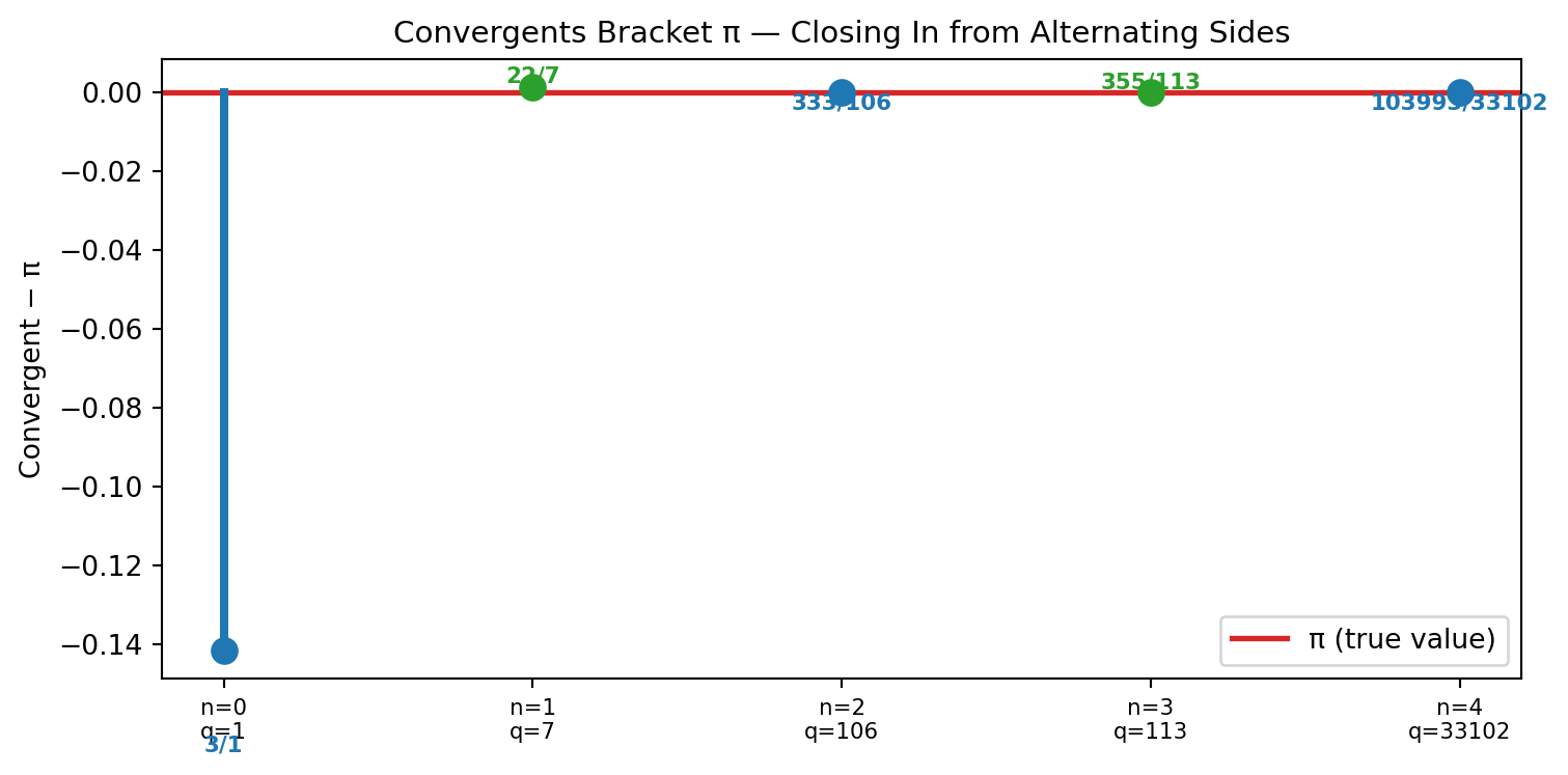
Each new convergent overshoots or undershoots π and then flips to the other side — they zero in from alternating directions. The gap between 355/113 and the next convergent should look absurdly small compared to the others. Let us check.
```{python}
# uses: convergents()
#| label: fig-cfrac-closeup
#| fig-cap: "Convergents of π alternate above (red) and below (blue) the true value. 355/113 sits so close that it takes a denominator 300× larger to improve on it."
import math
import matplotlib.pyplot as plt

RED   = '#d62728'
GREEN = '#2ca02c'
BLUE  = '#1f77b4'

labels_plot = ['3/1', '22/7', '333/106', '355/113', '103993/33102']
conv_vals = [3, 22/7, 333/106, 355/113, 103993/33102]
errors = [v - math.pi for v in conv_vals]
fig, ax = plt.subplots(figsize=(8, 4))
ax.axhline(0, color=RED, linewidth=2, label='π (true value)')
above_color, below_color = GREEN, BLUE
for i, (err, lbl) in enumerate(zip(errors, labels_plot)):
    c = above_color if err > 0 else below_color
    ax.plot([i, i], [0, err], color=c, linewidth=3)
    ax.plot(i, err, 'o', color=c, markersize=9)
    offset = abs(err) * 0.15
    ax.text(i, err + (offset if err > 0 else -offset), lbl, ha='center',
            va='bottom' if err > 0 else 'top', color=c, fontsize=8, fontweight='bold')
ax.set_xticks(range(5))
ax.set_xticklabels([f'n={i}\nq={[1,7,106,113,33102][i]}' for i in range(5)], fontsize=8)
ax.set_ylabel("Convergent − π")
ax.set_title("Convergents Bracket π — Closing In from Alternating Sides", fontsize=11)
ax.legend()
plt.tight_layout(); plt.show()
```
Red above, blue below — the alternation is exact, every time. And that near-zero bar at 355/113 shows why ancient astronomers used it for centuries: it is the last stop before the denominators explode. You found this with five lines of arithmetic.
More precisely, the convergents satisfy the **Best Approximation
Theorem** [@hardywright1979]: no fraction $p/q$ with $q \le q_n$ comes closer to
$\alpha$ than the $n$-th convergent $p_n/q_n$, except $p_n/q_n$
itself.
We can verify this computationally: search all fractions with
denominator at most 113 and confirm none beats 355/113.
```{python}
# uses: cf_float(), convergents()
import math
from fractions import Fraction

best_err = float('inf')
best_frac = None
for q in range(1, 114):
    p = round(math.pi * q)
    err = abs(p / q - math.pi)
    if err < best_err:
        best_err = err
        best_frac = Fraction(p, q)

print(f"Best approx (denom <= 113): {best_frac}")
print(f"Error:                      {best_err:.4e}")
ref = abs(355 / 113 - math.pi)
print(f"355/113 error:              {ref:.4e}")
```
The best rational approximation to $\pi$ with denominator at most 113
is indeed 355/113, confirming the theorem for this case.
## Quadratic Irrationals Are Periodic {#sec-cfrac-periodic}
```{python}
#| echo: false
from pathlib import Path; import urllib.request
_d = Path('images'); _d.mkdir(exist_ok=True)
_p = _d / 'lagrange.jpg'
if not _p.exists():
try:
req = urllib.request.Request(
'https://upload.wikimedia.org/wikipedia/commons/1/19/Joseph_Louis_Lagrange2.jpg',
headers={'User-Agent': 'Mozilla/5.0'})
with urllib.request.urlopen(req) as r:
_p.write_bytes(r.read())
except Exception: pass
```
::: {.content-visible when-format="pdf"}
```{=latex}
\begin{center}
\begin{minipage}[c]{0.22\textwidth}
\includegraphics[width=\textwidth]{images/lagrange.jpg}
\end{minipage}%
\hspace{0.03\textwidth}%
\begin{minipage}[c]{0.55\textwidth}
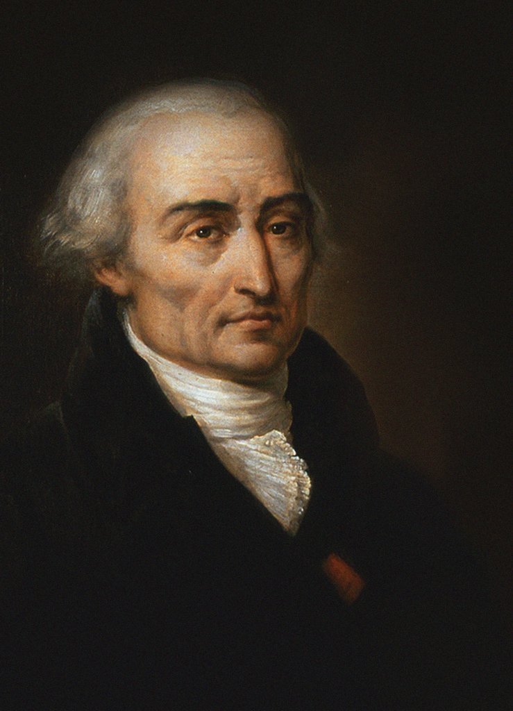
\small\textit{Joseph-Louis Lagrange (1736--1813)}\\[2pt]
\tiny Public domain, via Wikimedia Commons
\end{minipage}
\end{center}
```
:::
::: {.content-visible when-format="html"}
<div style="display:flex; align-items:center; margin:1em 0; gap:12px;">
<img src="images/lagrange.jpg" style="width:100px; flex-shrink:0;" alt="Joseph-Louis Lagrange">
<div style="font-size:0.82em;"><em>Joseph-Louis Lagrange (1736–1813)</em><br><span style="font-size:0.85em;">Public domain, via Wikimedia Commons</span></div>
</div>
:::
::: {.content-visible when-format="pdf"}
```{=latex}
\begin{center}
\begin{minipage}[c]{0.28\textwidth}\centering
\href{https://youtu.be/CaasbfdJdJg}{\includegraphics[width=\textwidth]{images/thumb_CaasbfdJdJg.jpg}}
\end{minipage}%
\hspace{0.02\textwidth}%
\begin{minipage}[c]{0.28\textwidth}
\small\textbf{Mathologer}\\[3pt]
\small Infinite fractions and the most irrational number\\[3pt]
\small\href{https://youtu.be/CaasbfdJdJg}{\texttt{youtu.be/CaasbfdJdJg}}
\end{minipage}%
\hspace{0.02\textwidth}%
\begin{minipage}[c]{0.36\textwidth}
\small Why the golden ratio is the ``most irrational'' number — its all-ones continued fraction makes every rational approximation as bad as possible.
\end{minipage}
\end{center}
```
:::
::: {.content-visible when-format="html"}
<div style="display:flex; align-items:flex-start; margin:1em 0; gap:12px; width:100%;">
<div style="flex:0 0 200px;"><a href="https://youtu.be/CaasbfdJdJg" target="_blank"><img src="https://img.youtube.com/vi/CaasbfdJdJg/0.jpg" style="width:100%;" alt="Infinite fractions and the most irrational number"></a></div>
<div style="flex:1; font-size:0.85em;"><strong>Mathologer</strong><br>Infinite fractions and the most irrational number<br><a href="https://youtu.be/CaasbfdJdJg" target="_blank" style="font-family:monospace;">youtu.be/CaasbfdJdJg</a></div>
<div style="flex:1; font-size:0.85em;">Why the golden ratio is the "most irrational" number — its all-ones continued fraction makes every rational approximation as bad as possible.</div>
</div>
:::
The `cf_sqrt` output showed that $\sqrt{2} = [1;\, \overline{2}]$,
$\sqrt{3} = [1;\, \overline{1, 2}]$, $\sqrt{5} = [2;\, \overline{4}]$
(the bar means the block repeats forever). Joseph-Louis Lagrange proved
in 1770 that a number has an eventually periodic continued fraction
**if and only if** it is a **quadratic irrational** -- the irrational
root of a quadratic equation $ax^2 + bx + c = 0$ with integer
coefficients [@lagrange1770; @hardywright1979, Thm. 177].
We detect the period by watching for a repeated $(m, d)$ state pair:
```{python}
import math

def cf_sqrt_period(D):
    """Return (a0, repeating_block) for the CF of sqrt(D)."""
    a0 = math.isqrt(D)
    if a0 * a0 == D:
        return (a0, [])
    seen = {}
    m, d, a = 0, 1, a0
    period = []
    while True:
        m = d * a - m
        d = (D - m * m) // d
        a = (a0 + m) // d
        state = (m, d)
        if state in seen:
            break
        seen[state] = len(period)
        period.append(a)
    return (a0, period)

# uses: cf_sqrt_period()
import math

print(f"{'D':>3}  CF representation         period")
print("-" * 42)
for D in [2, 3, 5, 6, 7, 10, 11, 13, 14]:
    a0, blk = cf_sqrt_period(D)
    cf_str = f"[{a0}; {blk}]"
    print(f"{D:3d}  {cf_str:25s}  {len(blk)}")
```
Notice that the repeating block always ends with $2a_0$ (twice the
integer part). This is a theorem, not a coincidence.
There is a classical connection to **Pell's equation**, which asks for
integer solutions to $x^2 - Dy^2 = \pm 1$. The numerator and
denominator of the last convergent before the period repeats always
give the smallest positive solution. For example, the convergents of
$\sqrt{2}$ are $1/1, 3/2, 7/5, 17/12, \ldots$, and indeed:
$1^2 - 2 \cdot 1^2 = -1$, $3^2 - 2 \cdot 2^2 = 1$,
$7^2 - 2 \cdot 5^2 = -1$, and so on, alternating $\pm 1$.
```{python}
# uses: cf_sqrt_period(), convergents()
import math

def pell_solutions(D, n_solutions=5):
    """First n Pell solutions x^2 - D*y^2 = +/- 1."""
    a0, blk = cf_sqrt_period(D)
    if not blk:
        return []
    # extend over several periods to get enough solutions
    full = [a0] + blk * (2 * n_solutions + 4)
    convs = convergents(full)
    results = []
    for c in convs:
        x, y = c.numerator, c.denominator
        val = x * x - D * y * y
        if abs(val) == 1:
            results.append((x, y, val))
            if len(results) >= n_solutions:
                break
    return results

# uses: pell_solutions()
import math

print("Pell solutions for D=2 (x^2 - 2y^2 = +/-1):")
for x, y, v in pell_solutions(2, 6):
    print(f"  {x}^2 - 2*{y}^2 = {v}")
```
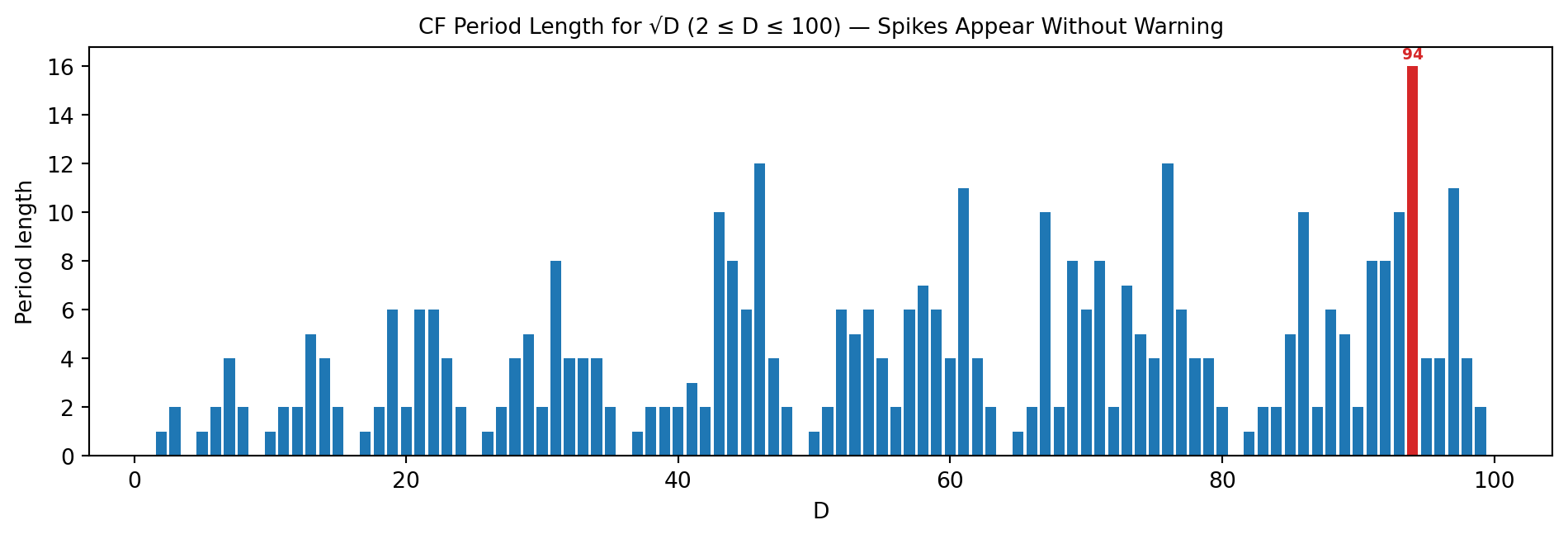
### Research Example: Which √D < 100 Has the Longest Continued-Fraction Period? {.unnumbered .unlisted}
Period length varies wildly from one D to the next — some square roots repeat after just one coefficient, others take many more. Is there a pattern? Let us compute the period length for every non-square D from 2 to 100 and look for the record-holders.
```{python}
#| label: fig-cfrac-periods
#| fig-cap: "CF period lengths for √D, non-square D from 2 to 100. Most periods are short; a handful of D values stand out with the longest period — including the famous D = 61 whose Pell equation solution exceeds a billion."
# uses: cf_sqrt_period()
import math
import matplotlib.pyplot as plt

BLUE = '#1f77b4'
RED  = '#d62728'

ds      = [d for d in range(2, 101) if math.isqrt(d)**2 != d]
periods = [len(cf_sqrt_period(d)[1]) for d in ds]
max_p   = max(periods)

fig, ax = plt.subplots(figsize=(10, 3.5))
colors = [RED if p == max_p else BLUE for p in periods]
ax.bar(ds, periods, color=colors, width=0.8, edgecolor='none')
for d, p in zip(ds, periods):
    if p == max_p:
        ax.text(d, p + 0.15, str(d), ha='center', va='bottom',
                fontsize=7, color=RED, fontweight='bold')
ax.set_xlabel("D")
ax.set_ylabel("Period length")
ax.set_title("CF Period Length for √D (2 ≤ D ≤ 100) — Spikes Appear Without Warning",
             fontsize=10)
plt.tight_layout()
plt.show()
```
The bars spike and dip without an obvious formula — yet every value is exact and provable. The red bar at D = 61 is the record-holder: its Pell equation $x^2 - 61y^2 = 1$ has smallest solution $x = 1{,}766{,}319{,}049$, a number that Indian mathematician Brahmagupta effectively found in the 7th century [@hardywright1979] — long before Pell was born.
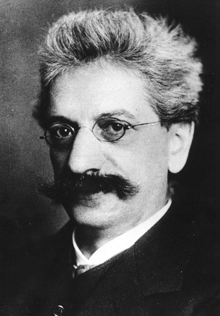
## The Golden Ratio: Hardest to Approximate {#sec-cfrac-golden}
```{python}
#| echo: false
from pathlib import Path; import urllib.request
_d = Path('images'); _d.mkdir(exist_ok=True)
_p = _d / 'hurwitz.jpg'
if not _p.exists():
try:
req = urllib.request.Request(
'https://upload.wikimedia.org/wikipedia/commons/3/3a/Adolf_Hurwitz_1910s.jpg',
headers={'User-Agent': 'Mozilla/5.0'})
with urllib.request.urlopen(req) as r:
_p.write_bytes(r.read())
except Exception: pass
```
::: {.content-visible when-format="pdf"}
```{=latex}
\begin{center}
\begin{minipage}[c]{0.22\textwidth}
\includegraphics[width=\textwidth]{images/hurwitz.jpg}
\end{minipage}%
\hspace{0.03\textwidth}%
\begin{minipage}[c]{0.55\textwidth}
\small\textit{Adolf Hurwitz (1859--1919)}\\[2pt]
\tiny Public domain, Mondadori Publishers, via Wikimedia Commons
\end{minipage}
\end{center}
```
:::
::: {.content-visible when-format="html"}
<div style="display:flex; align-items:center; margin:1em 0; gap:12px;">
<img src="images/hurwitz.jpg" style="width:100px; flex-shrink:0;" alt="Adolf Hurwitz">
<div style="font-size:0.82em;"><em>Adolf Hurwitz (1859–1919)</em><br><span style="font-size:0.85em;">Public domain, Mondadori Publishers, via Wikimedia Commons</span></div>
</div>
:::
::: {.content-visible when-format="pdf"}
```{=latex}
\begin{center}
\begin{minipage}[c]{0.28\textwidth}\centering
\href{https://youtu.be/sj8Sg8qnjOg}{\includegraphics[width=\textwidth]{images/thumb_sj8Sg8qnjOg.jpg}}
\end{minipage}%
\hspace{0.02\textwidth}%
\begin{minipage}[c]{0.28\textwidth}
\small\textbf{Numberphile}\\[3pt]
\small The Golden Ratio (why it is so irrational)\\[3pt]
\small\href{https://youtu.be/sj8Sg8qnjOg}{\texttt{youtu.be/sj8Sg8qnjOg}}
\end{minipage}%
\hspace{0.02\textwidth}%
\begin{minipage}[c]{0.36\textwidth}
\small The golden ratio's continued fraction $[1; 1, 1, 1, \ldots]$ makes it the hardest number to approximate with fractions — visualized with rotating sunflower spirals.
\end{minipage}
\end{center}
```
:::
::: {.content-visible when-format="html"}
<div style="display:flex; align-items:flex-start; margin:1em 0; gap:12px; width:100%;">
<div style="flex:0 0 200px;"><a href="https://youtu.be/sj8Sg8qnjOg" target="_blank"><img src="https://img.youtube.com/vi/sj8Sg8qnjOg/0.jpg" style="width:100%;" alt="The Golden Ratio (why it is so irrational)"></a></div>
<div style="flex:1; font-size:0.85em;"><strong>Numberphile</strong><br>The Golden Ratio (why it is so irrational)<br><a href="https://youtu.be/sj8Sg8qnjOg" target="_blank" style="font-family:monospace;">youtu.be/sj8Sg8qnjOg</a></div>
<div style="flex:1; font-size:0.85em;">The golden ratio's continued fraction [1; 1, 1, 1, …] makes it the hardest number to approximate with fractions — visualized with rotating sunflower spirals.</div>
</div>
:::
In @sec-fib-golden we met the golden ratio $\varphi = (1+\sqrt{5})/2$.
Its continued fraction is the simplest possible infinite sequence:
$\varphi = [1;\, 1, 1, 1, \ldots]$ -- all ones, forever.
```{python}
# uses: cf_float()
import math

phi_approx = (1 + math.sqrt(5)) / 2
print("phi (float):", cf_float(phi_approx, 14))
```
Because every partial quotient is 1, the convergents grow as slowly
as possible. Computing them with exact arithmetic confirms the
Fibonacci connection noted in @sec-fib-golden:
```{python}
# uses: convergents()
import math

# Phi = [1; 1, 1, 1, ...], 16 terms exactly
phi_convs = convergents([1] * 16)
print("Phi convergents (numerator/denominator):")
for c in phi_convs[:10]:
    print(f"  {c.numerator}/{c.denominator}")
```
The numerators and denominators are consecutive Fibonacci numbers:
$1/1, 2/1, 3/2, 5/3, 8/5, 13/8, \ldots$ The ratio $F(n+1)/F(n)$
converges to $\varphi$ from alternating sides, just as we saw in
@sec-fib-rabbits.
Because $\varphi$ has all-1 partial quotients, no fraction with a
given denominator can approximate it substantially better than the
corresponding Fibonacci ratio. This is the content of
**Hurwitz's theorem** [@hurwitz1891]: for any irrational $\alpha$, the
inequality
$$\left|\alpha - \frac{p}{q}\right| < \frac{1}{\sqrt{5}\, q^2}$$
holds for infinitely many fractions $p/q$. For the golden ratio, the
constant $\sqrt{5}$ in the denominator cannot be replaced by anything
larger: $\varphi$ is the **hardest real number to approximate by
rationals**.
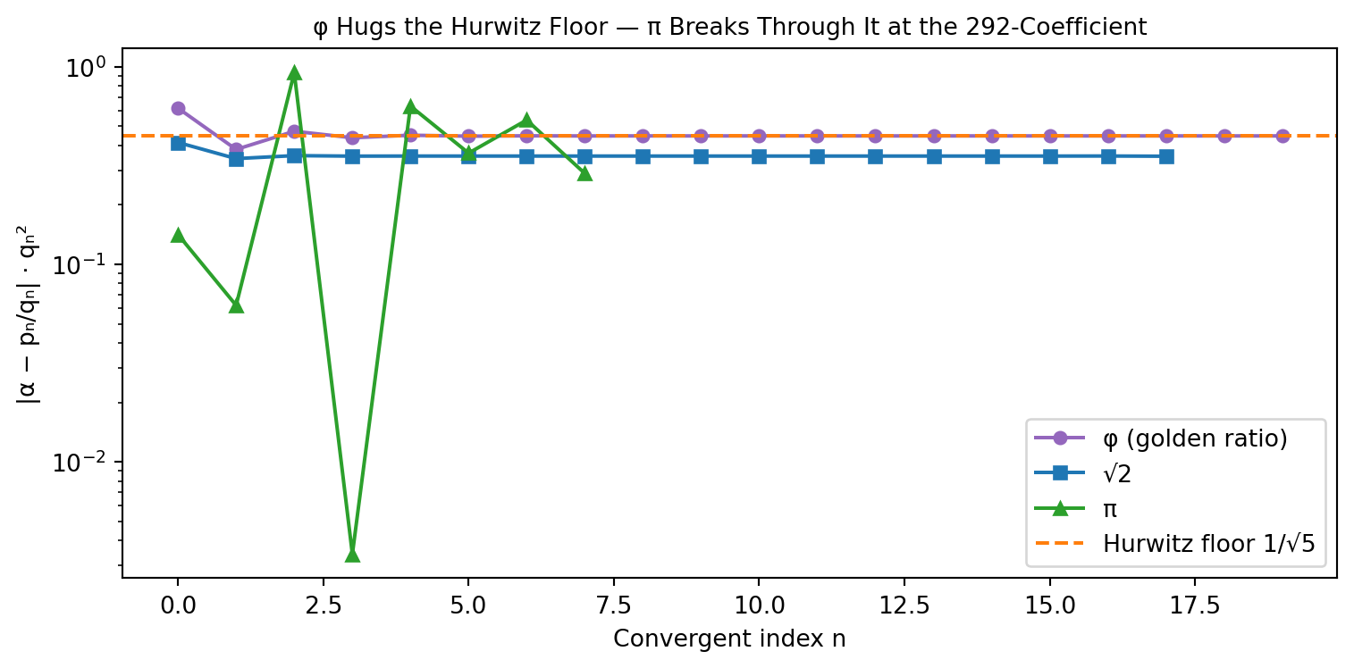
We can visualize this by plotting the scaled approximation error
$|\alpha - p_n/q_n| \cdot q_n^2$ for the convergents of several
numbers. For $\varphi$ this quantity should hover right at
$1/\sqrt{5} \approx 0.447$; for $\pi$ it should plunge far below that
floor near the 292-coefficient convergent.
### Research Example: Does $\varphi$ Really Hug the Hardest-to-Approximate Boundary? {.unnumbered .unlisted}
Hurwitz's theorem says every irrational can be approximated within $1/(\sqrt{5}\,q^2)$ infinitely often, and φ is the extreme case — it hugs that floor and never dips below. We can see this directly by plotting the scaled error $|\alpha - p_n/q_n| \cdot q_n^2$ for φ, √2, and π side by side.
```{python}
#| label: fig-cfrac-quality
#| fig-cap: "Scaled approximation error for φ (circles), √2 (squares), and π (triangles). φ hovers right at the Hurwitz floor 1/√5 ≈ 0.447; π plunges far below at index 4 — the 292 miracle."
# uses: convergents(), cf_sqrt(), cf_float()
import math
import matplotlib.pyplot as plt

BLUE   = '#1f77b4'
ORANGE = '#ff7f0e'
GREEN  = '#2ca02c'
PURPLE = '#9467bd'

# phi: exact all-1 CF, value approximated from float
phi_val = (1 + math.sqrt(5)) / 2
phi_convs_all = convergents([1] * 20)
phi_errs = [abs(float(c) - phi_val) * c.denominator**2
            for c in phi_convs_all]

# sqrt(2): exact integer CF
s2_convs = convergents(cf_sqrt(2, 18))
s2_val = math.sqrt(2)
s2_errs = [abs(float(c) - s2_val) * c.denominator**2
           for c in s2_convs]

# pi: float CF (accurate for first 8 terms)
pi_convs_all = convergents(cf_float(math.pi, 8))
pi_errs = [abs(float(c) - math.pi) * c.denominator**2
           for c in pi_convs_all]

fig, ax = plt.subplots(figsize=(8, 4))
ax.plot(phi_errs, marker='o', markersize=5, color=PURPLE, linewidth=1.5, label='φ (golden ratio)')
ax.plot(s2_errs,  marker='s', markersize=5, color=BLUE,   linewidth=1.5, label='√2')
ax.plot(pi_errs,  marker='^', markersize=5, color=GREEN,  linewidth=1.5, label='π')
ax.axhline(1 / math.sqrt(5), color=ORANGE, linestyle='--', linewidth=1.5, label='Hurwitz floor 1/√5')
ax.set_yscale('log')
ax.set_xlabel("Convergent index n")
ax.set_ylabel("|α − pₙ/qₙ| · qₙ²")
ax.set_title("φ Hugs the Hurwitz Floor — π Breaks Through It at the 292-Coefficient", fontsize=10)
ax.legend()
plt.tight_layout()
plt.show()
```
φ hugging the green dashed floor while π crashes through it at index 4 — that single dip is the geometric signature of the 292 coefficient. You just reproduced a result from analytic number theory with a for-loop and a plot.
## The Gauss-Kuzmin Distribution {#sec-cfrac-gauss-kuzmin}
Pick a "random" real number and compute its continued fraction. What
fraction of the partial quotients equal 1? Equal 2? Equal 7?
Karl Friedrich Gauss noticed around 1800 that the partial quotients
follow a definite probability distribution. This was proved rigorously
by Rodion Kuzmin in 1928 and independently by Paul Lévy in 1929 [@kuzmin1928; @levy1929]:
$$P(a = k) = \log_2\!\left(\frac{(k+1)^2}{k(k+2)}\right)
= \log_2\!\left(1 + \frac{1}{k(k+2)}\right).$$
Here $\log_2$ means logarithm base 2 (introduced in
@sec-pascal-dimension). The probabilities for small $k$:
| $k$ | Formula | Probability |
|-----|---------|-------------|
| 1 | $\log_2(4/3)$ | 41.5% |
| 2 | $\log_2(9/8)$ | 17.0% |
| 3 | $\log_2(16/15)$ | 9.3% |
| 4 | $\log_2(25/24)$ | 5.9% |
| 5 | $\log_2(36/35)$ | 4.1% |
Small partial quotients dominate overwhelmingly. The coefficient 1
appears in more than two of every five positions. A telescoping
product argument shows that the probabilities sum exactly to 1.
Let us verify this experimentally. The key tool is the **Gauss map**
$T(x) = \{1/x\}$ (the fractional part of $1/x$). Applying $T$
repeatedly to any $x \in (0, 1)$ produces one partial quotient at each
step and maps the interval back into $(0, 1)$, so the iteration
continues indefinitely.
### Research Example: Does Partial Quotient 1 Really Appear 41% of the Time? {.unnumbered .unlisted}
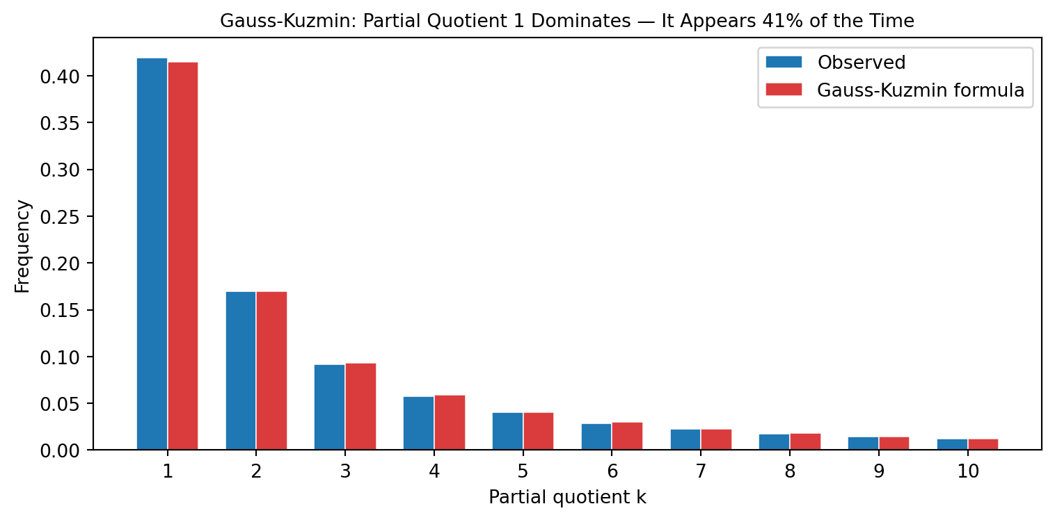
Gauss conjectured, and Kuzmin proved, that the partial quotients of a random real number follow a precise distribution: coefficient 1 appears about 41% of the time, coefficient 2 about 17%, and so on. Let us generate 3000 random numbers, apply the Gauss map, and see whether the counts match the formula.
```{python}
#| label: fig-cfrac-gkdist
#| fig-cap: "Observed partial-quotient frequencies (blue) match the Gauss-Kuzmin formula (orange) closely. Coefficient 1 wins by a landslide at 41%."
import math
import random
import matplotlib.pyplot as plt

BLUE = '#1f77b4'
RED  = '#d62728'

random.seed(42)
counts = {}
n_total = 0
for _ in range(3000):
    x = random.random()        # uniform in (0, 1)
    for _ in range(40):        # apply Gauss map 40 times
        if x < 1e-10:
            break
        x = 1.0 / x            # reciprocal
        a = math.floor(x)      # partial quotient
        x -= a                 # fractional part (back in (0,1))
        counts[a] = counts.get(a, 0) + 1
        n_total += 1

def gk_prob(k):
    return math.log((k + 1)**2 / (k * (k + 2)), 2)

ks = list(range(1, 11))
observed    = [counts.get(k, 0) / n_total for k in ks]
theoretical = [gk_prob(k)                 for k in ks]

fig, ax = plt.subplots(figsize=(8, 4))
width = 0.35
xs = range(len(ks))
ax.bar([x - width / 2 for x in xs], observed,
       width, label='Observed', color=BLUE, edgecolor='white', linewidth=0.6)
ax.bar([x + width / 2 for x in xs], theoretical,
       width, label='Gauss-Kuzmin formula', color=RED, alpha=0.9,
       edgecolor='white', linewidth=0.6)
ax.set_xticks(list(xs))
ax.set_xticklabels([str(k) for k in ks])
ax.set_xlabel("Partial quotient k")
ax.set_ylabel("Frequency")
ax.set_title("Gauss-Kuzmin: Partial Quotient 1 Dominates — It Appears 41% of the Time",
             fontsize=10)
ax.legend()
plt.tight_layout()
plt.show()
```
Blue and orange bars almost indistinguishable — Gauss's two-century-old conjecture confirmed in seconds by a random simulation. The 1800s had to wait for Kuzmin's proof; you just watched it happen with three dozen lines of Python.
The Gauss-Kuzmin distribution has two elegant corollaries.
**Lévy's constant.** The denominator $q_n$ of the $n$-th convergent
grows on average like $e^{n\beta}$ where
$\beta = \pi^2/(12 \ln 2) \approx 1.1865$. That is, for almost every
irrational $\alpha$, we have $q_n^{1/n} \to e^\beta \approx 3.276$
as $n \to \infty$.
### Research Example: Do Convergent Denominators Really Grow Like $e^{n\beta}$? {.unnumbered .unlisted}
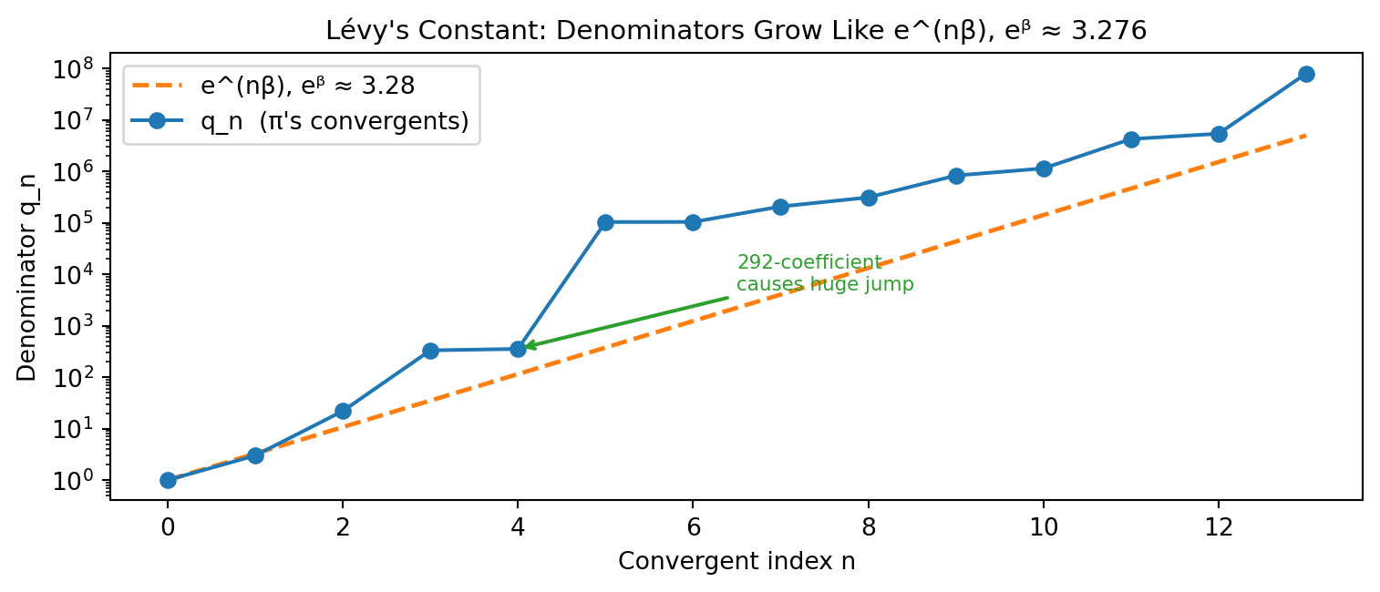
Lévy proved that for almost every irrational number the convergent denominators $q_n$ grow exponentially at rate $e^\beta$ where $\beta = \pi^2/(12\ln 2) \approx 1.187$. Let us check whether π's denominators actually follow this curve — and watch what the 292 coefficient does to the trend.
```{python}
#| label: fig-cfrac-levy
#| fig-cap: "Denominator growth for π's convergents (blue) vs. Lévy's exponential trend e^(nβ) (dashed orange). The 292-coefficient causes a dramatic jump at n = 4."
import math
import matplotlib.pyplot as plt

BLUE   = '#1f77b4'
ORANGE = '#ff7f0e'
GREEN  = '#2ca02c'

beta = math.pi**2 / (12 * math.log(2))
e_beta = math.exp(beta)
pi_cf_long = [3, 7, 15, 1, 292, 1, 1, 1, 2, 1, 3, 1, 14]
qs = [1]; k_p, k_c = 0, 1
for a in pi_cf_long:
    k_p, k_c = k_c, a * k_c + k_p; qs.append(k_c)
ns = list(range(len(qs)))
fig, ax = plt.subplots(figsize=(8, 3.5))
levy_y = [e_beta**n for n in ns]
ax.semilogy(ns, levy_y, '--', color=ORANGE, linewidth=1.8, label=f'e^(nβ), eᵝ ≈ {e_beta:.2f}')
ax.semilogy(ns, qs, 'o-', color=BLUE, markersize=6, linewidth=1.5, label="q_n  (π's convergents)")
ax.annotate('292-coefficient\ncauses huge jump', xy=(4, qs[4]), xytext=(6.5, 5000),
            arrowprops=dict(arrowstyle='->', color=GREEN, lw=1.5), color=GREEN, fontsize=8)
ax.set_xlabel("Convergent index n")
ax.set_ylabel("Denominator q_n")
ax.set_title(f"Lévy's Constant: Denominators Grow Like e^(nβ), eᵝ ≈ {e_beta:.3f}", fontsize=11)
ax.legend()
plt.tight_layout(); plt.show()
```
The blue dots track the orange trend almost perfectly — then the 292 coefficient fires and the denominator rockets upward in one step. Lévy's constant, proved in 1929, jumps off the page as a single annotated spike. You needed only a list, a loop, and a semilogy call.
**Coprime probability.** The probability that two randomly chosen
positive integers have no common factor is
$6/\pi^2 \approx 60.8\%$ [@hardywright1979, Thm. 332].
This connects the geometry of circles ($\pi$) to the arithmetic of
primes through the Riemann zeta function at $s = 2$. (We will meet
this connection again in Chapter 9.)
```{python}
import random
import math

random.seed(0)
n_coprime = sum(
    1 for _ in range(100000)
    if math.gcd(
        random.randint(1, 10**6),
        random.randint(1, 10**6)
    ) == 1
)
frac = n_coprime / 100000
print(f"Observed coprime fraction: {frac:.4f}")
print(f"6/pi^2 =                   {6/math.pi**2:.4f}")
```
`math.gcd` was introduced in @sec-fib-identities. Here it is doing
double duty: running 100,000 GCD computations in a loop is fast enough
to confirm the theoretical value to three decimal places.
## Further Research Topics {#sec-cfrac-research}
1. **The Pell equation survey.** For each non-square $D$ from 2 to 20,
use `cf_sqrt_period` and `convergents` to find the smallest positive
integers $x, y$ satisfying $x^2 - Dy^2 = 1$. Record the solution
and the period length for each $D$. Which $D$ in this range
produces the largest fundamental solution? (Hint: try $D = 13$.)
For a harder challenge, extend to $D \le 100$ and verify that
$D = 61$ gives $x = 1766319049$, $y = 226153980$.
*(Problem proposed by Claude Code.)*
2. **The pattern in $e$.** Compute the first 30 partial quotients of
$e = 2.71828\ldots$ (use known values if your float loses precision).
Confirm or challenge the conjecture
$e = [2;\; 1, 2, 1, 1, 4, 1, 1, 6, 1, 1, 8, \ldots]$ where every
third term increments by 2. Can you write a formula for the $n$-th
partial quotient? Search the OEIS for the sequence of partial
quotients (see Chapter 8).
*(Problem proposed by Claude Code.)*
3. **Coprime probability as a function of scale.** Modify the coprime
experiment to count pairs $(p, q)$ with $1 \le p, q \le N$ for
$N = 10, 100, 1000, 10000$. Plot the observed fraction vs $N$ on a
log scale and compare with the horizontal line at $6/\pi^2$. At
what $N$ does the approximation stabilize to within 1%?
*(Problem proposed by Claude Code.)*
4. **Convergent accuracy race.** For $\sqrt{2}$, $\sqrt{3}$, $\sqrt{5}$,
and $\pi$, plot the number of correct decimal digits delivered by
the $n$-th convergent as a function of $n$. Which number gives the
slowest convergence per convergent? Which gives the fastest? Connect
your answer to the size of the typical partial quotients.
*(Problem proposed by Claude Code.)*
5. **Large-coefficient treasure hunt.** A partial quotient much larger
than its neighbors signals an unusually close rational approximation.
Compute the first 30 CF coefficients of each of $\pi, e, \sqrt{2},
\ln 2, \sqrt[3]{2}$, and the golden ratio. Report the largest
coefficient found for each number and the fraction it produces.
Which number has the most "surprising" near-rational value?
*(Problem proposed by Claude Code.)*
6. **Verifying Lévy's constant** [@levy1929]**.** Pick any irrational of your choice
(e.g., $\sqrt{7}$) and compute its first 50 convergents. For each
$n$, compute $q_n^{1/n}$ where $q_n$ is the denominator of the
$n$-th convergent. Does the sequence appear to stabilize? To what
value? Compare with $e^{\pi^2/(12 \ln 2)} \approx 3.2758$.
*(Problem proposed by Claude Code.)*
7. **Three-distance theorem.** Place $N$ points at positions
$\lfloor n\alpha \rfloor \bmod 1$ on the interval $[0, 1)$ for
$n = 1, 2, \ldots, N$ and any irrational $\alpha$. A theorem proved by
Vera Sós in 1958 [@sos1958] (conjectured by Steinhaus) says the $N$ points
divide $[0,1)$ into gaps of at most three distinct lengths, and the gap
sizes are controlled by the CF of $\alpha$. Verify this computationally for
$\alpha = \sqrt{2}$ and $N = 5, 8, 13, 21, 34$ (the Fibonacci
numbers). How do the gap sizes change at each Fibonacci step?
*(Problem proposed by Claude Code.)*
8. **Beyond quadratic: CF of $\sqrt[3]{2}$.** Compute the CF of
$\sqrt[3]{2} \approx 1.2599$ to 40 terms using `cf_float` (or a
high-precision library). Does the sequence appear periodic? By
Lagrange's theorem [@lagrange1770] it should not -- only quadratic irrationals
are periodic. Is the CF of $\sqrt[3]{2}$ well-known? Search OEIS
for the sequence of partial quoticients.
*(Problem proposed by Claude Code.)*
9. **Gauss-Kuzmin chi-squared test.** Repeat the Gauss-Kuzmin
experiment with 50,000 starting points instead of 3,000. Compute
the chi-squared statistic
$\chi^2 = \sum_{k=1}^{10} (O_k - E_k)^2 / E_k$
where $O_k$ and $E_k$ are the observed and expected counts.
A value below 16.9 indicates the match is within the 95% confidence
threshold for 9 degrees of freedom. At what sample size do you
first achieve $\chi^2 < 10$?
*(Problem proposed by Claude Code.)*
10. **Best approximation theorem verification.** The theorem states that
no fraction $p/q$ with $q \le q_n$ approximates $\alpha$ better
than the convergent $p_n/q_n$. Write a brute-force search that
checks all fractions with denominator at most $q_n$ for a specific
irrational $\alpha$ and confirms that the convergent wins. Test it
for $\alpha = \sqrt{3}$ and the first six convergents.
*(Problem proposed by Claude Code.)*
11. **Gosper's continued fraction arithmetic.** Bill Gosper invented an
algorithm for adding, multiplying, and taking square roots of
continued fractions directly -- without ever converting to decimal.
Look up Gosper's 1972 paper [@gosper1972] (or a modern exposition) and implement
`cf_add(cf1, cf2)` that takes two CF coefficient lists and returns
the CF of their sum. Test it on $\sqrt{2} + 1$, which should give
$[2;\, \overline{2}]$.
*(Problem proposed by Claude Code.)*
12. **Identifying mystery constants.** Use SymPy's `nsimplify` function
(or look ahead to Chapter 8) to try to identify the following
"mystery numbers" from their continued fractions:
(a) $[0;\, 3, 4, 3, 1, 3, 1, 8, \ldots]$ (first 20 terms);
(b) the constant whose CF is $[1;\, 1, 2, 1, 1, 4, 1, 1, 6, \ldots]$
(one-half of something familiar?);
(c) the positive root of $x^2 = x + 1$ (which you already know --
verify by CF). Can you reverse-engineer a number from its
partial-quotient fingerprint alone?
*(Problem proposed by Claude Code.)*
13. **Calendar design by continued fractions.** The true solar year is
approximately 365.24219 days, so the fractional part is
$f \approx 0.24219$. Compute the CF of $f$ with `cf_float` and find
its first several convergents. The Julian calendar uses $1/4$: add a
leap day every four years. The Gregorian calendar uses $97/400$:
skip three leap years every 400 years. Verify in Python which
convergent is closer to the true value. What does the *next*
convergent after $97/400$ suggest? How many years long would a
calendar based on that convergent be, and by how many seconds per
year would it still drift? This is a perfect example of deliberately
choosing a "good enough" approximation over the best one because the
denominator fits a human-scale calendar.
*(Problem proposed by Claude Code.)*
14. **Music and the twelfth root of 2.** A perfect fifth sounds pleasing
because two pitches at a $3:2$ frequency ratio have overlapping
overtones. For twelve-tone equal temperament to include a near-perfect
fifth, we need $2^{7/12} \approx 3/2$, which means $7/12$ must be a
good rational approximation to $\log_2 3 - 1$. Compute the CF of
$\log_2 3$ and find its convergents. Show that the denominators
$1, 2, 5, 12, 41, 53, 306, \ldots$ each give an equal-division scale
where the "closest fifth" is especially accurate. For each denominator
$n$ in that list, compute the error $|2^{k/n} - 3/2|$ where $k$ is
the numerator of the corresponding convergent. Plot this error vs.\ $n$
on a log scale. Why does 12 win in practice even though 53 is
mathematically better?
*(Problem proposed by Claude Code.)*
15. **Lamé's theorem and the Fibonacci worst case.** In 1844 Édouard Lamé
proved [@lame1844] that the number of steps of the Euclidean algorithm on inputs
$(a, b)$ with $b \le n$ never exceeds $\log_\varphi(n\sqrt{5})$.
The worst-case pair is always consecutive Fibonacci numbers.
Verify this experimentally: for each $k$ from 2 to 30, apply the
Euclidean algorithm to $(F_{k+1}, F_k)$ and count the division steps.
Plot steps vs.\ $k$ and confirm the growth looks like
$k \cdot \log \varphi$. Then write a brute-force search: for each
$n$ from 2 to 200, find the pair $(a, b)$ with $a, b \le n$ that
maximizes the step count. Is the winner always a pair of consecutive
Fibonacci numbers? If not, what is it?
*(Problem proposed by Claude Code.)*
16. **Khinchin's constant** [@khinchin1964]**.** One of the strangest theorems in analysis says
that for almost every real number $x$ (exceptions have probability
zero), the geometric mean of the first $n$ partial quotients converges
to the same constant $K \approx 2.6854520010\ldots$ regardless of
which $x$ you pick. Compute the first 80 partial quotients of
$\sqrt{2}, \sqrt{3}, \sqrt{5}, \sqrt{7}, \pi, e, \ln 2$, and five
random decimals. For each, plot the geometric mean after $k$ terms as
$k$ goes from 5 to 80. Do the random decimals converge toward $K$?
What about $\sqrt{2}$ and $\varphi$? (They are exceptional cases ---
why?) At what $k$ do the non-exceptional numbers first come within
$0.01$ of $K$?
*(Problem proposed by Claude Code.)*
17. **The Stern-Brocot tree** [@stern1858]**.** Build the fraction $3/5$ by starting
with neighbors $0/1$ and $1/0$ and repeatedly taking the
*mediant* $(a+c)/(b+d)$ of the two nearest bounding fractions.
The left/right choices you make form a binary sequence. Now encode
the CF of $3/5$ as a binary sequence: $a_1$ steps left, $a_2$
steps right, $a_3$ steps left, \ldots Verify that the two sequences
are identical. Then implement `stern_brocot_path(p, q)` that finds
any rational $p/q$ and returns its path. Use the path to prove
algorithmically that every positive rational appears in the tree
exactly once. As an extension, navigate to an irrational such as
$\sqrt{2} - 1$ by truncating at 20 levels and see which fraction
the tree settles on.
*(Problem proposed by Claude Code.)*
18. **Hurwitz's theorem: how well can you approximate an irrational?**
Hurwitz proved [@hurwitz1891] that for any irrational $\alpha$ there are infinitely
many rationals $p/q$ satisfying $|\alpha - p/q| < 1/(\sqrt{5}\,q^2)$,
and $\sqrt{5}$ is the sharpest possible constant (it cannot be
increased for every irrational). Write code that, for a given $\alpha$,
finds all convergents $p_n/q_n$ with $q_n \le 500$ and plots the
quantity $C_n = 1/(q_n^2\,|\alpha - p_n/q_n|)$. Run it for
$\varphi$, $\sqrt{2}$, $\sqrt{3}$, $e$, and $\pi$. For which number
does $C_n$ always stay below $\sqrt{5}$? For which numbers does it
appear to approach a larger constant? From your data, can you guess
the analogous "best constant" for $\sqrt{2}$?
*(Problem proposed by Claude Code.)*
19. **Markov numbers and Markov triples.** The *Markov equation* is
$x^2 + y^2 + z^2 = 3xyz$. Its positive-integer solutions are called
Markov triples, and the largest element in each triple is a Markov
number: $1, 2, 5, 13, 29, 34, 89, 169, 194, \ldots$ Starting from
the root triple $(1, 1, 1)$, any triple $(a, b, c)$ generates three
new triples by "flipping" one element: if you replace $c$ with
$c' = 3ab - c$, you get another solution. Write a BFS or DFS that
generates all Markov triples with max element $\le 1000$ and count
them. Can you find two different triples that share the same largest
element? (The *Markov uniqueness conjecture* [@markov1879], unsolved since 1879,
says no such pair exists.) For a deeper dive, look up how Markov
numbers connect to the Lagrange spectrum of best-approximation
constants.
*(Problem proposed by Claude Code.)*
20. **Minkowski's question-mark function** [@minkowski1904]**.** Define $?(x)$ for
$x = [0;\, a_1, a_2, a_3, \ldots]$ by
$$?(x) \;=\; 2\sum_{i=1}^{\infty}(-1)^{i+1}\,2^{-(a_1+a_2+\cdots+a_i)}.$$
Implement this formula and plot $?(x)$ for $x \in [0, 1]$ using
200 sample points. The graph looks like a staircase that is
continuous and strictly increasing yet has zero derivative almost
everywhere --- a "devil's staircase." Verify numerically:
$?(1/2) = 1/2$; $?(\varphi - 1) = 2/3$ where $\varphi$ is the
golden ratio; and the image of every quadratic irrational under $?$
appears to be rational. Test this last claim on $\sqrt{2}-1$,
$\sqrt{3}-1$, and $(\sqrt{5}-1)/2$. What rational does each map to?
Can you prove it from the CF definition of $?$?
*(Problem proposed by Claude Code.)*