# Random Walks: Wandering with Purpose {#sec-walks}
## A Drunk's Journey Home {#sec-walks-intro}
Imagine a street stretching to infinity in both directions.
A person stands at position zero and begins walking.
Every second they take exactly one step, but they cannot
control the direction: left or right is equally likely.
After ten minutes (600 steps), where are they likely to be?
After one thousand steps?
Will they ever come back to where they started?
These are the core questions of the
**one-dimensional random walk**.
The model looks too simple to be interesting, but the same
mathematics governs some of the most important processes in
science [@pearson1905].
A molecule in a gas bounces off neighbors at each collision;
its path is a random walk in three dimensions.
A stock price drifts up and down with each trade.
The path of a foraging bee through a flower meadow is a
random walk in two dimensions.
Each of these looks chaotic in the small, yet perfectly
regular patterns emerge when we zoom out -- and those
patterns begin with the simple coin-flip model below.
The number line is the game board.
The walker starts at position 0.
At each step they move to position $+1$ or $-1$ with
equal probability $\frac{1}{2}$.
The first ten steps are short enough to follow by hand.
```{python}
import random

random.seed(42)
pos = 0
for step in range(1, 11):
    move = random.choice([-1, 1])
    pos += move
    dr = "right" if move == 1 else "left"
    print(f"Step {step:2}: {dr:5}  pos = {pos:3}")
```
The walker hits zero at step 6 and again at step 8.
In @sec-walks-return we will see that roughly half of all
walks return to zero within just two steps -- a fact that
surprises almost everyone when they first encounter it.
---
## Simulating a 1D Walk in Python {#sec-walks-1d}
Ten steps by hand is instructive; ten thousand require
automation.
NumPy, first introduced in @sec-fractals-mandelbrot,
provides a function `np.cumsum` that converts a list of
steps into a list of positions in one call.
Given a list or array `a`, `np.cumsum(a)` returns a new
array whose $k$-th entry is the sum of elements from
`a[0]` through `a[k]` -- the running total up through
index $k$.
For a walk, entry $k$ is the position after step $k+1$:
```{python}
import numpy as np

demo_steps = [1, -1, 1, 1, -1]
demo_pos = np.cumsum(demo_steps)
print("steps:    ", demo_steps)
print("positions:", list(demo_pos))
```
Using `np.cumsum` replaces a loop that would track the
running position after each step.
The result is the complete position history, ready for
matplotlib.
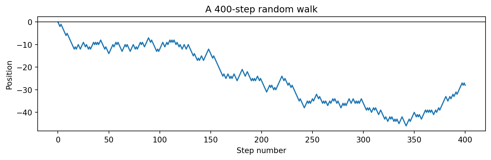
```{python}
import random
import numpy as np
import matplotlib.pyplot as plt

random.seed(42)
N = 400
steps = [random.choice([-1, 1]) for _ in range(N)]
# np.cumsum(steps)[k] = position after step k+1
positions = np.cumsum(steps)
# Prepend 0 so the plot starts at the origin
all_pos = [0] + list(positions)

fig, ax = plt.subplots(figsize=(9, 3))
ax.plot(range(0, N + 1), all_pos)
ax.axhline(0, color='black', linewidth=0.8)
ax.set_xlabel("Step number")
ax.set_ylabel("Position")
ax.set_title("A 400-step random walk")
plt.tight_layout()
plt.show()
```
The path wanders with no fixed destination.
Every new seed of `random.seed` produces a completely
different curve.
Lay five walks side by side and the variety is overwhelming —
yet all five obey the same law, which we investigate next.
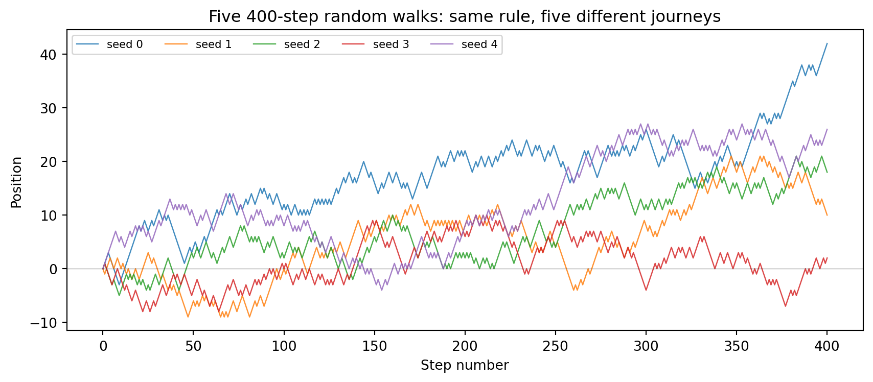
### Research Example: Does Every Walk Explore the Same Scale? {.unnumbered .unlisted}
Five walkers, five seeds, the same coin-flip rule — yet five completely
different journeys. Overlay them on one plot and ask: how far apart do
they wander, and is there any pattern in the spread?
```{python}
#| label: fig-walks-multi
#| fig-cap: "Five independent 400-step random walks with seeds 0–4. Same rule, five utterly different journeys."
import numpy as np
import matplotlib.pyplot as plt

COLORS = ['#1f77b4', '#ff7f0e', '#2ca02c', '#d62728', '#9467bd']

fig, ax = plt.subplots(figsize=(9, 4))
for i in range(5):
    rng_m = np.random.default_rng(i)
    steps_m = rng_m.choice([-1, 1], size=400)
    pos_m = np.concatenate([[0], np.cumsum(steps_m)])
    ax.plot(pos_m, lw=0.9, alpha=0.85, color=COLORS[i], label=f'seed {i}')
ax.axhline(0, color='black', lw=0.5, alpha=0.4)
ax.set_xlabel('Step number')
ax.set_ylabel('Position')
ax.set_title('Five 400-step random walks: same rule, five different journeys')
ax.legend(fontsize=8, ncol=5)
fig.tight_layout()
plt.show()
```
Every path looks different in detail, yet all five stay within the same
rough band — roughly $\pm\sqrt{400} = 20$ units from zero.
Boundless variety in the shape, iron regularity in the scale: that
is exactly what the square-root law, explored in the next section, captures.
---
## The Square-Root Rule {#sec-walks-sqrt}
A single walk gives no information about where walks
"typically" end up, because each one is unique.
To find a pattern we must average over many walks.
The **average final position** is zero by symmetry: left
and right steps cancel over many repetitions.
A better measure of "how far did the walk go?" is the
**root-mean-square (RMS) displacement**: square every
final position, average the squares, then take the
square root.
Squaring removes the sign, so a walk ending at $-20$ and
one ending at $+20$ contribute equally.
An elegant algebraic argument (no calculus needed) shows
that the RMS displacement after $N$ steps is exactly
$\sqrt{N}$.
Write the final position as
$X = s_1 + s_2 + \cdots + s_N$
where each step $s_k \in \{-1, +1\}$.
Expand the square:
$$X^2 = s_1^2 + s_2^2 + \cdots + s_N^2
+ \sum_{j \ne k} s_j\, s_k.$$
Each $s_k^2 = 1$ since $(\pm 1)^2 = 1$.
The cross terms $s_j s_k$ for $j \ne k$ average to zero
over many walks: because steps are independent and equally
likely $+1$ or $-1$, positive cross terms cancel negative
ones exactly.
So the average of $X^2$ is simply $N$, and therefore
$$\text{RMS displacement} = \sqrt{N}.$$
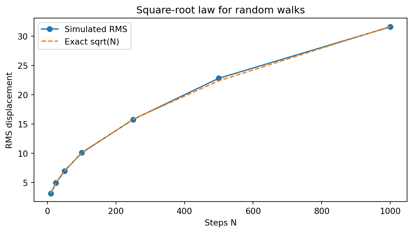
The code below checks this across two decades of step
counts.
```{python}
import random
import math

random.seed(0)
TRIALS = 2000
ns = [10, 25, 50, 100, 250, 500, 1000]
rms_vals = []
print(f"{'N':>5}  {'RMS':>7}  {'sqrt(N)':>8}")
print("-" * 24)
for N in ns:
    sum_sq = 0
    for _ in range(TRIALS):
        steps = [random.choice([-1, 1])
                 for _ in range(N)]
        pos = sum(steps)
        sum_sq += pos * pos
    rms = (sum_sq / TRIALS) ** 0.5
    rms_vals.append(rms)
    theory = math.sqrt(N)
    print(
        f"{N:>5}  {rms:>7.2f}  {theory:>8.3f}"
    )
```
Simulation and theory agree to within a fraction of a
percent.
A plot makes the square-root growth unmistakable.
```{python}
import matplotlib.pyplot as plt

theory_vals = [math.sqrt(N) for N in ns]

fig, ax = plt.subplots(figsize=(7, 4))
ax.plot(ns, rms_vals, 'o-',
        label='Simulated RMS')
ax.plot(ns, theory_vals, '--',
        label='Exact sqrt(N)')
ax.set_xlabel("Steps N")
ax.set_ylabel("RMS displacement")
ax.set_title("Square-root law for random walks")
ax.legend()
plt.tight_layout()
plt.show()
```
The square-root law has a practical interpretation: to
double the typical spread of a random process you must
quadruple the number of steps.
This is why diffusion is slow -- a molecule spreading
randomly through a liquid travels only $\sqrt{t}$ in
time $t$, not proportionally to $t$.
---
::: {.content-visible when-format="pdf"}
```{=latex}
\begin{center}
\begin{minipage}[c]{0.28\textwidth}
\centering
\href{https://youtu.be/iH2kATv49rc}{\includegraphics[width=\textwidth]{images/thumb_iH2kATv49rc.jpg}}
\end{minipage}%
\hspace{0.02\textwidth}%
\begin{minipage}[c]{0.28\textwidth}
\small\textbf{Mathemaniac}\\[3pt]
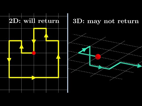
\small Random walks in 2D and 3D are fundamentally different\\[3pt]
\small\href{https://youtu.be/iH2kATv49rc}{\texttt{youtu.be/iH2kATv49rc}}
\end{minipage}%
\hspace{0.02\textwidth}%
\begin{minipage}[c]{0.36\textwidth}
\small A drunk man always finds his way home in 2D, but a drunk bird in 3D may wander lost forever --- why return probability drops from 1 to about 34\% when you add a third dimension.
\end{minipage}
\end{center}
```
:::
::: {.content-visible when-format="html"}
<div style="display:flex; align-items:flex-start; margin:1em 0; gap:12px; width:100%;">
<div style="flex:0 0 200px;"><a href="https://youtu.be/iH2kATv49rc" target="_blank"><img src="https://img.youtube.com/vi/iH2kATv49rc/0.jpg" style="width:100%;display:block;" alt="Random walks in 2D and 3D are fundamentally different"></a></div>
<div style="flex:1; font-size:0.85em;"><strong>Mathemaniac</strong><br>Random walks in 2D and 3D are fundamentally different<br><a href="https://youtu.be/iH2kATv49rc" target="_blank" style="font-family:monospace;">youtu.be/iH2kATv49rc</a></div>
<div style="flex:1; font-size:0.85em;">A drunk man always finds his way home in 2D, but a drunk bird in 3D may wander lost forever — why return probability drops from 1 to about 34% when you add a third dimension.</div>
</div>
:::
## 2D Random Walks {#sec-walks-2d}
```{python}
#| echo: false
from pathlib import Path; import urllib.request
_d = Path('images'); _d.mkdir(exist_ok=True)
_p = _d / 'polya.jpg'
if not _p.exists():
try: urllib.request.urlretrieve('https://upload.wikimedia.org/wikipedia/commons/5/5a/George_P%C3%B3lya_ca_1973.jpg', _p)
except Exception: pass
```
::: {.content-visible when-format="pdf"}
```{=latex}
\begin{center}
\begin{minipage}[c]{0.22\textwidth}
\includegraphics[width=\textwidth]{images/polya.jpg}
\end{minipage}%
\hspace{0.03\textwidth}%
\begin{minipage}[c]{0.55\textwidth}
\small\textit{George Pólya (1887--1985)}\\[2pt]
\tiny CC BY 2.0, Thane Plambeck, via Wikimedia Commons
\end{minipage}
\end{center}
```
:::
::: {.content-visible when-format="html"}
<div style="display:flex; align-items:center; margin:1em 0; gap:12px;">
<img src="images/polya.jpg" style="width:100px; flex-shrink:0;" alt="George Pólya">
<div style="font-size:0.82em;"><em>George Pólya (1887–1985)</em><br><span style="font-size:0.85em;">CC BY 2.0, Thane Plambeck, via Wikimedia Commons</span></div>
</div>
:::
A random walk need not be confined to a line.
Place a walker on an infinite square grid and at each
step let them move one unit North, South, East, or West
with equal probability $\frac{1}{4}$.
This is a **two-dimensional random walk**.
The square-root law still holds: typical distance from
the origin is approximately $\sqrt{N}$ after $N$ steps.
But a new phenomenon emerges.
In 1921 George Polya proved that a 2D random walk is
**recurrent**: no matter how far the walker may wander,
the probability of eventually returning to the starting
square is exactly 1 [@polya1921].
The same is true in one dimension.
In three dimensions (six directions: $\pm x$, $\pm y$,
$\pm z$), however, the walk is **transient**: the
probability of ever returning to the origin is only about
$34\%$.
Research topic 9 asks you to verify this computationally.
```{python}
import random
import matplotlib.pyplot as plt

random.seed(7)
DIRS = [(1, 0), (-1, 0), (0, 1), (0, -1)]
N = 500
x, y = 0, 0
xs, ys = [0], [0]
for _ in range(N):
    dx, dy = random.choice(DIRS)
    x += dx
    y += dy
    xs.append(x)
    ys.append(y)

fig, ax = plt.subplots(figsize=(6, 6))
ax.plot(xs, ys, linewidth=0.5, alpha=0.7)
ax.plot(0, 0, 'go', markersize=8,
        label='Start')
ax.plot(xs[-1], ys[-1], 'r*',
        markersize=12, label='End')
ax.set_aspect('equal')
ax.legend()
ax.set_title("500-step 2D random walk")
plt.tight_layout()
plt.show()
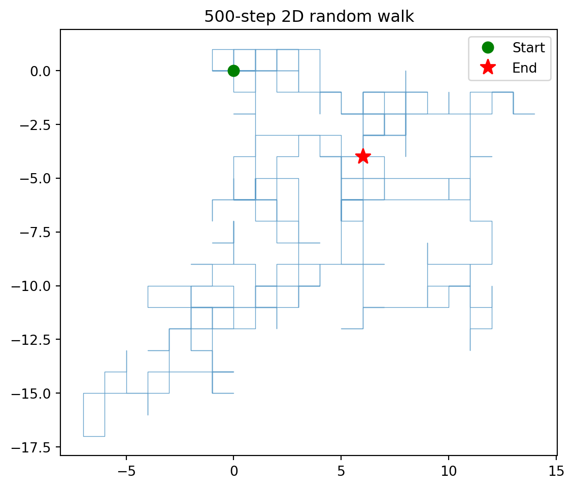
```
The walk fills a roughly circular region centered on the
origin, with ragged arms extending in all directions.
The start (green circle) and the end (red star) are
typically far apart -- the walk rarely ends where it
began, even though it is guaranteed to return eventually.
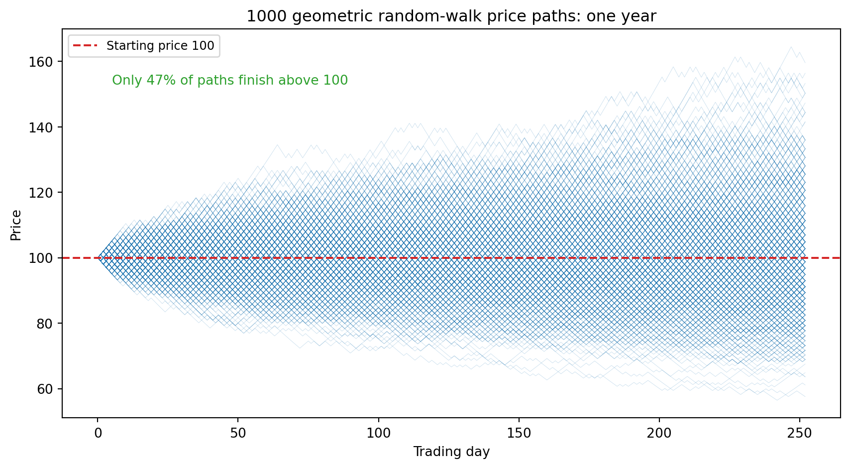
The same mathematics governs stock prices.
Each trading day a price multiplies by a random factor —
up 1% or down 1% with equal probability.
That sounds symmetric, but the multiplicative structure
hides a trap: $\log(1.01) + \log(0.99) < 0$,
so the geometric mean of each step is slightly below 1.
Run 1,000 price paths for a full trading year
and watch where they finish.
### Research Example: Does a Fair Coin Flip Ruin a Stock? {.unnumbered .unlisted}
A stock that goes up 1% or down 1% with equal probability sounds like a fair game —
wins and losses are identical in size. Does running 1,000 such price paths for a full
year (252 trading days) confirm that intuition, or reveal a hidden drift?
```{python}
#| label: fig-walks-stock
#| fig-cap: "1,000 geometric random-walk stock price paths over 252 trading days. Multiplying by 1.01 or 0.99 each day with equal probability looks symmetric but drifts most paths below the starting price."
import numpy as np
import matplotlib.pyplot as plt

BLUE = '#1f77b4'
RED  = '#d62728'
GREEN = '#2ca02c'

rng_s = np.random.default_rng(42)
DAYS = 252
PATHS = 1000
factors = rng_s.choice([1.01, 0.99], size=(PATHS, DAYS))
prices = np.hstack([np.full((PATHS, 1), 100.0),
                    100.0 * np.cumprod(factors, axis=1)])

fig, ax = plt.subplots(figsize=(9, 5))
for p in prices:
    ax.plot(p, lw=0.25, alpha=0.3, color=BLUE)
ax.axhline(100, color=RED, lw=1.5, ls='--', label='Starting price 100')
pct_above = 100 * np.mean(prices[:, -1] > 100)
ax.text(5, prices.max() * 0.93,
        f'Only {pct_above:.0f}% of paths finish above 100',
        color=GREEN, fontsize=10)
ax.set_xlabel('Trading day')
ax.set_ylabel('Price')
ax.set_title(f'{PATHS} geometric random-walk price paths: one year')
ax.legend(fontsize=9)
fig.tight_layout()
plt.show()
```
The coin flip is mathematically fair, yet fewer than half the paths end above the
starting price — the multiplicative structure punishes losses more than gains reward.
A 1% gain followed by a 1% loss leaves you at 99.99, not 100: the walk drifts downward
even when the coin is perfectly balanced.
---
## First Return Times {#sec-walks-return}
How long does a 1D walk take to first come back to
position zero?
Two facts are immediately clear.
The return time is always even: the walk must accumulate
equal counts of $+1$ and $-1$ steps to reach zero, and
that sum is always even.
And in 1D the return always happens -- the recurrence
guarantee means no walk can escape forever.
The minimum return time is 2, and it happens more often
than you might expect.
The walk must take one step away (say $+1$) and then one
step back ($-1$), or vice versa.
Each such two-step sequence has probability
$\frac{1}{2} \times \frac{1}{2} = \frac{1}{4}$, and
there are two such sequences, so
$$P(\text{first return at step } 2) = \frac{1}{2}.$$
Half of all random walks come home in just two steps!
The other half may take much, much longer.
In fact the **mean** return time is infinite: occasional
walks that wander far pull the average up without bound.
The median is a better summary, and we confirm it by
simulation.
```{python}
import random

def first_return_1d(max_steps=10_000):
    pos = 0
    for t in range(1, max_steps + 1):
        pos += random.choice([-1, 1])
        if pos == 0:
            return t
    return None  # did not return within cap

random.seed(1)
TRIALS = 3000
returns = []
for _ in range(TRIALS):
    t = first_return_1d()
    if t is not None:
        returns.append(t)

never = TRIALS - len(returns)
pct = 100 * len(returns) / TRIALS
print(f"Returned:      {len(returns)}/{TRIALS}")
print(f"Not returned:  {never}")
print(f"Fraction back: {pct:.2f}%")
```
Almost every walk returns within the 10,000-step cap,
confirming recurrence.
```{python}
s_r = sorted(returns)
med = s_r[len(s_r) // 2]
mean_r = sum(returns) / len(returns)
print(f"Shortest return: {s_r[0]}")
print(f"Median return:   {med}")
print(f"Mean return:     {mean_r:.0f}")
print(f"Longest return:  {s_r[-1]}")
print()
print(f"{'t':>5}  {'count':>6}  {'frac':>6}")
print("-" * 22)
for t in range(2, 22, 2):
    cnt = returns.count(t)
    print(
        f"{t:>5}  {cnt:>6}  "
        f"{cnt/TRIALS:>6.3f}"
    )
```
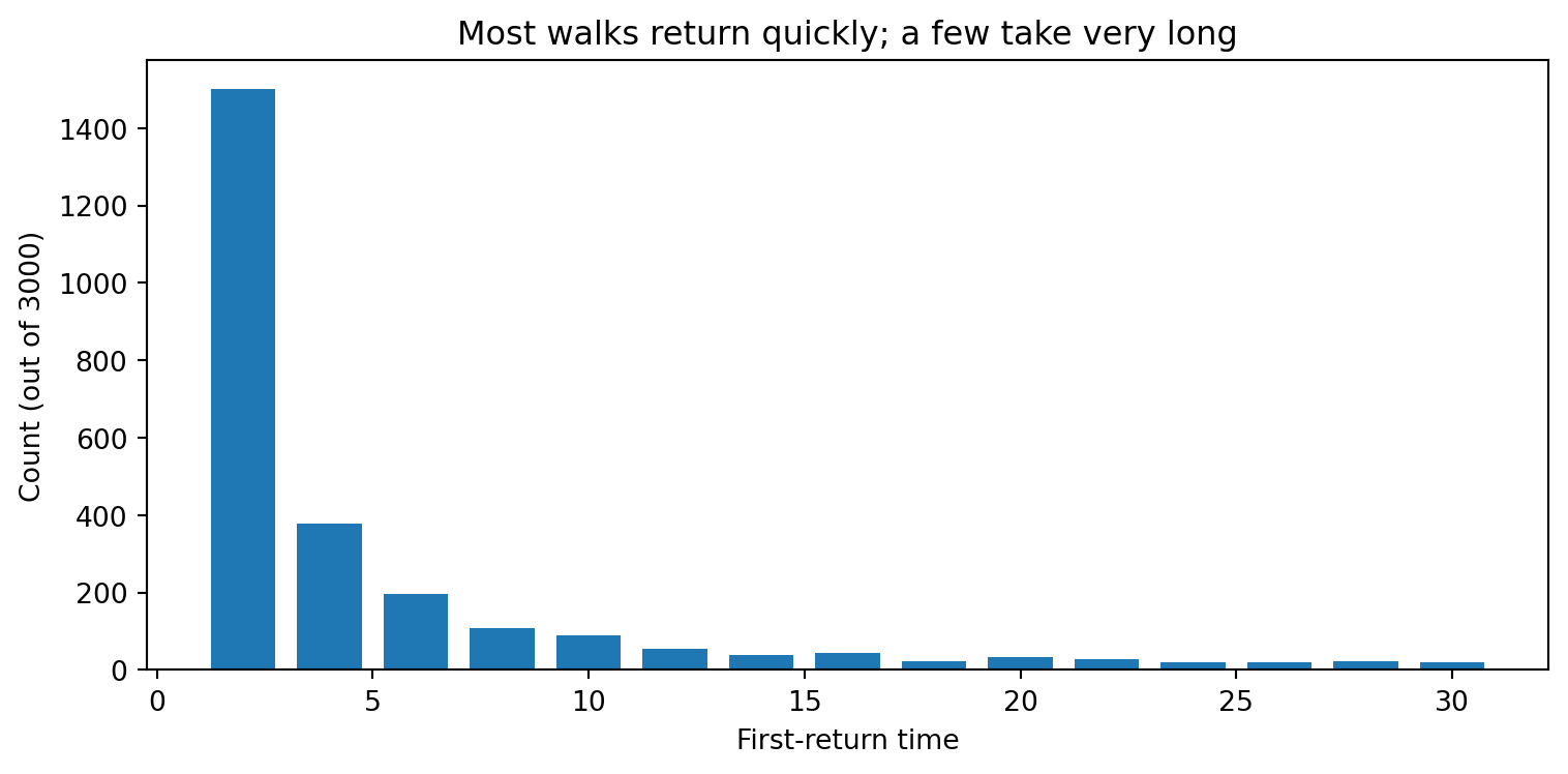
The median is 2: more than half of all walks return in
just two steps.
The mean is far larger because a small fraction of walks
take hundreds or thousands of steps to return, dragging
the average upward.
The count table shows this asymmetry: the first row alone
accounts for about 50% of all returns, the next few rows
share the next 30%, and the remaining 20% is spread across
all longer return times.
```{python}
import matplotlib.pyplot as plt

# Bar chart for first-return times 2 through 30
ts = list(range(2, 32, 2))
cnts = [returns.count(t) for t in ts]

fig, ax = plt.subplots(figsize=(8, 4))
ax.bar(ts, cnts, width=1.5)
ax.set_xlabel("First-return time")
ax.set_ylabel("Count (out of 3000)")
ax.set_title(
    "Most walks return quickly; "
    "a few take very long"
)
plt.tight_layout()
plt.show()
```
The tall bar at $t = 2$ dominates.
The remaining bars form a long, heavy tail -- the
signature of a **power-law distribution**, where the
probability of a very long return shrinks slowly rather
than exponentially.
---
## Diffusion and the Normal Distribution {#sec-walks-diffusion}
Run 10,000 independent 1D walks of $N = 100$ steps.
Record only the final position of each walk.
The 10,000 numbers range roughly from $-40$ to $+40$.
Is there any pattern to where they land?
```{python}
import random
import math
import matplotlib.pyplot as plt

random.seed(3)
TRIALS = 10_000
N = 100
finals = []
for _ in range(TRIALS):
    steps = [random.choice([-1, 1])
             for _ in range(N)]
    finals.append(sum(steps))

fig, ax = plt.subplots(figsize=(9, 4))
# ax.hist(data, bins, density=True) draws a
# histogram with total area = 1 so the curve
# below can overlay it directly.
ax.hist(
    finals,
    bins=range(-50, 52, 2),
    density=True,
    alpha=0.6,
    label='Simulation'
)

# Overlay the normal (bell) curve with mean 0
# and standard deviation sqrt(N) = 10.
sigma = math.sqrt(N)
xs_c = [x / 5 for x in range(-250, 251)]
gauss = []
for x in xs_c:
    e_val = math.exp(-x * x / (2 * N))
    denom = sigma * math.sqrt(2 * math.pi)
    gauss.append(e_val / denom)
ax.plot(
    xs_c, gauss, 'r-', linewidth=2,
    label=f'Normal (mean=0, sd={sigma:.0f})'
)
ax.set_xlabel("Final position")
ax.set_ylabel("Probability density")
ax.legend()
ax.set_title(
    f"{TRIALS} walks of N={N} steps each", loc='center'
)
plt.tight_layout()
plt.show()
```
The histogram fits the red curve almost perfectly.
That red curve is the **normal distribution** (also
called the Gaussian or bell curve).
Why does a normal distribution appear here?
Each step is a tiny random push of $+1$ or $-1$.
The final position is the sum of 100 such pushes.
The **Central Limit Theorem** states that the sum of
many independent random quantities -- regardless of
their individual distribution -- converges to a normal
distribution as the number of terms grows [@demoivre1733; @laplace1812].
Our walk is precisely a sum of 100 independent $\pm 1$
variables, so the theorem applies.
The connection to physics is direct.
When a drop of ink falls into still water, each ink
molecule follows its own random walk as neighboring
water molecules push it left and right and up and down.
The spreading cloud of ink is the physical realization
of the histogram above: a bell curve that widens by
$\sqrt{t}$ in time $t$.
This process is called **diffusion**, and the
square-root law from @sec-walks-sqrt is exactly the
diffusion equation's prediction for the width of the
spreading cloud.
---
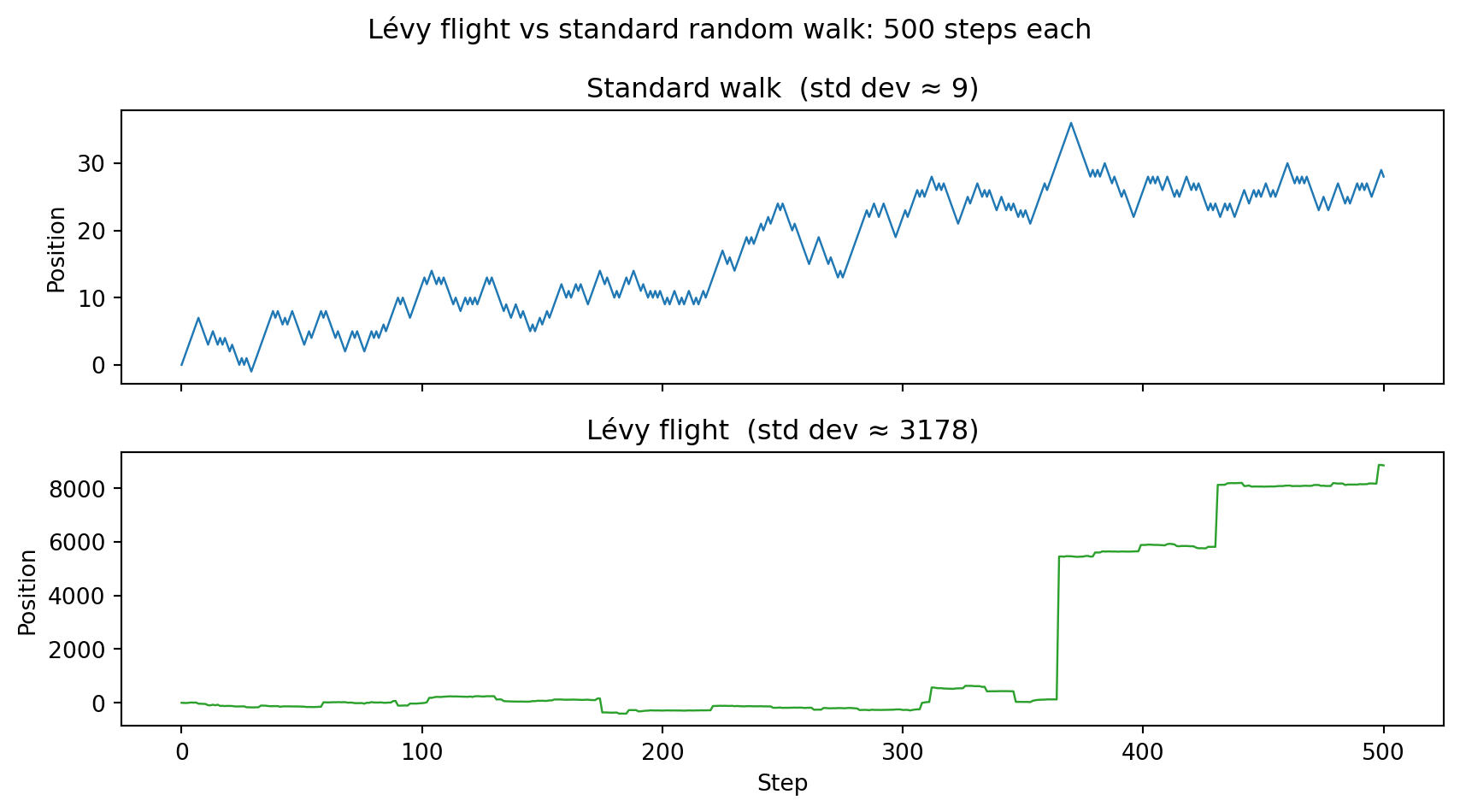
Not all random processes spread this slowly.
A **Lévy flight** draws each step size from a heavy-tailed
distribution: rare, enormous jumps appear that dwarf
anything seen in a standard walk.
Animal foraging paths, light in turbulent media, and
some financial price moves all show Lévy-flight statistics —
wild leaps that the square-root law cannot capture.
### Research Example: How Different Is a Walk With Giant Leaps? {.unnumbered .unlisted}
A standard walk takes steps of exactly $\pm 1$, but what if step sizes follow a
heavy-tailed law where huge jumps are rare but possible? Pit a Lévy flight against
a standard walk over the same 500 steps and see whether the difference is visible.
```{python}
#| label: fig-walks-levy
#| fig-cap: "Lévy flight vs standard random walk, both 500 steps. The Lévy flight makes rare giant leaps; the standard walk stays close to its starting point by comparison."
import numpy as np
import matplotlib.pyplot as plt

BLUE  = '#1f77b4'
GREEN = '#2ca02c'

rng_l = np.random.default_rng(7)
N_l = 500
std_steps_l = rng_l.choice([-1, 1], size=N_l).astype(float)
std_pos_l = np.concatenate([[0], np.cumsum(std_steps_l)])

u = rng_l.uniform(0, 1, size=N_l)
levy_sizes = np.ceil(1 / u**1.5)
levy_dirs = rng_l.choice([-1, 1], size=N_l)
levy_pos = np.concatenate([[0], np.cumsum(levy_sizes * levy_dirs)])

fig, axes = plt.subplots(2, 1, figsize=(9, 5), sharex=True)
axes[0].plot(std_pos_l, lw=0.9, color=BLUE)
axes[0].set_ylabel('Position')
axes[0].set_title(f'Standard walk  (std dev ≈ {np.std(std_pos_l):.0f})')
axes[1].plot(levy_pos, lw=0.9, color=GREEN)
axes[1].set_ylabel('Position')
axes[1].set_xlabel('Step')
axes[1].set_title(f'Lévy flight  (std dev ≈ {np.std(levy_pos):.0f})')
fig.suptitle('Lévy flight vs standard random walk: 500 steps each')
fig.tight_layout()
plt.show()
```
The standard walk inches along in a narrow band, while the Lévy flight rockets to
positions hundreds or thousands of times further with just a single lucky step.
The square-root law breaks down completely: rare events dominate, and the spread
grows far faster than $\sqrt{N}$.
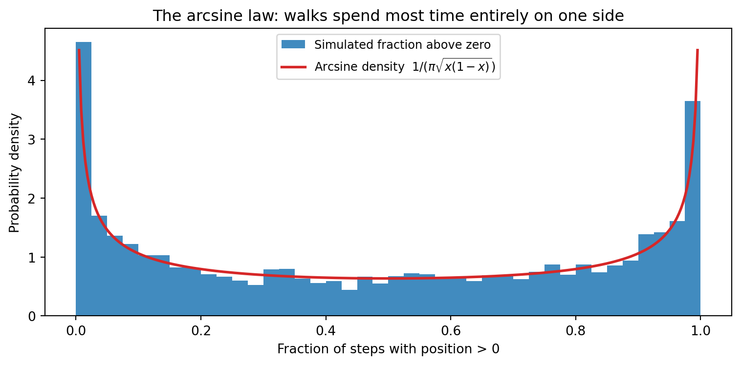
Perhaps the most counterintuitive fact about random walks is the
**arcsine law**: for 1D walks, the fraction of time spent above zero
does not peak near one-half.
Instead it piles up near 0 and 1.
A walker who is ahead at the halfway point is more likely to lead
the entire second half than to fall behind.
Run 5,000 walks and the picture is unmistakable.
### Research Example: Does a Fair Walk Split Its Time Fairly Above Zero? {.unnumbered .unlisted}
Intuition says a fair random walk should spend roughly half its time above zero and
half below. Does simulation back that up, or does the histogram of "fraction of time
above zero" tell a more surprising story?
```{python}
#| label: fig-walks-arcsine
#| fig-cap: "Arcsine law: fraction of time each of 5,000 walks (1,000 steps each) spends above zero. The mass piles up at both ends — walks tend to stay above or below zero for the bulk of their journey, not oscillate around it."
import numpy as np
import math
import matplotlib.pyplot as plt

BLUE = '#1f77b4'
RED  = '#d62728'

rng_a = np.random.default_rng(99)
WALKS_A = 5000
STEPS_A = 1000
steps_all = rng_a.choice([-1, 1], size=(WALKS_A, STEPS_A))
positions_a = np.cumsum(steps_all, axis=1)
frac_pos = np.mean(positions_a > 0, axis=1)

xs_arc = np.linspace(0.005, 0.995, 300)
arcsine_pdf = 1.0 / (math.pi * np.sqrt(xs_arc * (1 - xs_arc)))

fig, ax = plt.subplots(figsize=(8, 4))
ax.hist(frac_pos, bins=40, density=True, color=BLUE, alpha=0.85,
        label='Simulated fraction above zero')
ax.plot(xs_arc, arcsine_pdf, color=RED, lw=2,
        label='Arcsine density  $1/(\pi\sqrt{x(1-x)})$')
ax.set_xlabel('Fraction of steps with position > 0')
ax.set_ylabel('Probability density')
ax.set_title('The arcsine law: walks spend most time entirely on one side')
ax.legend(fontsize=9)
fig.tight_layout()
plt.show()
```
The histogram is shaped like a U, not a bell — most walks spend nearly all their time
on one side of zero, not oscillating evenly. The red arcsine curve $1/(\pi\sqrt{x(1-x)})$
fits the data precisely, confirming that "staying on one side" is the rule, not the exception.
---
## Further Research Topics {#sec-walks-research}
2. **A biased walk.**
Modify the 1D walk so that each step is $+1$ with
probability $p = 0.6$ and $-1$ with probability
$p = 0.4$.
The function `random.choices([-1, 1],
weights=[0.4, 0.6])[0]` draws a single biased step.
Run 1000 walks of 500 steps each and plot the
distribution of final positions.
How does the average final position compare to the
unbiased case?
How does the standard deviation compare?
*(Problem proposed by Claude Code.)*
3. **The Gambler's Ruin.**
A gambler starts with \$10 and bets \$1 on a fair coin
flip each round.
The game ends when they reach \$0 (ruined) or \$20
(they doubled their money).
Theory predicts exactly 50% ruin probability for a
fair game.
Simulate 10,000 games and verify.
Then repeat with a slightly biased coin (probability
0.51 of winning each flip) and measure how the ruin
probability changes with only a tiny bias.
*(Problem proposed by Claude Code.)*
4. **Counting returns to zero.**
For a 1D walk of $N$ steps, count the total number
of times the walk visits position zero (not just the
first return).
Average this count over 2000 walks.
Compute this for $N = 100, 400, 900, 1600, 2500$.
How does the expected number of returns to zero grow
with $N$?
Plot the data and look for a power-law pattern.
(Theory predicts growth proportional to $\sqrt{N}$.)
*(Problem proposed by Claude Code.)*
5. **First passage to a wall.**
Starting at position 0, measure the first time the
walk reaches position $+20$.
Simulate 2000 walks (cap each at 200,000 steps).
Plot the histogram of first-passage times.
What is the median?
Does the mean appear to converge or grow without
bound as more walks are simulated?
Compare the shape of this distribution to the
first-return distribution from @sec-walks-return.
*(Problem proposed by Claude Code.)*
6. **2D return time.**
Adapt the 2D walk code to find the first step at
which the walker returns to $(0, 0)$.
Simulate 2000 two-dimensional walks capped at
100,000 steps each.
What fraction return within the cap?
Compare the median return time to the 1D case.
In 2D the walk is still recurrent, but returns are
far rarer -- how much rarer?
*(Problem proposed by Claude Code.)*
7. **Cover time on a finite grid.**
Walk on an $n \times n$ grid with wraparound:
stepping off one edge reappears at the opposite edge
(a torus).
The **cover time** is the first step when every one
of the $n^2$ cells has been visited at least once.
Simulate 200 walks for $n = 5, 10, 15, 20$ and
record the average cover time.
Plot average cover time against $n^2$ (the number
of cells) and determine the approximate relationship.
*(Problem proposed by Claude Code.)*
9. **3D transience.**
In three dimensions the walk moves in six directions:
$(\pm 1, 0, 0)$, $(0, \pm 1, 0)$, $(0, 0, \pm 1)$,
each with probability $\frac{1}{6}$.
Polya proved that such a walk is transient: it returns
to the origin with probability only about 0.34 [@polya1921].
Simulate 2000 three-dimensional walks of 50,000 steps
each and measure the fraction that visit $(0, 0, 0)$
at least once after the start.
Compare this to the 2D case you explored in
@sec-walks-2d.
*(Problem proposed by Claude Code.)*
11. **Self-avoiding walks.**
A self-avoiding walk cannot revisit any grid square.
Using backtracking (try each direction; if it leads
to a previously visited cell, back up and try the
next direction), enumerate all self-avoiding walks
of length 1 through 10 starting at $(0, 0)$ on a
2D grid.
Count the walks for each length.
The counts grow approximately as $\mu^n$ for some
constant $\mu$ -- estimate $\mu$ from your data [@orr1947].
*(Problem proposed by Claude Code.)*
12. **The Polya urn** [@polya1923]**.**
Start with 1 red ball and 1 blue ball in an urn.
At each step, draw one ball at random, return it,
and add one new ball of the same color.
After 10,000 draws, record the fraction of red balls.
Repeat 10,000 times and plot the distribution of
final fractions.
Every fraction between 0 and 1 is equally likely --
the distribution is uniform!
Verify this computationally and compute the mean and
standard deviation of the fraction.
*(Problem proposed by Claude Code.)*
13. **Random walk temperature solver.**
Set up a $21 \times 21$ grid.
Fix all boundary cells (the edges) to temperature 0.
Fix the single center cell at position $(10, 10)$
to temperature 100.
To estimate the temperature at any interior cell
$(r, c)$, launch many random walks from $(r, c)$;
each walk continues until it hits either the boundary
or the center.
Average the temperatures at the stopping cells.
Implement this for the five cells nearest the center
and compare to the expected decay.
This Monte Carlo approach is related to how computers
solve the Laplace equation for heat or electricity [@kakutani1944].
*(Problem proposed by Claude Code.)*
14. **Loop-erased random walk.**
A loop-erased random walk removes loops from a
standard walk: whenever the path revisits a site,
erase the entire loop from the first visit to the
re-visit.
Generate 100 loop-erased walks of 300 steps on a
2D grid and record how many steps survive after
erasure.
The loop-erased walk is conjectured to have fractal
dimension $\frac{5}{4}$ in 2D [@lawler1980].
Estimate this dimension using the box-counting
method from @sec-fractals-dimension.
*(Problem proposed by Claude Code.)*
15. **Random walks and electrical networks.**
In a resistor network, the probability that a random
walk from node $A$ reaches node $B$ before node $C$
equals the voltage at $A$ when $B$ is held at 1 volt
and $C$ at 0 volts [@kakutani1944].
Build a chain of 7 nodes (numbered 0 through 6),
with node 0 held at voltage 1 and node 6 at voltage
0.
From each interior node $k$ (1 through 5), simulate
1000 random walks and record the fraction that reach
node 0 before node 6.
The true voltage at node $k$ is $1 - k/6$.
How well does your simulation match the formula?
*(Problem proposed by Claude Code.)*
17. **PageRank as a stationary random walk.**
Build a directed graph of 6 web pages: A links to B
and C; B links to C; C links to A and D; D links to
A, B, and E; E links to F; F links back to A.
Set up the transition matrix $P$ as a $6 \times 6$
NumPy array where $P[i][j]$ is the probability of
jumping from page $i$ to page $j$ (uniform over all
outgoing links from $i$) [@brin1998].
The **PageRank** of each page is the long-run fraction
of time a random surfer spends there.
Compute it two ways and compare:
(a) Simulate 1,000,000 steps of the random walk and
record visit fractions.
(b) Multiply $P$ by itself 1000 times using
`numpy.linalg.matrix_power(P, 1000)` -- any row of
this matrix is the stationary distribution (no
eigenvectors needed; repeated multiplication is enough).
How do the rankings change if you add a new link from
F to D?
Which page has the highest rank and why?
*(Problem proposed by Claude Code.)*
18. **The ballot problem and the reflection principle.**
Candidate A receives 7 votes and candidate B receives
3 votes.
In how many of the $\binom{10}{3} = 120$ orderings
of the ballots does A lead B strictly throughout the
entire count?
The **ballot theorem** [@bertrand1887] predicts exactly
$(7 - 3)/(7 + 3) = 40\%$ of orderings.
Verify by brute force: use `itertools.combinations`
to generate every way to place 3 B-votes among 10
ballot positions, simulate the running tally for each,
and count those where A is strictly ahead at every step.
Then test the formula $(a - b)/(a + b)$ for at least
five other $(a, b)$ pairs with $a > b$.
Finally, draw the walk as a lattice path (A-vote = step
up, B-vote = step down) and sketch the **reflection
principle**: every "bad" path that touches or crosses
zero corresponds to exactly one reflected path starting
from $-1$.
Can you turn this geometric picture into a proof of
the formula?
*(Problem proposed by Claude Code.)*
19. **Brownian motion as the limit of rescaled walks** [@wiener1923]**.**
Fix a time window of length 1.
For $n = 10, 100, 1000$, simulate a random walk of
$n$ steps where each step has size $\pm 1/\sqrt{n}$,
so the walk always spans the same "time" $[0, 1]$
regardless of $n$.
Plot 5 sample paths for each $n$ on separate axes.
As $n$ grows the jagged zigzag smooths out into a
curve that looks almost continuous -- yet its
statistics stay the same: the standard deviation of
the position at time $t = 0.5$ is always $\sqrt{0.5}$
regardless of $n$.
Verify this experimentally by running 2000 walks for
each $n$ and measuring the standard deviation at the
halfway point.
Then apply the box-counting method from
@sec-fractals-dimension to a single long path
($n = 10{,}000$) and estimate its fractal dimension.
Theory predicts a value of $\frac{3}{2}$
(for the graph of the path as a curve in the plane) --
how close does your simulation get?
*(Problem proposed by Claude Code.)*
20. **Wilson's algorithm: spanning trees from loop-erased walks.**
A **spanning tree** of a graph is a subset of edges
that connects every vertex with no cycles.
**Wilson's algorithm** (1996) generates a uniformly
random spanning tree using the loop-erased walk
from topic 14 as its building block: start from an
unvisited vertex, walk randomly until reaching an
already-included vertex, erase any loops, add the
resulting path to the tree; repeat until all vertices
are included [@wilson1996].
Implement Wilson's algorithm on a $5 \times 5$ grid
(25 vertices), making sure the loop-erasure step
follows the same logic as in topic 14.
Generate 20 random spanning trees and draw each one
using matplotlib.
Record the degree (number of tree-edges attached) of
each vertex across your 20 trees.
Do corner vertices, edge vertices, and interior
vertices appear to have different average degrees?
As an extension, compare your uniformly random trees
to spanning trees produced by Kruskal's algorithm with
random edge weights: are the two distributions
identical or different, and how can you test this?
*(Problem proposed by Claude Code.)*