# The Logistic Map: Chaos from a Simple Equation {#sec-logistic}
## A Model for Population Growth {#sec-logistic-model}
Imagine a species of moths living in a forest.
If the forest is nearly empty this year, the moth population
will explode next year -- plenty of food, no crowding.
If the forest is packed to capacity, starvation and disease
will cut the population back sharply the following year.
Neither extreme lasts; the population bounces between them
in patterns that can range from steady to surprisingly wild.
```{python}
#| echo: false
from pathlib import Path; import urllib.request
_d = Path('images'); _d.mkdir(exist_ok=True)
_p = _d / 'pierre_verhulst.jpg'
if not _p.exists():
try: urllib.request.urlretrieve('https://upload.wikimedia.org/wikipedia/commons/0/04/Pierre_Francois_Verhulst.jpg', _p)
except Exception: pass
```
::: {.content-visible when-format="pdf"}
```{=latex}
\begin{center}
\begin{minipage}[c]{0.22\textwidth}
\includegraphics[width=\textwidth]{images/pierre_verhulst.jpg}
\end{minipage}%
\hspace{0.03\textwidth}%
\begin{minipage}[c]{0.55\textwidth}
\small\textit{Pierre Verhulst (1804--1849)}\\[2pt]
\tiny Public domain, via Wikimedia Commons
\end{minipage}
\end{center}
```
:::
::: {.content-visible when-format="html"}
<div style="display:flex; align-items:center; margin:1em 0; gap:12px;">
<img src="images/pierre_verhulst.jpg" style="width:100px; flex-shrink:0;" alt="Pierre Verhulst">
<div style="font-size:0.82em;"><em>Pierre Verhulst (1804–1849)</em><br><span style="font-size:0.85em;">Public domain, via Wikimedia Commons</span></div>
</div>
:::
In 1838, the Belgian mathematician Pierre Verhulst captured
both forces in one equation [@verhulst1838]. Let $x_n$ be the population
as a **fraction of the maximum the environment can support**,
so $0 \le x_n \le 1$. A value of $x_n = 0.2$ means the
habitat is at 20% capacity; $x_n = 0.9$ means it is nearly
full. The **logistic map** says:
$$x_{n+1} = r \cdot x_n \cdot (1 - x_n)$$
The parameter $r > 0$ is the **growth rate** -- how fast the
population would multiply if resources were unlimited.
The factor $(1 - x_n)$ is the **resource brake**: close to
1 when the habitat is empty, shrinking toward 0 as crowding
sets in.
This one equation, innocent enough for a high-school
algebra class, hides a universe of behavior.
```{python}
def logistic(r, x):
    return r * x * (1 - x)

r = 2.5
x = 0.1          # start at 10% of capacity

print(f"{'Step':>5}  {'Population':>12}")
print("-" * 22)
for step in range(1, 21):
    x = logistic(r, x)
    print(f"{step:>5}  {x:.8f}")
```
For $r = 2.5$ the population settles to a fixed fraction
and stays there. The **fixed point** satisfies
$x^* = r x^*(1 - x^*)$, which (dividing both sides by
$x^* \ne 0$) gives $x^* = 1 - 1/r$. For $r = 2.5$,
$x^* = 0.6$. The code confirms it: after a few
oscillations the sequence locks onto 0.6.
The fixed point exists for $r > 1$ (at $x^* = 1 - 1/r$)
together with the trivial fixed point $x^* = 0$. But
"exists" and "stable" are different things. Whether
the orbit *converges* to $x^*$ depends on $r$.
::: {.content-visible when-format="pdf"}
```{=latex}
\begin{center}
\begin{minipage}[c]{0.28\textwidth}
\centering
\href{https://youtu.be/ovJcsL7vyrk}{\includegraphics[width=\textwidth]{images/thumb_ovJcsL7vyrk.jpg}}
\end{minipage}%
\hspace{0.02\textwidth}%
\begin{minipage}[c]{0.28\textwidth}
\small\textbf{Veritasium}\\[3pt]
\small This Equation Will Change How You See the World\\[3pt]
\small\href{https://youtu.be/ovJcsL7vyrk}{\texttt{youtu.be/ovJcsL7vyrk}}
\end{minipage}%
\hspace{0.02\textwidth}%
\begin{minipage}[c]{0.36\textwidth}
\small One simple equation --- $x_{n+1} = rx_n(1-x_n)$ --- connects population biology, fluid turbulence, neuron firing, and the Mandelbrot set through the same bifurcation cascade.
\end{minipage}
\end{center}
```
:::
::: {.content-visible when-format="html"}
<div style="display:flex; align-items:flex-start; margin:1em 0; gap:12px; width:100%;">
<div style="flex:0 0 200px;"><a href="https://youtu.be/ovJcsL7vyrk" target="_blank"><img src="https://img.youtube.com/vi/ovJcsL7vyrk/0.jpg" style="width:100%;display:block;" alt="This Equation Will Change How You See the World"></a></div>
<div style="flex:1; font-size:0.85em;"><strong>Veritasium</strong><br>This Equation Will Change How You See the World<br><a href="https://youtu.be/ovJcsL7vyrk" target="_blank" style="font-family:monospace;">youtu.be/ovJcsL7vyrk</a></div>
<div style="flex:1; font-size:0.85em;">One simple equation — x_(n+1) = rx_n(1−x_n) — connects population biology, fluid turbulence, neuron firing, and the Mandelbrot set through the same bifurcation cascade.</div>
</div>
:::
## Iterating the Map {#sec-logistic-iterate}
The value of $r$ determines everything about long-run
behavior. Four qualitatively different regimes emerge as
$r$ grows from 1 to 4.
| Range of $r$ | Long-run behavior |
|-----------------------|-------------------------------------|
| $r < 1$ | Population dies out ($x_n \to 0$) |
| $1 < r < 3$ | Settles to one fixed point |
| $3 < r < 3.449\ldots$ | Alternates between two values |
| $3.449 < r < 3.544$ | Four-value cycle (then 8, then 16) |
| $r > 3.57$ (approx.) | Chaotic -- never repeats |
The boundary $r = 3$ is where the fixed point loses
stability. At that moment the orbit begins to alternate
between two values -- a **period-2 cycle** has bifurcated
from the fixed point. As $r$ grows further, the
period-2 cycle loses stability and splits into a period-4
cycle, then period-8, and so on in a **period-doubling
cascade**.
### Research Example: The Four Faces of the Logistic Map {.unnumbered .unlisted}
Can one equation produce a steady fixed point, a two-value oscillation, a four-cycle, and never-ending chaos — just by changing a single number?
We run 60 steps from $x_0 = 0.5$ at four growth rates to see all four regimes side by side.
```{python}
# uses: logistic()
#| label: fig-logistic-regimes
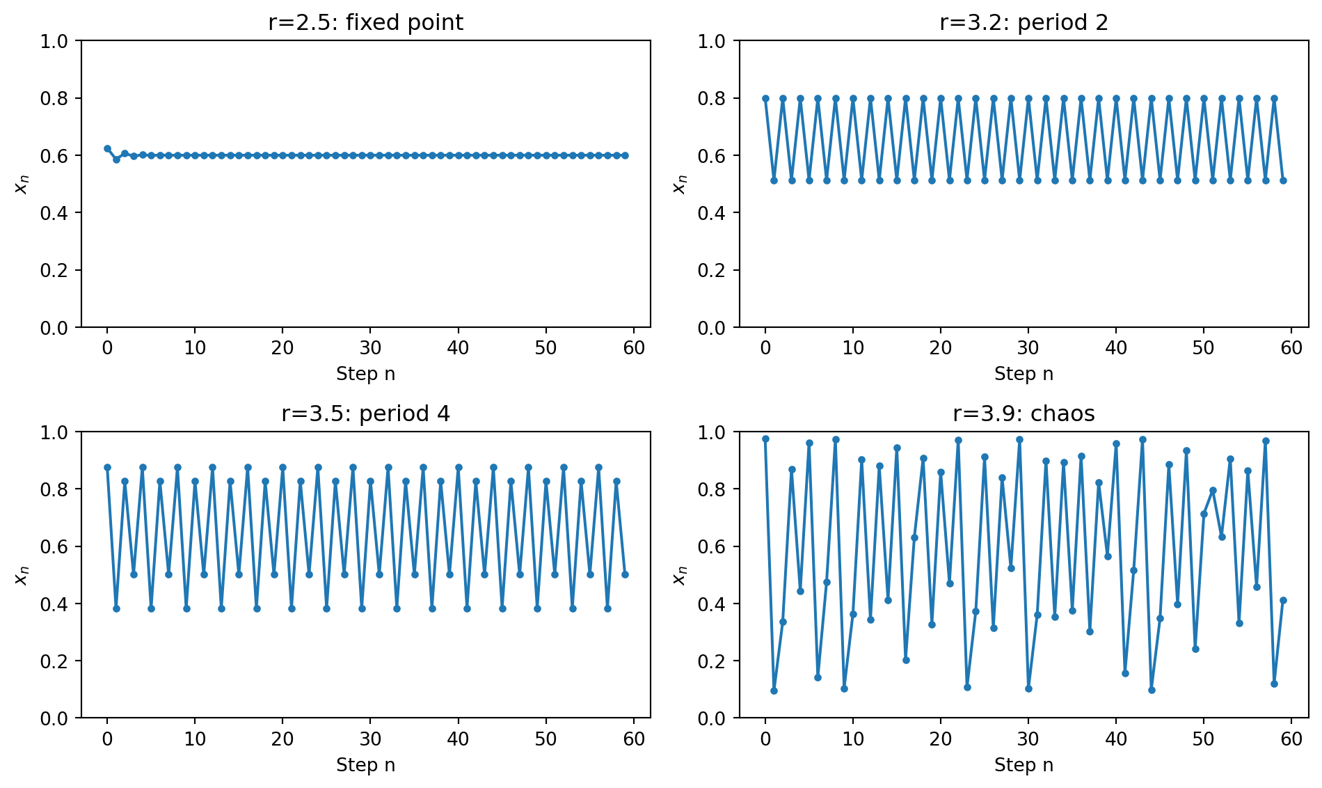
#| fig-cap: "Four regimes of the logistic map from a common start x0=0.5: fixed-point convergence (r=2.5), period-2 oscillation (r=3.2), period-4 cycle (r=3.5), and chaos (r=3.9). Each panel shows 60 steps of iteration."
import matplotlib.pyplot as plt
def logistic(r, x):
return r * x * (1 - x)
r_values = [2.5, 3.2, 3.5, 3.9]
labels = [
"r=2.5: fixed point",
"r=3.2: period 2",
"r=3.5: period 4",
"r=3.9: chaos",
]
steps = 60
fig, axes = plt.subplots(2, 2, figsize=(10, 6))
axes = [ax for row in axes for ax in row]
for ax, r, label in zip(axes, r_values, labels):
x = 0.5
xs = []
for _ in range(steps):
x = logistic(r, x)
xs.append(x)
ax.plot(range(steps), xs, 'o-', markersize=3)
ax.set_title(label)
ax.set_xlabel("Step n")
ax.set_ylabel("$x_n$")
ax.set_ylim(0, 1)
plt.tight_layout()
plt.show()
```
Study the four panels carefully. For $r = 2.5$ the curve
slides smoothly into its resting value. For $r = 3.2$ it
bounces between two values -- say 0.51 and 0.80 -- forever.
For $r = 3.5$ it visits exactly four values in rotation.
For $r = 3.9$ it wanders unpredictably across nearly the
entire interval $[0, 1]$ with no apparent period.
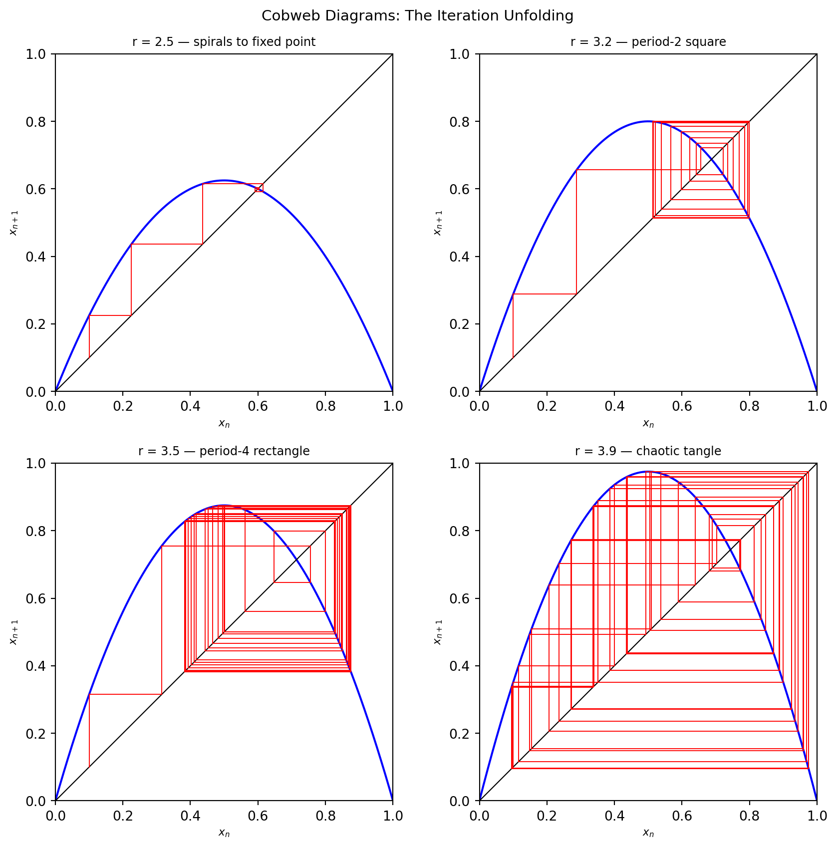
There is a more direct way to *see* these iterations unfold.
A **cobweb diagram** overlays the parabola $y = rx(1-x)$
and the diagonal $y = x$ on the same axes, then traces each
step as a right-angle staircase: move vertically from the
current $x$ up to the parabola (computing $x_{n+1}$), then
move horizontally to the diagonal (making $x_{n+1}$ the
new input), and repeat. The staircase draws the orbit
with every step visible.
### Research Example: Reading the Orbit as a Staircase {.unnumbered .unlisted}
A cobweb diagram traces each iteration as a right-angle staircase on the parabola $y = rx(1-x)$ and the diagonal $y = x$.
Can one picture make the difference between convergence, period-2 cycling, period-4 cycling, and chaos unmistakably visible?
```{python}
# uses: draw_cobweb()
#| label: fig-logistic-cobweb
#| fig-cap: "Cobweb diagrams trace each iteration as a right-angle staircase on the parabola y=rx(1-x) and the diagonal y=x. Top-left: the staircase spirals inward to the fixed point (r=2.5). Top-right: the staircase locks into a square, bouncing between two values (r=3.2). Bottom-left: the staircase settles into a four-cornered rectangle, cycling through four values (r=3.5). Bottom-right: the staircase tangles chaotically across the whole interval (r=3.9)."
import matplotlib.pyplot as plt

def draw_cobweb(ax, r, x0, steps, title):
    xs = [x0]
    x = x0
    for _ in range(steps):
        x = r * x * (1 - x)
        xs.append(x)

    x_grid = [i / 400 for i in range(401)]
    y_parab = [r * xi * (1 - xi) for xi in x_grid]
    ax.plot(x_grid, y_parab, 'b-', lw=1.5)
    ax.plot(x_grid, x_grid,  'k-', lw=0.8)

    x_cur = xs[0]
    for x_next in xs[1:]:
        ax.plot([x_cur, x_cur],   [x_cur, x_next], 'r-', lw=0.7)
        ax.plot([x_cur, x_next], [x_next, x_next], 'r-', lw=0.7)
        x_cur = x_next

    ax.set_xlim(0, 1)
    ax.set_ylim(0, 1)
    ax.set_title(title, fontsize=9)
    ax.set_aspect('equal')
    ax.set_xlabel('$x_n$',    fontsize=8)
    ax.set_ylabel('$x_{n+1}$', fontsize=8)

fig, axes = plt.subplots(2, 2, figsize=(9, 9))
axes = [ax for row in axes for ax in row]

cases = [
    (2.5, 30, 'r = 2.5 — spirals to fixed point'),
    (3.2, 40, 'r = 3.2 — period-2 square'),
    (3.5, 60, 'r = 3.5 — period-4 rectangle'),
    (3.9, 50, 'r = 3.9 — chaotic tangle'),
]
for ax, (r, steps, title) in zip(axes, cases):
    draw_cobweb(ax, r, 0.1, steps, title)

plt.suptitle("Cobweb Diagrams: The Iteration Unfolding", fontsize=11)
plt.tight_layout()
plt.show()
```
The cobweb shapes are unmistakable: a tightening spiral
(converging), a perfect square (period 2), a
four-cornered loop (period 4), and an erratic scribble
(chaos) -- four completely different destinies for the same
equation, determined solely by the growth rate $r$.
## The Bifurcation Diagram {#sec-logistic-bifurcation}
A single plot can summarize all of this behavior at once.
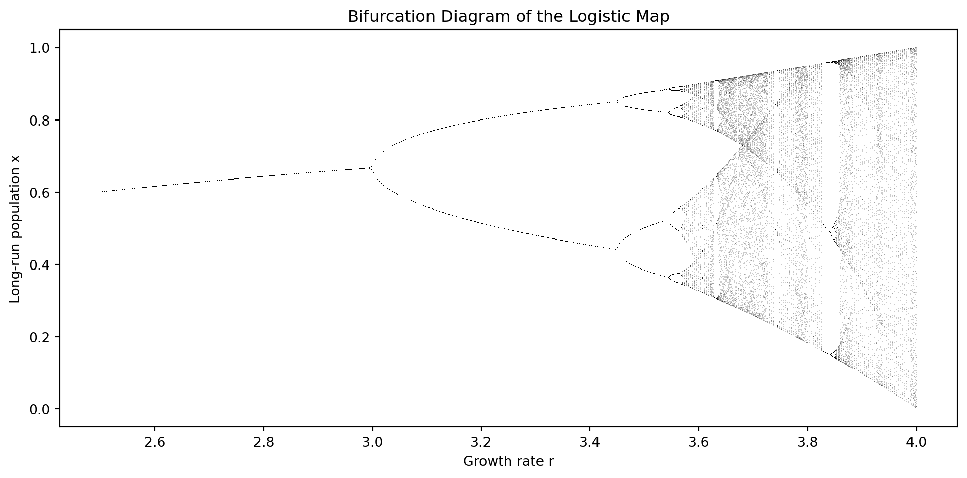
A **bifurcation diagram** shows, for every value of $r$
from 2.5 to 4.0, the set of values that $x_n$ actually
visits after it has settled down -- after the first
several hundred steps (the **transients**) are discarded.
- For $r < 3$: a single dot (one fixed point).
- Near $r = 3$: the line splits into two branches (period 2).
- Near $r \approx 3.449$: each branch splits again (period 4).
- Near $r \approx 3.544$: splits again (period 8).
- Above $r \approx 3.57$: the dots fill a dense cloud (chaos).
We generate this by scanning $r$ from 2.5 to 4.0, running
the map for 500 warmup steps, then plotting the next 200.
### Research Example: One Picture for Every Growth Rate {.unnumbered .unlisted}
Instead of watching one orbit at a time, can we compress the entire behavior of the logistic map into a single image?
We scan $r$ from 2.5 to 4.0, discard 500 warmup steps, and plot the next 200 long-run values for each rate.
```{python}
#| label: fig-logistic-bifurcation
#| fig-cap: "Bifurcation diagram of the logistic map: for each r from 2.5 to 4.0, the long-run population values after discarding 500 transient steps. A single dot means a fixed point; two branches mean period-2; the dense cloud means chaos. Self-similar bifurcation trees are visible inside the chaotic region."
import matplotlib.pyplot as plt

r_min, r_max = 2.5, 4.0
n_r     = 1200   # number of r values to scan
warmup  = 500    # transient steps to discard
collect = 200    # attractor steps to plot

r_vals = [r_min + (r_max - r_min) * i / n_r
          for i in range(n_r + 1)]

r_plot = []
x_plot = []

for r in r_vals:
    x = 0.5
    for _ in range(warmup):
        x = r * x * (1 - x)
    for _ in range(collect):
        x = r * x * (1 - x)
        r_plot.append(r)
        x_plot.append(x)

fig, ax = plt.subplots(figsize=(10, 5))
# ',' draws each point as one pixel -- fast for 240k pts
ax.plot(r_plot, x_plot, ',k', alpha=0.2)
ax.set_xlabel("Growth rate r")
ax.set_ylabel("Long-run population x")
ax.set_title("Bifurcation Diagram of the Logistic Map")
plt.tight_layout()
plt.show()
```
The result is one of the most famous images in mathematics.
Notice the **self-similarity**: each chaotic band contains
its own smaller bifurcation tree, which contains a smaller
tree still, and so on without end. This is a hallmark of
fractal structure -- a theme we will develop further in
Chapter 12.
## Feigenbaum's Constant {#sec-logistic-feigenbaum}
```{python}
#| echo: false
from pathlib import Path; import urllib.request
_d = Path('images'); _d.mkdir(exist_ok=True)
_p = _d / 'mitchell_feigenbaum.jpg'
if not _p.exists():
try:
_req = urllib.request.Request('https://www.rockefeller.edu/news/uploads/www.rockefeller.edu/sites/13/2019/07/Feature_Feigenbaum.jpg', headers={'User-Agent': 'Mozilla/5.0 (educational-book-project)'})
with urllib.request.urlopen(_req) as _resp: _p.write_bytes(_resp.read())
except Exception: pass
```
::: {.content-visible when-format="pdf"}
```{=latex}
\begin{center}
\begin{minipage}[c]{0.22\textwidth}
\includegraphics[width=\textwidth]{images/mitchell_feigenbaum.jpg}
\end{minipage}%
\hspace{0.03\textwidth}%
\begin{minipage}[c]{0.55\textwidth}
\small\textit{Mitchell Feigenbaum (1944--2019)}\\[2pt]
\tiny Photo: \url{https://www.rockefeller.edu/news/26289-mitchell-feigenbaum-physicist-pioneered-chaos-theory-died/}
\end{minipage}
\end{center}
```
:::
::: {.content-visible when-format="html"}
<div style="display:flex; align-items:center; margin:1em 0; gap:12px;">
<img src="images/mitchell_feigenbaum.jpg" style="width:100px; flex-shrink:0;" alt="Mitchell Feigenbaum">
<div style="font-size:0.82em;"><em>Mitchell Feigenbaum (1944–2019)</em><br><span style="font-size:0.85em;">Photo: <a href="https://www.rockefeller.edu/news/26289-mitchell-feigenbaum-physicist-pioneered-chaos-theory-died/">rockefeller.edu</a></span></div>
</div>
:::
Look at the values of $r$ where the period doubles:
$$r_1 = 3, \quad r_2 \approx 3.4495, \quad
r_3 \approx 3.5441, \quad r_4 \approx 3.5644,
\quad r_\infty \approx 3.5699$$
The gaps $r_2 - r_1$, $r_3 - r_2$, $r_4 - r_3$, $\ldots$
shrink geometrically. Their successive ratios converge to
$$\delta = \lim_{n \to \infty}
\frac{r_n - r_{n-1}}{r_{n+1} - r_n} \approx 4.66920\ldots$$
This is **Feigenbaum's constant**, discovered by Mitchell
Feigenbaum in 1978 [@feigenbaum1978].
What makes it astonishing is that the **same constant**
appears in *every* smooth unimodal (single-hump) map --
the logistic map, the sine map $r\sin(\pi x)$, the
cubic map, and thousands of others. No matter the specific
formula, the ratio of consecutive bifurcation gaps always
converges to 4.66920. Feigenbaum had found a universal
law lurking inside chaos.
The value $r_3 = 3.544090\ldots$ listed above is what
Borwein et al. (2006) call $B_3$ in EMA §3.2, where they
compute it to over 1000 digits using high-precision
arithmetic similar to the `mpmath` techniques from
@sec-constants-mpmath [@borwein2006ema, §3.2].
Let us write a function that estimates the period of the
logistic map at a given $r$, then verify the period
transitions with a spot check.
### Research Example: How Fast Does the Cascade Shrink? {.unnumbered .unlisted}
Each period-doubling occurs at a larger $r$ than the last, but the gaps between doublings shrink geometrically.
We first build a period detector, then measure consecutive bifurcation gaps to check whether their ratio is already approaching 4.66920.
```{python}
def orbit_period(r, x0=0.5, warmup=2000,
                 check=64, tol=1e-8):
    """Estimate the period of the orbit at r."""
    x = x0
    for _ in range(warmup):
        x = r * x * (1 - x)
    history = []
    for _ in range(check):
        x = r * x * (1 - x)
        history.append(x)
    for p in [1, 2, 3, 4, 6, 8, 12, 16]:
        ok = all(
            abs(history[j] - history[j + p]) < tol
            for j in range(len(history) - p)
        )
        if ok:
            return p
    return -1    # chaotic or very-high period

tests = [2.8, 3.1, 3.40, 3.46, 3.50,
         3.56, 3.58, 3.65, 3.83]
print(f"{'r':>6}  {'period':>8}")
print("-" * 18)
for r in tests:
    p = orbit_period(r)
    label = str(p) if p > 0 else "chaos"
    print(f"{r:6.2f}  {label:>8}")
```
```{python}
# Feigenbaum ratios from known bifurcation points
# (Borwein et al., EMA 2006, §3.2)
bifu = [3.0, 3.449490, 3.544090, 3.564407]

print("Consecutive bifurcation gap ratios:")
print("-" * 38)
for i in range(1, len(bifu) - 1):
    gap1  = bifu[i]     - bifu[i - 1]
    gap2  = bifu[i + 1] - bifu[i]
    ratio = gap1 / gap2
    print(f"  gap {i} / gap {i+1} = {ratio:.5f}")
print()
print("Converging to delta = 4.66920...")
```
Expected output:
```
Consecutive bifurcation gap ratios:
--------------------------------------
  gap 1 / gap 2 = 4.75148
  gap 2 / gap 3 = 4.65620

Converging to delta = 4.66920...
```
With only two ratios the convergence is already within 2%
of the true value. Each additional bifurcation point
brings the estimate roughly four times closer, because the
convergence rate is exactly $\delta$ itself.
Feigenbaum's constant is not a mathematical curiosity for
physicists alone. It has been measured experimentally in
dripping faucets, oscillating electronic circuits, and
convecting fluids. The same number, 4.669, shows up in
all of them -- a reminder that the abstract map
$x_{n+1} = rx_n(1-x_n)$ is not just a mathematical toy
but a model of how nonlinear systems universally behave
near the transition from order to chaos.
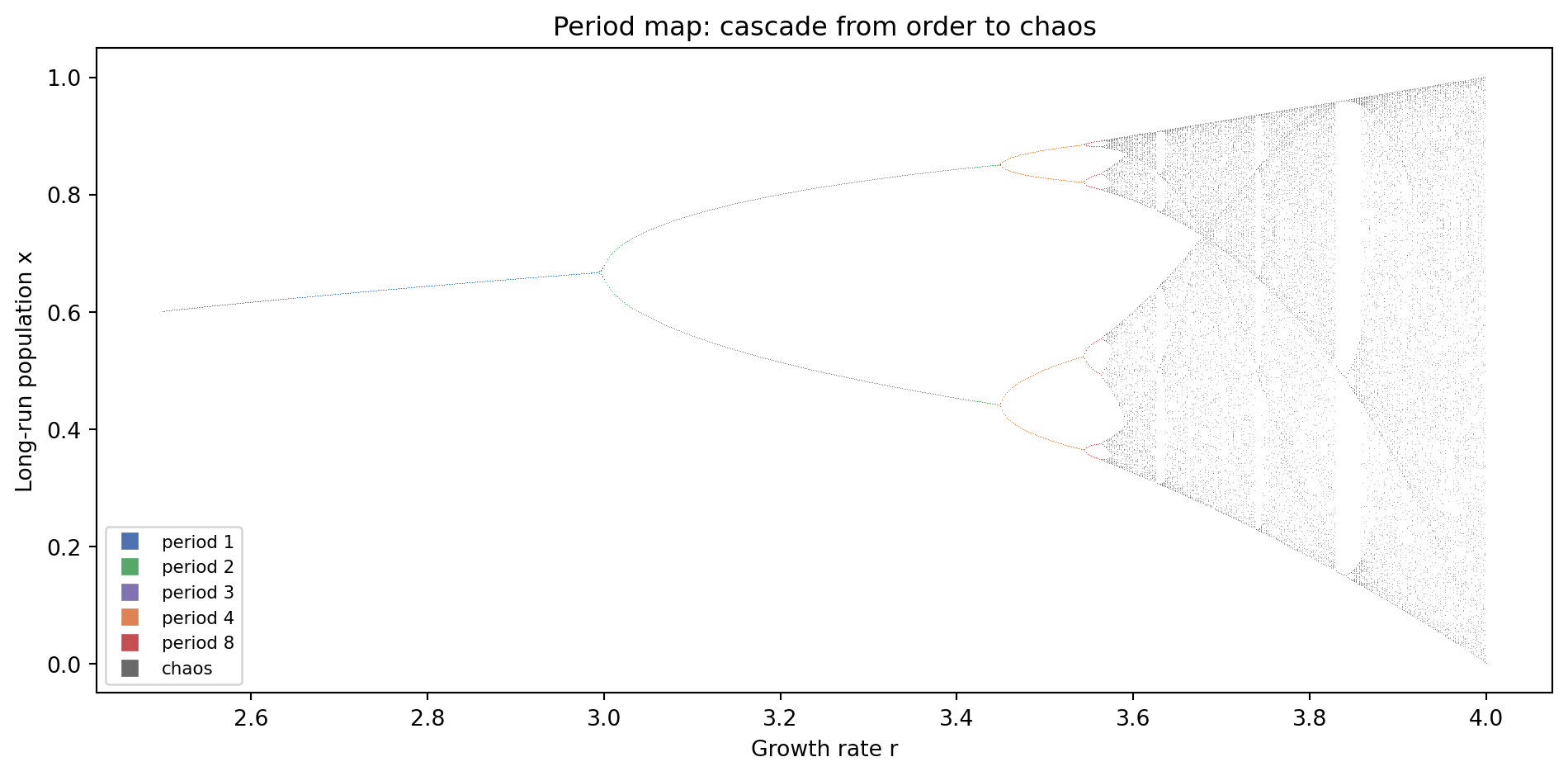
We can make the cascade structure vivid in a single picture
by repainting the bifurcation diagram with a different color
for each period. The result is a **period map**: blue for
the fixed point, green for period 2, orange for period 4,
red for period 8, and gray for chaos. The purple island
near $r \approx 3.83$ is the period-3 window -- we will
zoom into it two sections ahead.
### Research Example: Painting the Cascade by Period {.unnumbered .unlisted}
The monochromatic bifurcation diagram shows *where* orbits live but not which period each point belongs to.
What if we recolor each attractor point by its orbit period, so the Feigenbaum cascade lights up as a sequence of distinct color shifts?
```{python}
#| label: fig-logistic-periodmap
#| fig-cap: "Period map of the logistic map: the bifurcation diagram repainted by orbit period. Blue = fixed point, green = period 2, orange = period 4, red = period 8, purple = period-3 window, gray = chaos. The cascade through blue to red compresses by Feigenbaum's factor before dissolving into gray; the purple island near r ≈ 3.83 is the period-3 window."
# uses: orbit_period()
import matplotlib.pyplot as plt
from matplotlib.lines import Line2D

period_colors = {
    1:  '#4c72b0',
    2:  '#55a868',
    3:  '#8172b2',
    4:  '#dd8452',
    8:  '#c44e52',
    -1: 'dimgray',
}
period_labels = {
    1: 'period 1',
    2: 'period 2',
    3: 'period 3',
    4: 'period 4',
    8: 'period 8',
    -1: 'chaos',
}

r_min, r_max = 2.5, 4.0
n_r     = 800
warmup  = 500
collect = 100

r_vals = [
    r_min + (r_max - r_min) * i / n_r
    for i in range(n_r + 1)
]

fig, ax = plt.subplots(figsize=(10, 5))

for r in r_vals:
    p = orbit_period(r)
    c = period_colors.get(p, 'dimgray')
    x = 0.5
    for _ in range(warmup):
        x = r * x * (1 - x)
    pts = []
    for _ in range(collect):
        x = r * x * (1 - x)
        pts.append(x)
    ax.plot([r] * collect, pts, ',',
            color=c, alpha=0.5)

handles = [
    Line2D(
        [0], [0], color=period_colors[k],
        marker='s', linestyle='None',
        markersize=7, label=period_labels[k]
    )
    for k in [1, 2, 3, 4, 8, -1]
]
ax.legend(handles=handles, fontsize=8,
          loc='lower left')
ax.set_xlabel("Growth rate r")
ax.set_ylabel("Long-run population x")
ax.set_title(
    "Period map: cascade from order to chaos"
)
plt.tight_layout()
plt.show()
```
The color bands snap from blue to green to orange to red as $r$ grows, tracing the period-doubling cascade at a glance.
The purple island near $r \approx 3.83$ interrupts the gray chaos like an oasis of order -- and it contains its own tinier bifurcation tree inside.
## Sensitive Dependence on Initial Conditions {#sec-logistic-chaos}
In the chaotic regime ($r \gtrsim 3.57$), two orbits
starting at almost the same point rapidly diverge.
This is **sensitive dependence on initial conditions** --
colloquially, the **butterfly effect**: a butterfly
flapping its wings in Brazil could, in principle, shift
whether a tornado forms in Texas two weeks later.
The divergence is exponential. If two orbits start at
$x_0$ and $x_0 + \varepsilon$, their separation grows
approximately as $\varepsilon \cdot e^{\lambda n}$, where
$\lambda > 0$ is the **Lyapunov exponent**. A positive
Lyapunov exponent is one standard definition of chaos.
### Research Example: When Does a Tiny Difference Become Everything? {.unnumbered .unlisted}
In a chaotic system, two orbits starting $0.0001$ apart eventually become completely uncorrelated.
How many steps does it take — and is the divergence truly exponential, or does it just look that way?
```{python}
#| label: fig-logistic-chaos
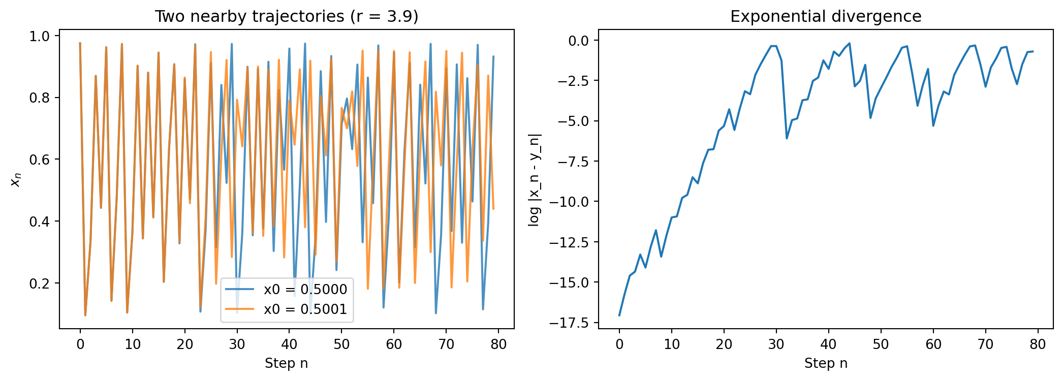
#| fig-cap: "Sensitive dependence: two logistic map trajectories starting 0.0001 apart (x0=0.5000 vs x0=0.5001) at r=3.9. Left: the trajectories are indistinguishable for about 20 steps before diverging completely. Right: log-scale separation rises roughly linearly -- the signature of exponential growth."
import matplotlib.pyplot as plt
import math

r   = 3.9
x0a = 0.5000
x0b = 0.5001     # differs by only 0.0001

steps  = 80
xa, xb = x0a, x0b
xs_a, xs_b, diffs = [], [], []

for _ in range(steps):
    xa = r * xa * (1 - xa)
    xb = r * xb * (1 - xb)
    xs_a.append(xa)
    xs_b.append(xb)
    diffs.append(abs(xa - xb))

fig, axes = plt.subplots(1, 2, figsize=(11, 4))

ax = axes[0]
ax.plot(xs_a, label='x0 = 0.5000', alpha=0.8)
ax.plot(xs_b, label='x0 = 0.5001', alpha=0.8)
ax.set_xlabel("Step n")
ax.set_ylabel("$x_n$")
ax.set_title("Two nearby trajectories (r = 3.9)")
ax.legend()

ax = axes[1]
log_diffs = [
    math.log(d) if d > 1e-15 else -35
    for d in diffs
]
ax.plot(log_diffs)
ax.set_xlabel("Step n")
ax.set_ylabel("log |x_n - y_n|")
ax.set_title("Exponential divergence")

plt.tight_layout()
plt.show()
```
We used `math.log` for the natural logarithm; it was first
introduced at @sec-pascal-dimension.
The two trajectories are indistinguishable for roughly the
first twenty steps, then veer apart and become completely
uncorrelated. The log-separation plot rises roughly as a
straight line -- the hallmark of exponential growth.
This has a deep implication. **Long-range prediction is
impossible in a chaotic system**, not for lack of computing
power, but because any tiny error in the initial measurement
grows without bound. Weather forecasting beyond about
ten to fourteen days faces exactly this mathematical
barrier -- the atmosphere is a high-dimensional chaotic
system, and Feigenbaum's insight explains *why* it cannot
be predicted past a certain horizon, no matter how good
the sensors or the supercomputers.
## Windows of Order {#sec-logistic-windows}
```{python}
#| echo: false
from pathlib import Path; import urllib.request
_d = Path('images'); _d.mkdir(exist_ok=True)
for _fn, _url in [
('ty_li.jpg', 'https://upload.wikimedia.org/wikipedia/commons/1/15/T.Y.Li%2C_2005.jpg'),
('james_yorke.jpg', 'https://upload.wikimedia.org/wikipedia/commons/8/8a/James_A_Yorke.jpg'),
]:
_p = _d / _fn
if not _p.exists():
try:
_req = urllib.request.Request(_url, headers={'User-Agent': 'Mozilla/5.0 (educational-book-project)'})
with urllib.request.urlopen(_req) as _resp: _p.write_bytes(_resp.read())
except Exception: pass
```
::: {.content-visible when-format="pdf"}
```{=latex}
\begin{center}
\begin{minipage}[t]{0.40\textwidth}\centering
\includegraphics[width=0.70\textwidth]{images/ty_li.jpg}\\[4pt]
\small\textit{Tien-Yien Li (1945--2020)}\\[2pt]
\tiny CC BY-SA 4.0, Xw9999, via Wikimedia Commons
\end{minipage}%
\hspace{0.04\textwidth}%
\begin{minipage}[t]{0.40\textwidth}\centering
\includegraphics[width=0.70\textwidth]{images/james_yorke.jpg}\\[4pt]
\small\textit{James A. Yorke (b.\ 1941)}\\[2pt]
\tiny CC BY-SA 3.0, Sijothankam, via Wikimedia Commons
\end{minipage}
\end{center}
```
:::
::: {.content-visible when-format="html"}
<div style="display:flex; justify-content:center; gap:24px; margin:1em 0; flex-wrap:wrap;">
<div style="text-align:center; max-width:160px;">
<img src="images/ty_li.jpg" style="width:120px;" alt="Tien-Yien Li"><br>
<em style="font-size:0.82em;">Tien-Yien Li (1945–2020)</em><br>
<span style="font-size:0.72em;">CC BY-SA 4.0, Xw9999, via Wikimedia Commons</span>
</div>
<div style="text-align:center; max-width:160px;">
<img src="images/james_yorke.jpg" style="width:120px;" alt="James A. Yorke"><br>
<em style="font-size:0.82em;">James A. Yorke (b. 1941)</em><br>
<span style="font-size:0.72em;">CC BY-SA 3.0, Sijothankam, via Wikimedia Commons</span>
</div>
</div>
:::
The bifurcation diagram looks purely chaotic for
$r > 3.57$, but zoom in and you discover surprising
**windows of order** -- narrow ranges of $r$ where
periodic orbits suddenly re-emerge inside the chaos.
The most visible window opens near $r \approx 3.828$,
where a **period-3** orbit appears. In 1975, T. Y. Li
and James Yorke proved a striking theorem: for a continuous
map on an interval, if a period-3 orbit exists, then orbits
of **every other period** also exist -- including periods
5, 7, 11, and all other integers. Their paper was titled
"Period Three Implies Chaos" [@li1975].
The logistic map demonstrates this theorem visually.
Inside the period-3 window the diagram shows exactly three
bands. Just inside the window's right edge those three
bands themselves undergo a full bifurcation cascade --
period 3 splits to period 6, then 12, and so on -- with
its own Feigenbaum scaling.
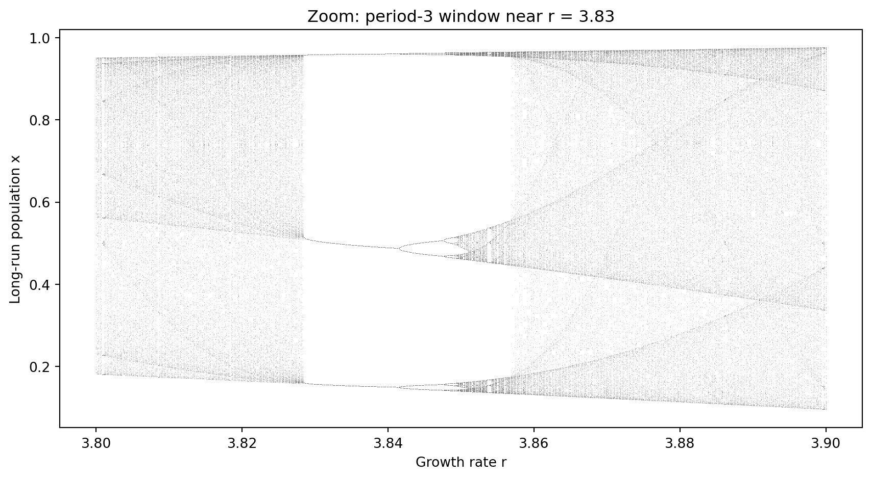
### Research Example: Zooming Into the Period-3 Window {.unnumbered .unlisted}
Inside the apparent chaos near $r \approx 3.83$ hides a narrow island of perfect order: a period-3 orbit.
We zoom into $r \in [3.80, 3.90]$ to expose its own bifurcation structure, then read off the exact three population values the orbit cycles through.
```{python}
#| label: fig-logistic-window
#| fig-cap: "Zoom into the period-3 window near r=3.83: the bifurcation diagram from r=3.80 to r=3.90 reveals three distinct bands that undergo their own period-doubling cascade before returning to chaos at the window's right edge."
import matplotlib.pyplot as plt

# Zoom into the period-3 window
r_min, r_max = 3.80, 3.90
n_r     = 600
warmup  = 800
collect = 300

r_vals = [r_min + (r_max - r_min) * i / n_r
          for i in range(n_r + 1)]

r_plot = []
x_plot = []

for r in r_vals:
    x = 0.5
    for _ in range(warmup):
        x = r * x * (1 - x)
    for _ in range(collect):
        x = r * x * (1 - x)
        r_plot.append(r)
        x_plot.append(x)

fig, ax = plt.subplots(figsize=(9, 5))
ax.plot(r_plot, x_plot, ',k', alpha=0.2)
ax.set_xlabel("Growth rate r")
ax.set_ylabel("Long-run population x")
ax.set_title(
    "Zoom: period-3 window near r = 3.83"
)
plt.tight_layout()
plt.show()
```
```{python}
# uses: orbit_period()
# Confirm period-3 orbit and read off the three values
r = 3.83
print(f"Period at r = {r}: {orbit_period(r)}")

x = 0.5
for _ in range(3000):        # burn in
    x = r * x * (1 - x)

print("\nPeriod-3 attractor values:")
v = []
for _ in range(3):
    x = r * x * (1 - x)
    v.append(x)
    print(f"  {x:.8f}")

# Three more steps should return near v[0]
for _ in range(3):
    x = r * x * (1 - x)
print(f"\nAfter 3 more steps: {x:.8f}")
print(f"Back to v[0]?      {v[0]:.8f}")
```
The output shows exactly three distinct values cycling
endlessly. A hairline shift in $r$ past the window's
boundary shatters the pattern back into featureless chaos.
This interplay between order and chaos is the defining
feature of the logistic map. A purely deterministic rule
with no randomness whatsoever produces behavior that is,
for all practical purposes, unpredictable.
You have seen this theme before: simple rules producing
deep mystery in the Collatz conjecture
(@sec-collatz-rule) and in cellular automata
(@sec-automata-intro). The logistic map adds a new
dimension -- a **continuously tunable parameter** $r$ that
smoothly dials the system from perfectly predictable to
completely chaotic, with the full Feigenbaum cascade in
between.
## The Chaos Meter {#sec-logistic-lyapunov}
The bifurcation diagram shows *where* orbits live, but it
does not tell you *how fast* nearby orbits pull apart.
A single number answers that question: the **Lyapunov
exponent** $\lambda$.
After the transient settles, measure how fast a tiny error
grows. If two orbits start $\varepsilon$ apart, their
separation after $n$ steps is approximately
$\varepsilon \, e^{\lambda n}$. The exponent $\lambda$
is estimated as the average log-slope of the map along the
orbit, where $f'(x) = r(1 - 2x)$ is the slope of the
logistic parabola:
$$\lambda \approx \frac{1}{N} \sum_{n=0}^{N-1}
\ln \bigl| r(1 - 2x_n) \bigr|$$
- $\lambda < 0$: errors *shrink* -- the orbit is stable.
- $\lambda = 0$: right at a bifurcation boundary.
- $\lambda > 0$: errors *grow* -- chaos.
Plotting $\lambda(r)$ across all growth rates produces a
**chaos meter** that shows the exact boundary between order
and chaos. Every window of order inside the chaotic region
shows up as a sudden dip below zero -- including the
period-3 window near $r \approx 3.83$.
### Research Example: A Chaos Meter Across All Growth Rates {.unnumbered .unlisted}
The Lyapunov exponent measures precisely how fast two nearby orbits pull apart — positive means chaos, negative means order.
Can we plot $\lambda(r)$ from $r = 2.5$ to $r = 4.0$ and see a sharp boundary between order and chaos, with every window of order registering as a dip below zero?
```{python}
#| label: fig-logistic-lyapunov
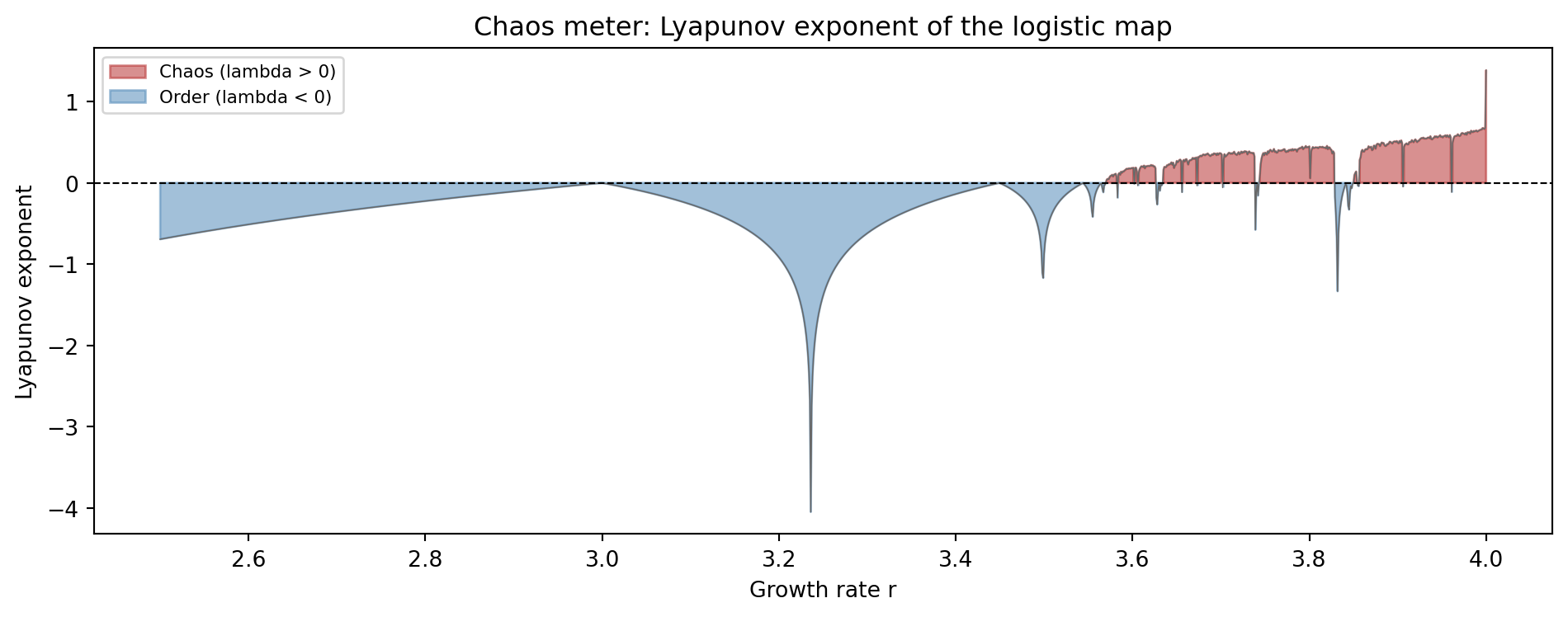
#| fig-cap: "Chaos meter: Lyapunov exponent of the logistic map from r=2.5 to 4.0. Red-shaded regions (lambda>0) are chaotic; blue-shaded regions (lambda<0) are ordered. The dashed line marks lambda=0, the exact chaos boundary. Every window of order -- including the period-3 window near r=3.83 -- shows up as a blue dip inside the red band."
import math
import matplotlib.pyplot as plt

r_min, r_max = 2.5, 4.0
n_r    = 1500
warmup = 500
n_lya  = 1000

r_vals = [
    r_min + (r_max - r_min) * i / n_r
    for i in range(n_r + 1)
]

lya = []
for r in r_vals:
    x = 0.5
    for _ in range(warmup):
        x = r * x * (1 - x)
    total = 0.0
    for _ in range(n_lya):
        x = r * x * (1 - x)
        d = abs(r * (1 - 2 * x))
        total += (
            math.log(d) if d > 0 else -35.0
        )
    lya.append(total / n_lya)

fig, ax = plt.subplots(figsize=(10, 4))
ax.plot(r_vals, lya, color='dimgray', lw=0.6)
ax.fill_between(
    r_vals, lya, 0,
    where=[v >= 0 for v in lya],
    color='firebrick', alpha=0.5,
    label='Chaos (lambda > 0)'
)
ax.fill_between(
    r_vals, lya, 0,
    where=[v < 0 for v in lya],
    color='steelblue', alpha=0.5,
    label='Order (lambda < 0)'
)
ax.axhline(0, color='black', lw=0.8, ls='--')
ax.set_xlabel('Growth rate r')
ax.set_ylabel('Lyapunov exponent')
ax.set_title(
    'Chaos meter: Lyapunov exponent '
    'of the logistic map'
)
ax.legend(fontsize=8)
plt.tight_layout()
plt.show()
```
The dip near $r = 3.83$ is the period-3 window snapping
the chaos back to order. The tall spikes downward
elsewhere each mark a smaller window of periodic behavior
hiding inside the apparent randomness. Every bifurcation
point -- $r \approx 3$, $r \approx 3.449$,
$r \approx 3.544$, and so on -- appears precisely as
$\lambda = 0$: the exact boundary between stability and
divergence.
At $r = 4$ the Lyapunov exponent reaches its maximum of
$\ln 2 \approx 0.693$, a fact provable analytically using
the **arcsine density** $\rho(x) = 1/(\pi\sqrt{x(1-x)})$.
Even at peak chaos, mathematics dictates where the orbit
spends its time -- most near $x = 0$ and $x = 1$, least
near the middle. We can verify this directly:
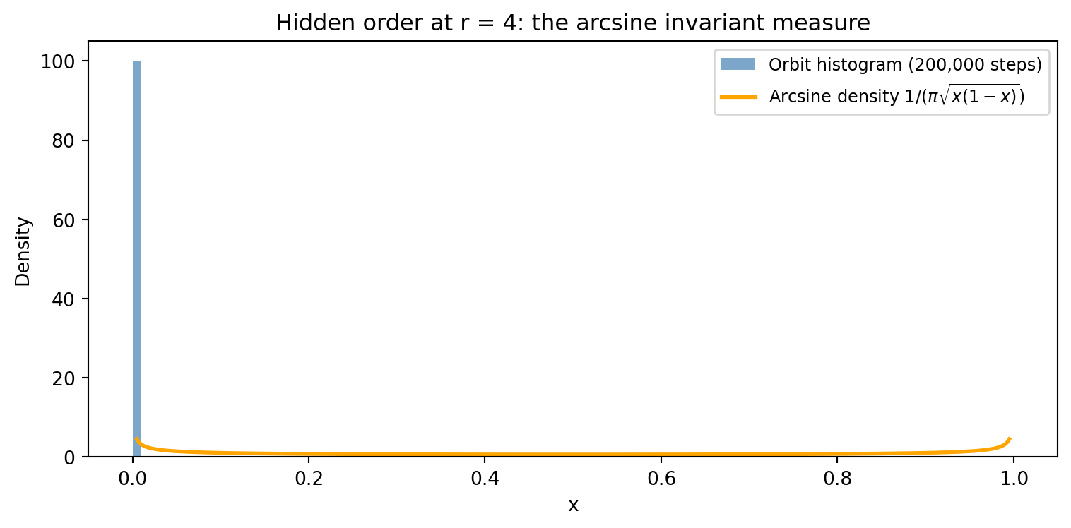
### Research Example: Does Chaos Obey a Law? {.unnumbered .unlisted}
Even at maximum chaos ($r = 4$), the logistic map spends more time near $x = 0$ and $x = 1$ than near the middle — by a precise mathematical formula.
We run 200,000 steps and overlay the theoretical arcsine density to see whether a quarter-million-step orbit matches the prediction.
```{python}
#| label: fig-logistic-arcsine
#| fig-cap: "Hidden order at maximum chaos: the logistic map at r=4 visits different regions at unequal rates. The orbit histogram (200,000 steps) matches the arcsine density exactly — highest near x=0 and x=1, lowest near x=0.5. Even peak chaos obeys a precise mathematical distribution."
import math
import matplotlib.pyplot as plt

r_arc = 4.0
x_arc = 0.5
xs_arc = []
for _ in range(200_000):
    x_arc = r_arc * x_arc * (1 - x_arc)
    xs_arc.append(x_arc)

fig, ax = plt.subplots(figsize=(8, 4))
ax.hist(xs_arc, bins=100, density=True,
        color='steelblue', alpha=0.7,
        label='Orbit histogram (200,000 steps)')

x_grid = [0.005 + 0.99 * i / 499 for i in range(500)]
rho    = [1.0 / (math.pi * math.sqrt(xi * (1 - xi)))
          for xi in x_grid]
ax.plot(x_grid, rho, color='orange', lw=2,
        label=r'Arcsine density $1/(\pi\sqrt{x(1-x)})$')

ax.set_xlabel("x")
ax.set_ylabel("Density")
ax.set_title("Hidden order at r = 4: the arcsine invariant measure")
ax.legend(fontsize=9)
plt.tight_layout()
plt.show()
```
The U-shaped curve is the theoretical prediction; the
histogram is a purely numerical experiment. They agree
exactly -- a reminder that even total chaos has hidden
mathematical structure.
## Further Research Topics {#sec-logistic-research}
1. **Cobweb diagrams.** A cobweb diagram overlays the
parabola $y = rx(1-x)$ and the diagonal $y = x$, then
traces each iteration as a staircase: move vertically to
the parabola, then horizontally to the diagonal, repeat.
Implement `cobweb(r, x0, steps)` in Python and plot the
diagram for $r = 2.5$ (converging), $r = 3.2$ (period 2),
$r = 3.5$ (period 4), and $r = 3.9$ (chaotic). Describe
how the visual shape of the staircase changes across these
four cases.
*(Problem proposed by Claude Code.)*
2. **Stability of the fixed point.** The fixed point
$x^* = 1 - 1/r$ is stable when $|f'(x^*)| < 1$, where
$f'(x) = r(1 - 2x)$ is the derivative of the logistic
map. Substitute $x^*$ to show that stability requires
$1 < r < 3$. Verify this numerically: for each $r$
in $\{1.5, 2.0, 2.5, 2.9, 3.0, 3.1\}$, start at
$x_0 = x^* + 0.1$ (slightly off the fixed point) and
run 100 iterations. Does the orbit converge or diverge?
*(Problem proposed by Claude Code.)*
3. **Period-doubling in other maps.** Feigenbaum's constant [@feigenbaum1978]
is universal. Investigate the **sine map**
$x_{n+1} = r\sin(\pi x_n)$ (domain $[0,1]$,
$r \in [0,1]$) and the **tent map**
$x_{n+1} = r x_n$ if $x_n \le 0.5$ else
$r(1-x_n)$. Compute the first three bifurcation points
of each map using the `orbit_period` approach from this
chapter. Are the consecutive gap ratios approaching
4.66920?
*(Problem proposed by Claude Code.)*
4. **Lyapunov exponents.** The Lyapunov exponent at
growth rate $r$ can be estimated as
$\lambda \approx \frac{1}{N}\sum_{n=0}^{N-1}
\ln|r(1-2x_n)|$.
(We used `math.log` for natural logarithm at
@sec-pascal-dimension.)
Compute $\lambda$ for $r$ from 2.5 to 4.0 and plot it
alongside the bifurcation diagram. Where is
$\lambda > 0$? Where is $\lambda < 0$? What happens
at the period-3 window at $r \approx 3.83$?
*(Problem proposed by Claude Code.)*
5. **Predicting the accumulation point.** The chaos
onset $r_\infty \approx 3.5699946$ can be estimated
by Feigenbaum's convergence formula
$r_\infty \approx r_n + C / \delta^n$, where $C$ is a
constant and $\delta = 4.66920$. Using the four known
bifurcation points from this chapter, fit $C$ by
least squares and predict $r_5$ and $r_6$. How close
is your predicted $r_\infty$ to the known value?
*(Problem proposed by Claude Code.)*
6. **The period-3 window in detail.** Inside the period-3
window the orbit undergoes its own bifurcation cascade:
period 3 splits to period 6, then 12, and so on.
Zoom your bifurcation diagram into
$r \in [3.855, 3.858]$ using $n_r = 2000$ and
$\text{warmup} = 1000$. Measure the two consecutive
bifurcation gaps inside this secondary cascade. Is the
ratio again approaching 4.66920, or is it different?
*(Problem proposed by Claude Code.)*
7. **Chaos and binary digits.** At $r = 4$ (fully
chaotic), the logistic map is exactly conjugate to the
**doubling map** $\theta_{n+1} = 2\theta_n \pmod 1$
via $x_n = \sin^2(\pi\theta_n)$. The doubling map
shifts the binary digits of $\theta_0$ one place left
at each step (see @sec-modular-operator). This means
the entire future of $x_n$ is encoded in the binary
digits of $\theta_0$. Start with $\theta_0 = 1/3$
(binary $0.\overline{01}$, period 2) and verify that
$x_n$ is periodic. Now start with $\theta_0 = \pi/4$
and check whether the orbit appears periodic.
*(Problem proposed by Claude Code.)*
8. **The logistic map as a pseudorandom generator.** At
$r = 3.9$, threshold the orbit: output 1 if $x_n > 0.5$,
else 0. Apply two statistical tests from
@sec-constants-normal (frequency test and runs test) to
the resulting bit sequence of length 10,000. Does the
logistic map pass these tests? Compare to a true
pseudorandom sequence from `random.randint(0, 1)` (first
used at @sec-automata-symmetry).
*(Problem proposed by Claude Code.)*
9. **The Hénon map** [@henon1976]**.** The **Hénon map** is a 2D
generalization:
$x_{n+1} = 1 - ax_n^2 + y_n$,
$y_{n+1} = bx_n$.
For $a = 1.4$, $b = 0.3$, the long-run attractor is a
fractal called the **Hénon strange attractor**. Plot
100,000 iterates as $(x_n, y_n)$ points using
`ax.plot(xs, ys, ',k', alpha=0.3)`.
Describe the structure: how many "sheets" does it
appear to have? How does it compare to the bifurcation
diagram?
*(Problem proposed by Claude Code.)*
10. **Measuring the Feigenbaum constant numerically.**
The orbit-period method of this chapter detects integer
periods but cannot find high-period (e.g. period-32)
orbits. Design a more robust bifurcation-point finder:
run the map for 5000 warmup steps and 512 collect steps;
count distinct values in the orbit to tolerance $10^{-6}$.
Use binary search to locate $r_5$ (where period changes
from 16 to 32) to 6 decimal places. Compute the
third Feigenbaum ratio and compare to 4.66920.
*(Problem proposed by Claude Code.)*
11. **Universality class and the quadratic maximum.**
Feigenbaum's universality applies to all maps with a
single smooth maximum of the form $f(x) \sim c - |x|^z$
near the top, **only when $z = 2$** (quadratic max).
A map with a cubic maximum ($z = 3$) has a different
Feigenbaum constant, approximately 4.6651. Investigate
the map $x_{n+1} = r(1 - |2x_n - 1|^3)$ (a cubic-max
analogue on $[0,1]$). Compute the first three
bifurcation points and estimate the gap ratio. Is it
closer to 4.6692 or 4.6651?
*(Problem proposed by Claude Code.)*
12. **Chaos in continuous time: the Lorenz system.**
The logistic map is a discrete-time chaotic system.
In 1963, Edward Lorenz discovered [@lorenz1963] that a set of three
coupled differential equations
$\dot{x} = \sigma(y-x)$,
$\dot{y} = x(\rho - z) - y$,
$\dot{z} = xy - \beta z$
also exhibits sensitive dependence and a fractal
attractor (the **Lorenz butterfly**). Using Python's
`scipy.integrate.odeint` (look up the documentation),
integrate the Lorenz system with $\sigma=10$,
$\rho=28$, $\beta=8/3$ and plot the trajectory in 3D.
Identify the two "lobes" of the butterfly and describe
how the orbit switches between them unpredictably.
*(Problem proposed by Claude Code.)*
13. **Symbolic dynamics and itineraries.** Label each
orbit point $L$ if $x_n < 0.5$ and $R$ if $x_n > 0.5$.
The resulting infinite string is the **itinerary** of
the orbit. For periodic orbits the itinerary is a
repeating block (e.g., $LR$ for period 2, $LLR$ for
period 3). Write code that extracts the itinerary
of any orbit. Show that the period-3 orbit at
$r = 3.83$ has itinerary $LLR$ (or one of its cyclic
rotations). Research **kneading theory** [@milnorthurston1977] to see how itineraries classify all
possible orbit types. What itinerary would a
period-5 orbit in the smallest period-5 window have?
*(Problem proposed by Claude Code.)*
14. **Sharkovsky's theorem: period 3 forces everything.**
In 1964, Oleksandr Sharkovsky [@sharkovsky1964] proved that for any
continuous map on a closed interval, the periods that
can coexist follow a strict ordering:
$3 \succ 5 \succ 7 \succ \cdots \succ 6 \succ 10
\succ \cdots \succ 4 \succ 2 \succ 1$.
If a map has any orbit of period $m$, it also has orbits
of every period to the right of $m$ in this list.
In particular, period 3 forces orbits of *every* period
to coexist somewhere -- a result publicized in the West
by @li1975 as "Period Three Implies Chaos."
Verify this numerically: at $r = 3.83$ (inside the
period-3 window), the default orbit from $x_0 = 0.5$
has period 3. Now scan starting points
$x_0 \in \{0.1, 0.15, 0.2, \ldots, 0.95\}$ using the
`orbit_period` function (extended to detect up to
period 24) and collect all distinct periods found.
Do you find periods other than 3? Which ones? This
is qualitatively different from kneading theory
(topic 13), which classifies the *structure* of an
orbit; Sharkovsky's theorem tells you which *periods*
must coexist whenever a given period is present.
*(Problem proposed by Claude Code.)*
15. **Float precision and the sensitivity of chaos.**
At $r = 4$, the logistic map has Lyapunov exponent
$\lambda = \ln 2$, so small errors double every step.
A Python `float` has about 16 decimal digits of
precision; `mpmath` (used in @sec-constants-mpmath)
can carry 50 digits. Start both at $x_0 = 0.3$ and
run them in parallel:
```python
from mpmath import mp, mpf
mp.dps = 50
x_mp = mpf('0.3')
x_fl = 0.3
for n in range(1, 200):
    x_mp = 4 * x_mp * (1 - x_mp)
    x_fl = 4.0 * x_fl * (1.0 - x_fl)
    if abs(float(x_mp) - x_fl) > 0.01:
        print(f"Diverged at step {n}")
        break
```
At what step do they diverge by more than 0.01?
Does the answer change if you use $x_0 = 0.1$ or
$x_0 = 0.7$? The Lyapunov exponent predicts that
a precision gap of $\Delta_0$ grows to $\Delta_0 e^{\lambda n}$
after $n$ steps; use this to estimate the divergence
step from the initial digit gap, and compare to what
you observe. Now try $r = 3.5$ (inside a stable
period-4 window) -- does the divergence happen faster
or slower, and why?
*(Problem proposed by Claude Code.)*
16. **The Mandelbrot set along the real axis.**
The logistic map $x \mapsto rx(1-x)$ and the quadratic
family $z \mapsto z^2 + c$ (whose filled Julia sets
make the Mandelbrot set of Chapter 12) are the same
dynamical system in disguise. The change of variables
$y_n = r/2 - rx_n$ converts the logistic map to
$y_{n+1} = y_n^2 + c$ with $c = r/2 - r^2/4$.
This formula maps the logistic period-doubling cascade
to points on the *negative real axis* of the
Mandelbrot set.
Use it to convert the four bifurcation points from
this chapter ($r_1 \approx 3$, $r_2 \approx 3.449$,
$r_3 \approx 3.544$, $r_4 \approx 3.565$) into
corresponding $c$ values. For example:
$r = 3 \to c = -0.75$ and
$r_\infty \approx 3.5699 \to c_\infty \approx -1.401$.
Look up the main cardioid and period-2 bulb boundaries
of the Mandelbrot set ($c = -0.75$ is exactly the
junction between them). What does this tell you about
the large black regions of the Mandelbrot set in
Chapter 12?
*(Problem proposed by Claude Code.)*
17. **Invariant density away from $r = 4$.**
At $r = 4$ (see @sec-logistic-lyapunov), the long-run
fraction of time the orbit spends near $x$ follows the
arcsine density $\rho(x) = 1/(\pi\sqrt{x(1-x)})$.
For *other* chaotic values of $r$ the invariant
density is generally *not* arcsine.
Run 200,000 steps of the logistic map for each of
$r \in \{3.7,\, 3.8,\, 3.9,\, 4.0\}$ and plot
normalized histograms (100 bins) on the same axes.
Overlay the arcsine curve only for $r = 4$.
Which values of $r$ produce histograms that look
roughly arcsine? Which look flat? Which have
conspicuous gaps (these correspond to windows of
periodic behavior just below your chosen $r$)?
At $r = 3.7$, use the Lyapunov exponent
(topic 4 formula) to confirm the orbit is genuinely
chaotic before trusting the histogram.
*(Problem proposed by Claude Code.)*
18. **Bifurcation diagram of the Henon map.**
Topic 9 plotted the 2D Hénon attractor at a fixed
parameter pair. Now build a *bifurcation diagram*
for the Henon map by treating $a$ as the variable
parameter (fix $b = 0.3$, scan $a$ from 0.5 to 1.5):
```python
import numpy as np
import matplotlib.pyplot as plt
a_vals = np.linspace(0.5, 1.5, 800)
for a in a_vals:
    x, y = 0.1, 0.1
    for _ in range(2000):           # warmup
        x, y = 1 - a*x*x + y, 0.3*x
    for _ in range(200):            # collect
        x, y = 1 - a*x*x + y, 0.3*x
        plt.plot(a, x, ',k', alpha=0.1, ms=0.5)
```
Compare the resulting diagram to the logistic
bifurcation diagram: does the Henon map also exhibit
a period-doubling cascade? Identify the approximate
$a$ values of the first three bifurcations.
Compute the two consecutive gap ratios and check
whether they approach Feigenbaum's constant 4.66920.
*(Problem proposed by Claude Code.)*
19. **Topological entropy via itinerary counting.**
Building on the $L/R$ itinerary coding of topic 13,
the **topological entropy** of the logistic map at
parameter $r$ can be estimated by counting how many
*distinct* itinerary words of length $n$ appear
across all orbits:
```python
import math
def top_entropy(r, n, n_starts=2000):
    words = set()
    for k in range(n_starts):
        x = (k + 0.5) / n_starts
        word = []
        for _ in range(n):
            x = r * x * (1 - x)
            word.append('R' if x > 0.5 else 'L')
        words.add(tuple(word))
    return math.log(len(words)) / n
```
Compute `top_entropy(r=4, n)` for
$n \in \{5, 10, 15, 20\}$. Does it converge to
$\ln 2 \approx 0.6931$? (At $r = 4$ it can be shown
analytically that all $2^n$ words are realised, so
entropy $= \ln 2$.) Now compute it for
$r \in \{3.7, 3.8, 3.9, 4.0\}$ at $n = 20$. Is the
entropy an increasing function of $r$? What does
the entropy equal inside a periodic window
(try $r = 3.83$)? Compare your entropy estimates
to the Lyapunov exponent at the same $r$ values
(topic 4) -- are they equal?
*(Problem proposed by Claude Code.)*