4 Number Bases

In the Introduction we glimpsed Carl Sagan’s vision: a circle encoded in the digits of $\pi$, but only when those digits are written in base 11. Strip away base 10 and the circle appears. That image raises an immediate question: what is a base, and why would changing it reveal something that was hidden before?

The answer is that a base is nothing more than a choice of alphabet for writing numbers. The number fourteen is the same quantity whether we write 14 (base 10), 1110 (base 2), or E (base 16). The quantity is fixed; the representation is a convention. Digit patterns — palindromes, repeated digits, beautiful symmetries — live in the representation. Some patterns are base-dependent accidents; others reflect deeper arithmetic structure that shows up no matter how you write the number. Learning to tell the difference is one of the skills this chapter develops.

4.1 Positional Notation and Base Conversion

In base $b$, a string of digits $d_{n-1} d_{n-2} \cdots d_1 d_0$ means

\[d_{n-1} \cdot b^{n-1} + d_{n-2} \cdot b^{n-2} + \cdots + d_1 \cdot b^1 + d_0 \cdot b^0.\]

Each position is worth $b$ times the position to its right. In base 10 the positions are ones, tens, hundreds, thousands. In base 2 they are ones, twos, fours, eights, sixteens. In base 16 they are ones, sixteens, two-fifty-sixes.

Python has built-in functions for the three most common non-decimal bases.

n = 255
print(f"Decimal: {n}")
print(f"Binary:  {bin(n)}")    # prefix '0b'
print(f"Octal:   {oct(n)}")    # prefix '0o'
print(f"Hex:     {hex(n)}")    # prefix '0x'

Decimal: 255
Binary:  0b11111111
Octal:   0o377
Hex:     0xff

The 0b, 0o, and 0x prefixes are Python’s notation — the number itself is still 255 in all four lines. Hexadecimal needs six symbols beyond the usual 0-9, so it borrows the letters a-f: a=10, b=11, c=12, d=13, e=14, f=15. Thus 0xff = $15 \cdot 16 + 15 = 255$.

To convert to an arbitrary base $b$ we repeatedly divide by $b$ and collect remainders from bottom to top.

def to_base(n, b):
    """Convert non-negative integer n to base b (2-36)."""
    if n == 0:
        return "0"
    digits = []
    while n:
        digits.append(int(n % b))
        n //= b
    # digits are collected least-significant first
    chars = "0123456789abcdefghijklmnopqrstuvwxyz"
    return "".join(chars[d] for d in reversed(digits))

for base in [2, 8, 11, 16]:
    print(f"255 in base {base:2d}: {to_base(255, base)}")

255 in base  2: 11111111
255 in base  8: 377
255 in base 11: 212
255 in base 16: ff

Base 11 uses the digit a for ten. The string 212 in base 11 means $2 \cdot 121 + 1 \cdot 11 + 2 = 255$.

Going the other way — from a base-$b$ string back to an integer — uses Python’s built-in int(s, base).

# Convert a base-b string back to decimal
print(int("11111111", 2))    # 255 in binary
print(int("ff",      16))    # 255 in hex
print(int("212",     11))    # 255 in base 11

255
255
255

All three return 255. These two functions — to_base and int(s, b) — are the whole conversion toolkit. Every experiment in this chapter uses them.

4.2 Digital Roots: Modular Arithmetic in Disguise

Add the digits of 493: $4 + 9 + 3 = 16$. Add again: $1 + 6 = 7$. That final single digit, 7, is the digital root of 493. The process always terminates because the digit sum of any positive integer is strictly smaller than the integer itself (for $n \geq 10$).

Why does it terminate at a single digit? More interestingly: is there a shortcut?

def digital_root(n):
    while n >= 10:
        n = sum(int(d) for d in str(n))
    return n

samples = [493, 1729, 99999, 100000, 12345]
for n in samples:
    print(f"digital_root({n}) = {digital_root(n)}")

digital_root(493) = 7
digital_root(1729) = 1
digital_root(99999) = 9
digital_root(100000) = 1
digital_root(12345) = 6

The shortcut is a theorem connecting digital roots to modular arithmetic (which we studied in Chapter 2).

Theorem. For any positive integer $n$, $\text{dr}(n) = 1 + (n-1) \bmod 9$. Equivalently: $\text{dr}(n) = n \bmod 9$, unless $9 \mid n$, in which case $\text{dr}(n) = 9$.

The reason is that $10 \equiv 1 \pmod 9$, so $10^k \equiv 1 \pmod 9$ for every $k$. Therefore the value of a number and the sum of its base-10 digits differ by a multiple of 9. Repeatedly summing digits strips away multiples of 9 until only the remainder survives.

# Verify: digital_root(n) equals 1 + (n-1) % 9
def dr_formula(n):
    return 1 + (n - 1) % 9

all_match = all(
    digital_root(n) == dr_formula(n)
    for n in range(1, 10000)
)
print(f"Formula matches digit sum for 1..9999: {all_match}")

Formula matches digit sum for 1..9999: True

In base $b$ the same argument applies, but now the shortcut is mod $(b-1)$ instead of mod 9. In base 16, $\text{dr}(n) = n \bmod 15$ (with the exception that multiples of 15 have digital root 15, written f in hex).

def digital_root_base(n, b):
    while n >= b:
        n = sum(int(d, b) for d in to_base(n, b))
    return n

def dr_formula_base(n, b):
    return 1 + (n - 1) % (b - 1)

# Verify for base 16, n in 1..999
ok = all(
    digital_root_base(n, 16) == dr_formula_base(n, 16)
    for n in range(1, 1000)
)
print(f"Base-16 formula matches for 1..999: {ok}")

Base-16 formula matches for 1..999: True

“Casting out nines” — the old mental arithmetic trick for checking multiplication by verifying digit sums — is exactly this theorem in action. $47 \times 58 = 2726$. Digital root of 47 is 2; digital root of 58 is 4; product $2 \times 4 = 8$; digital root of 2726 is $2+7+2+6 = 17 \to 8$. Check. The trick works in any base: casting out $(b-1)$s.

Research Example: The Nine-Color Quilt of Digital Roots

If digital roots in base 10 always cycle through 1–9, what does that look like when you lay the first hundred integers side by side — is the cycling perfectly uniform, or does some hidden structure appear?

# uses: digital_root()
import matplotlib.pyplot as plt
import matplotlib.colors as mcolors
import numpy as np

roots = [digital_root(n) for n in range(1, 101)]
grid  = np.array(roots).reshape(10, 10)

tab_colors = list(plt.cm.tab10.colors[:9])
cmap_dr = mcolors.ListedColormap(tab_colors)
norm_dr = mcolors.BoundaryNorm([i + 0.5 for i in range(10)], 9)

fig, ax = plt.subplots(figsize=(7, 7))
im = ax.imshow(grid, cmap=cmap_dr, norm=norm_dr, aspect='equal',
               interpolation='nearest')
for i in range(10):
    for j in range(10):
        dr = roots[i * 10 + j]
        r, g, b = tab_colors[dr - 1][:3]
        txt_color = 'black' if 0.299*r + 0.587*g + 0.114*b > 0.5 else 'white'
        ax.text(j, i, str(10 * i + j + 1), ha='center', va='center',
                fontsize=8, color=txt_color)

cbar = fig.colorbar(im, ax=ax, ticks=range(1, 10), shrink=0.85)
cbar.set_label('Digital Root', fontsize=11)
ax.set_xticks([])
ax.set_yticks([])
ax.set_title('Digital Roots of 1–100: Counting to Nine, Over and Over',
             fontsize=12)
plt.tight_layout()
plt.show()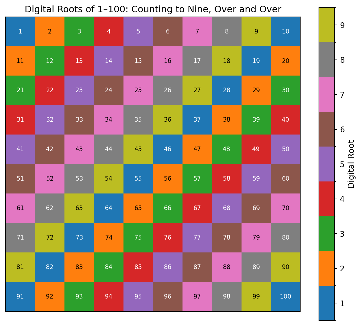

Figure 4.1: Digital roots of 1–100 arranged in a 10×10 grid. Each cell is colored by its digital root (1–9); the number itself is printed inside. Every row shifts the color sequence by one position — the diagonal stripes reveal the repeating mod-9 rhythm underneath ordinary counting.

The diagonal color stripes show that numbers 9 apart always share the same digital root — the quilt tiles perfectly every nine steps. What looks like random color is actually a rigid mod-9 lattice hiding inside the ordinary sequence 1, 2, 3, ….

4.3 Palindromic Numbers Across Bases

A palindrome is a string that reads the same forwards and backwards. The number 121 is a palindrome in base 10. The number 33 in base 10 equals 100001 in base 2 — not a palindrome there. But 9 in base 10 equals 1001 in base 2 — a palindrome in both.

# uses: to_base()
def is_palindrome(n, b):
    s = to_base(n, b)
    return s == s[::-1]

# Numbers that are palindromes in both base 2 and base 10
dual = [
    n for n in range(1, 500)
    if is_palindrome(n, 10) and is_palindrome(n, 2)
]
print("Palindromes in base 2 and base 10 (1-499):")
print(dual)

Palindromes in base 2 and base 10 (1-499):
[1, 3, 5, 7, 9, 33, 99, 313]

The sequence starts 1, 3, 5, 7, 9, 33, 99, 313, 585, … Whether this sequence is infinite is an open question — no proof exists either way.

What about palindromes in three bases simultaneously?

triple = [
    n for n in range(1, 10000)
    if is_palindrome(n, 2)
    and is_palindrome(n, 10)
    and is_palindrome(n, 16)
]
print("Palindrome in bases 2, 10, and 16 (1-9999):")
print(triple)

Palindrome in bases 2, 10, and 16 (1-9999):
[1, 3, 5, 7, 9]

The first interesting multi-base palindrome is 1 (trivially a single digit in every base). The next is a (=10), which is palindromic in base 10 as the single digit a — wait, that is only one digit, so trivially palindromic. Multi-digit palindromes in several bases simultaneously are rare.

Every single-digit number is trivially palindromic in any base larger than it. The interesting cases start when the number has at least two digits in every base we care about.

# Require at least 2 digits in all three bases
non_trivial = [
    n for n in range(4, 100000)
    if len(to_base(n, 2))  >= 2
    and len(to_base(n, 10)) >= 2
    and len(to_base(n, 16)) >= 2
    and is_palindrome(n, 2)
    and is_palindrome(n, 10)
    and is_palindrome(n, 16)
]
print("Non-trivial base-2/10/16 palindromes under 100k:")
print(non_trivial)

Non-trivial base-2/10/16 palindromes under 100k:
[]

Research Example: Where Do Multi-Base Palindromes Hide?

Which numbers below 1500 are multi-digit palindromes in many bases simultaneously — and do they cluster in patterns, or scatter at random?

# uses: to_base(), is_palindrome()
import matplotlib.pyplot as plt

xs_pal, ys_pal = [], []
for n_pal in range(1, 1501):
    for b_pal in range(2, 17):
        s_pal = to_base(n_pal, b_pal)
        if len(s_pal) >= 2 and s_pal == s_pal[::-1]:
            xs_pal.append(n_pal)
            ys_pal.append(b_pal)

fig, ax = plt.subplots(figsize=(11, 4.5))
sc = ax.scatter(xs_pal, ys_pal, c=ys_pal, cmap='viridis', s=5, alpha=0.8, linewidths=0)
cb = fig.colorbar(sc, ax=ax, shrink=0.9)
cb.set_label('Base', fontsize=10)
ax.set_yticks(list(range(2, 17)))
ax.set_xlabel('n', fontsize=12)
ax.set_ylabel('Base', fontsize=12)
ax.set_title(
    'Palindrome Constellation: Multi-Digit Palindromes, n = 1 to 1500',
    fontsize=12
)
plt.tight_layout()
plt.show()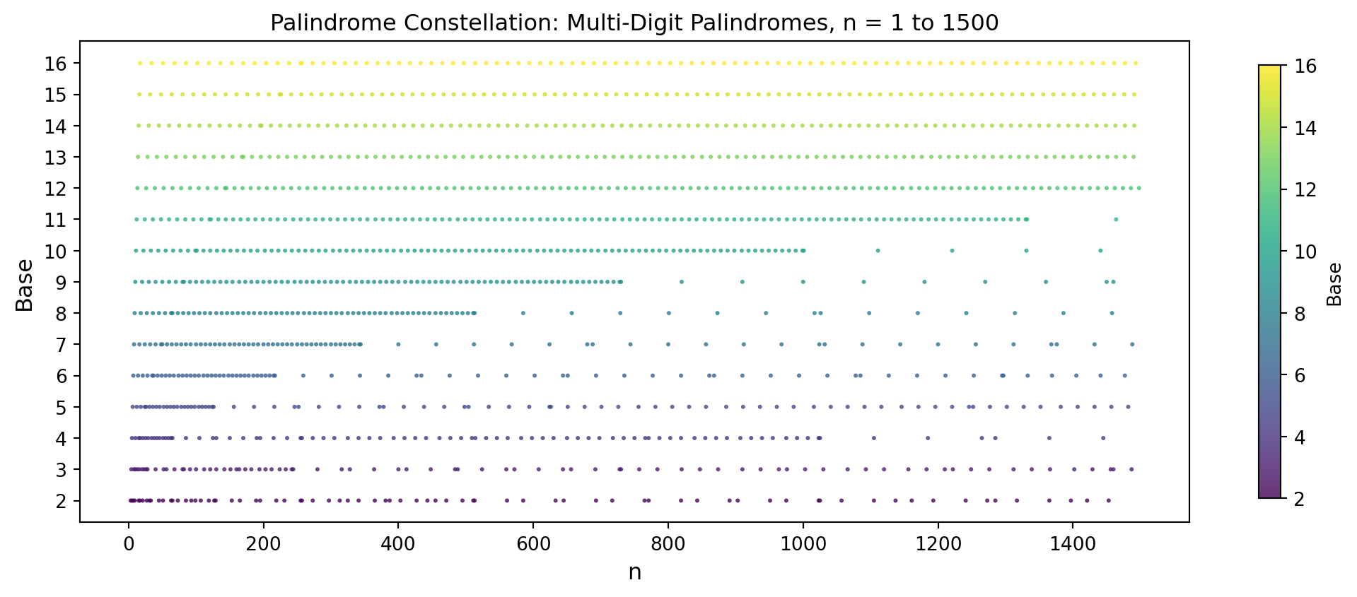

Figure 4.2: Each dot marks a number n (x-axis) that is a multi-digit palindrome in the given base (y-axis) — single-digit trivial cases excluded. Base-2 palindromes (bottom row) are sparse; they occur only for special binary patterns such as 1001 or 10101. Base-16 palindromes (top) are moderately dense: two-digit hex palindromes such as 0x11=17, 0x22=34, … form the evenly-spaced vertical stripes. Most numbers across most bases simply are not palindromes at all.

Base-16 fills the map densely because every two-digit hex number of the form dd (like 0x11 = 17, 0x22 = 34, …) is automatically a palindrome, giving the evenly-spaced stripes. Base-2 is nearly empty — binary palindromes like 1001 and 10101 are rare special cases. You just mapped hidden palindrome structure across fifteen bases at once: that is how computational exploration begins.

4.4 Armstrong Numbers

An Armstrong number (also called a narcissistic number) in base 10 is a number equal to the sum of its own digits each raised to the power equal to the number of digits. The three-digit Armstrong numbers satisfy

\[\overline{abc} = a^3 + b^3 + c^3.\]

For example, $153 = 1^3 + 5^3 + 3^3 = 1 + 125 + 27 = 153$.

# uses: to_base()
def is_armstrong(n, b=10):
    s = to_base(n, b)
    k = len(s)
    return n == sum(int(d, b)**k for d in s)

# All Armstrong numbers in base 10 up to 10^7
armstrong_10 = [
    n for n in range(1, 10**7)
    if is_armstrong(n)
]
print("Armstrong numbers (base 10) up to 10^7:")
print(armstrong_10)

Armstrong numbers (base 10) up to 10^7:
[1, 2, 3, 4, 5, 6, 7, 8, 9, 153, 370, 371, 407, 1634, 8208, 9474, 54748, 92727, 93084, 548834, 1741725, 4210818, 9800817, 9926315]

There are exactly 88 Armstrong numbers in base 10 across all digit lengths (a finite count, provable because eventually $n$ grows faster than the digit-power sum).

The concept extends naturally. An Armstrong number in base $b$ satisfies the same condition using base-$b$ digits.

# Armstrong numbers in base 16, up to 16^4 = 65536
arm_16 = [
    n for n in range(1, 16**4)
    if is_armstrong(n, 16)
]
print("Armstrong numbers (base 16) up to 16^4:")
print(arm_16)
# Show their hex representations too
print("In hex:", [hex(n) for n in arm_16])

Armstrong numbers (base 16) up to 16^4:
[1, 2, 3, 4, 5, 6, 7, 8, 9, 10, 11, 12, 13, 14, 15, 342, 371, 520, 584, 645, 1189, 1456, 1457, 1547, 1611, 2240, 2241, 2458, 2729, 2755, 3240, 3689, 3744, 3745, 47314]
In hex: ['0x1', '0x2', '0x3', '0x4', '0x5', '0x6', '0x7', '0x8', '0x9', '0xa', '0xb', '0xc', '0xd', '0xe', '0xf', '0x156', '0x173', '0x208', '0x248', '0x285', '0x4a5', '0x5b0', '0x5b1', '0x60b', '0x64b', '0x8c0', '0x8c1', '0x99a', '0xaa9', '0xac3', '0xca8', '0xe69', '0xea0', '0xea1', '0xb8d2']

Why are there finitely many Armstrong numbers in every base? If $n$ has $k$ digits in base $b$, then $n \geq b^{k-1}$ while the Armstrong sum is at most $k \cdot (b-1)^k$. For fixed $b$, once $k$ is large enough, $b^{k-1} > k(b-1)^k$, and no Armstrong number can exist with that many digits.

Research Example: Four Winners Among 900 Candidates

Among all 900 three-digit numbers, exactly how many are Armstrong numbers — and can a single scatter plot reveal why they are so rare?

import matplotlib.pyplot as plt

BLUE   = '#1f77b4'
RED    = '#d62728'
ORANGE = '#ff7f0e'

ns = list(range(100, 1000))
ss = [sum(int(d)**3 for d in str(n)) for n in ns]

fig, ax = plt.subplots(figsize=(10, 6))
ax.scatter(ns, ss, c=BLUE, s=2, alpha=0.35, label='All 3-digit numbers')
ax.plot([100, 999], [100, 999], color=RED, lw=1.5,
        label='y = n  (Armstrong condition)', zorder=3)

arm_pairs = [(n, s) for n, s in zip(ns, ss) if n == s]
ax.scatter([p[0] for p in arm_pairs], [p[1] for p in arm_pairs],
           c=ORANGE, s=120, zorder=5, edgecolors='black', lw=0.8,
           label='Armstrong numbers')
for n, s in arm_pairs:
    ax.annotate(str(n), (n, s), xytext=(8, 4),
                textcoords='offset points', fontsize=10, fontweight='bold')

ax.set_xlabel('n', fontsize=12)
ax.set_ylabel('Sum of digit cubes S(n)', fontsize=12)
ax.set_title('The Armstrong Criterion: 900 Numbers, Four Winners', fontsize=12)
ax.legend(fontsize=10)
plt.tight_layout()
plt.show()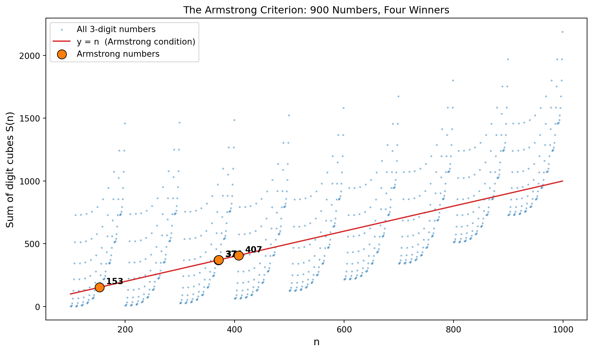

Figure 4.3: For each three-digit number n, the y-axis shows the sum of its digit cubes S(n). The red diagonal is y = n — the Armstrong condition. Only the four points where the cloud touches that line are Armstrong numbers: 153, 370, 371, and 407.

The entire cloud tilts away from the diagonal — most three-digit numbers are far too large or too small for their digit cubes to match them. The four orange dots are the only accidental collisions where the number and its digit-cube sum happen to be equal, making Armstrong numbers genuinely rare treasures.

4.5 Kaprekar’s Process

D._R.Kaprekar was an Indian recreational mathematician who discovered a remarkable fixed-point in 1949 (Kaprekar 1949). Take any four-digit base-10 number that is not a repdigit (all digits the same). Sort its digits from largest to smallest to get a number $A$, and from smallest to largest to get $B$. Compute $A - B$. Repeat. No matter where you start, the process always reaches 6174 in at most seven steps.

# uses: to_base()
def kaprekar_step(n, b=10, ndigits=4):
    s = to_base(n, b).zfill(ndigits)
    desc = int("".join(sorted(s, reverse=True)), b)
    asc  = int("".join(sorted(s)), b)
    return desc - asc

def kaprekar_sequence(n, b=10, ndigits=4):
    seq = [n]
    while True:
        n = kaprekar_step(n, b, ndigits)
        seq.append(n)
        if n == seq[-2]:    # reached fixed point
            break
        if len(seq) > 20:   # safety stop
            break
    return seq

# Test a few starting values
for start in [1234, 5678, 9000, 3087]:
    seq = kaprekar_sequence(start)
    print(f"{start}: {seq}")

1234: [1234, 3087, 8352, 6174, 6174]
5678: [5678, 3087, 8352, 6174, 6174]
9000: [9000, 8991, 8082, 8532, 6174, 6174]
3087: [3087, 8352, 6174, 6174]

6174 is a fixed point: $7641 - 1467 = 6174$. Every four-digit number (with at least two distinct digits) is eventually absorbed into this fixed point.

Does every base have a Kaprekar constant? Not every base and digit length combination works — some lead to cycles rather than a single fixed point.

# uses: to_base(), kaprekar_step()
def find_kaprekar_fixed_points(b, ndigits):
    """Find fixed points of the Kaprekar map in base b."""
    results = set()
    lo = b**(ndigits - 1)      # smallest ndigits number
    hi = b**ndigits            # one past largest
    for n in range(lo, hi):
        s = to_base(n, b).zfill(ndigits)
        if len(set(s)) < 2:    # skip repdigits
            continue
        for _ in range(20):
            n2 = kaprekar_step(n, b, ndigits)
            if n2 == n:
                results.add(n)
                break
            n = n2
    return sorted(results)

print("Base 10, 4 digits:", find_kaprekar_fixed_points(10, 4))
print("Base 10, 3 digits:", find_kaprekar_fixed_points(10, 3))
print("Base 8,  4 digits:", find_kaprekar_fixed_points(8, 4))
print("Base 6,  4 digits:", find_kaprekar_fixed_points(6, 4))

Base 10, 4 digits: [6174]
Base 10, 3 digits: [495]
Base 8,  4 digits: []
Base 6,  4 digits: []

Base 10 with three digits has fixed point 495: $954 - 459 = 495$. Some bases yield empty sets for a given digit length — meaning the process always enters a cycle rather than a fixed point.

Research Example: How Fast Does Every Number Fall Into 6174?

Does every four-digit number converge to 6174 at the same speed, or do some take much longer — and is there a hidden pattern in which numbers take which route?

# uses: kaprekar_step()
import matplotlib.pyplot as plt
import numpy as np

def kap_steps(n, limit=20):
    seen = set()
    k = n
    for i in range(limit):
        if k == 6174:
            return i
        if k in seen or k == 0:
            return limit
        seen.add(k)
        k = kaprekar_step(k)
    return limit

kap_data = np.array([kap_steps(n) for n in range(1000, 10000)])
kap_grid = kap_data.reshape(90, 100)

fig, ax = plt.subplots(figsize=(9, 7.5))
kap_cmap = plt.cm.viridis.copy()
kap_cmap.set_over('white')
im = ax.imshow(kap_grid, aspect='auto', cmap=kap_cmap, vmin=1, vmax=7,
               interpolation='nearest', origin='upper')
cb = fig.colorbar(im, ax=ax, ticks=range(1, 8), extend='max')
cb.set_label('Steps to reach 6174', fontsize=11)
cb.ax.set_yticklabels([str(i) for i in range(1, 8)])
ax.set_xticks([])
ax.set_yticks([])
ax.set_xlabel('1000 to 9999  (left to right, row by row)', fontsize=10)
ax.set_title(
    "Kaprekar's 6174: Every 4-Digit Number by Convergence Speed",
    fontsize=12
)
plt.tight_layout()
plt.show()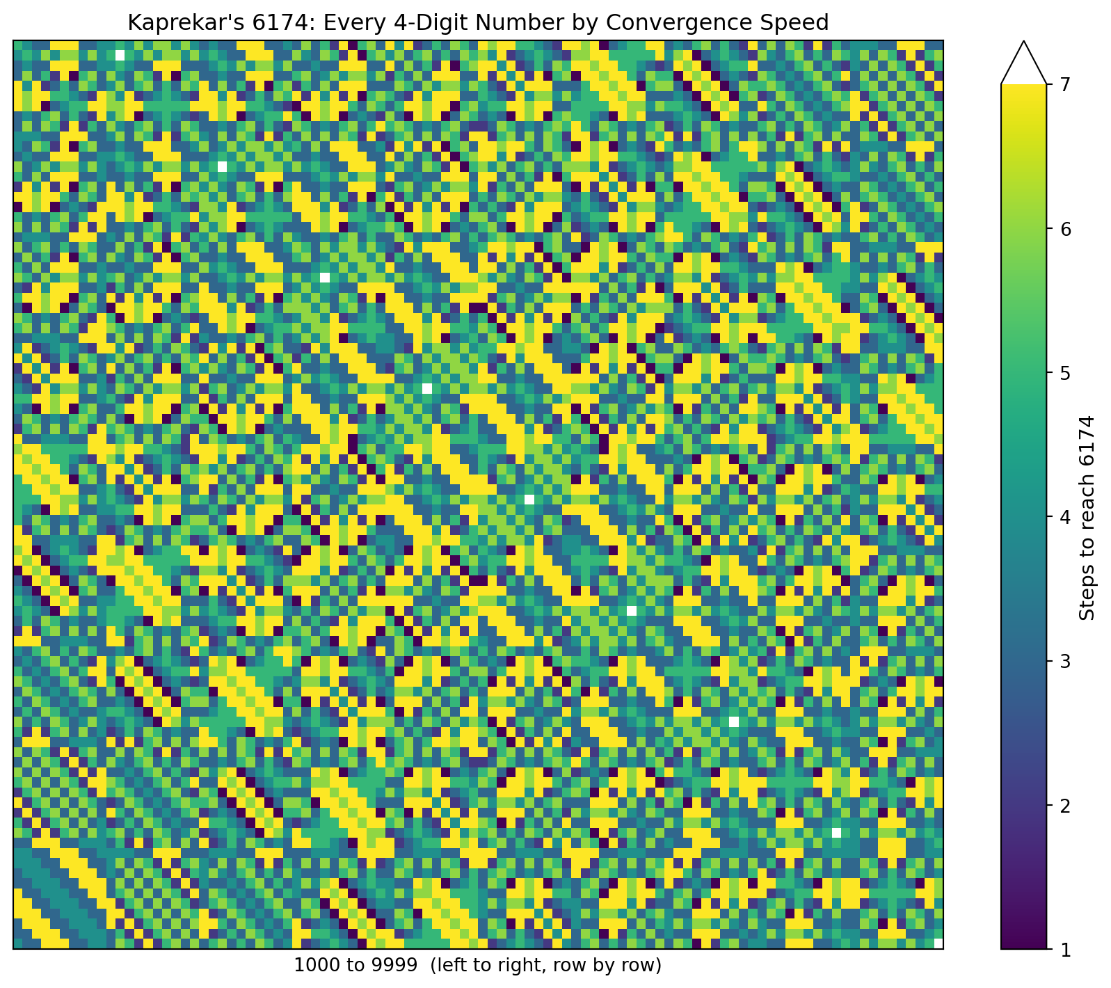

Figure 4.4: All 9000 four-digit numbers (1000–9999) arranged in a 90x100 grid, colored by how many Kaprekar steps each needs to reach 6174. Dark purple = 1 step; bright yellow = 7 steps. White cells are repdigits (1111, 2222, …) — the only four-digit numbers that escape the funnel entirely. The sweeping diagonal bands reveal the hidden pattern: numbers sharing the same set of digits always travel the same path to 6174.

The diagonal bands expose a hidden rule: numbers that share the same four digits (like 1234 and 4321) always land on 6174 in exactly the same number of steps, because sorting them produces identical results. With about fifty lines of Python you just mapped the convergence speed of all 9000 four-digit numbers — that is experimental mathematics.

Numberphile
6174
youtu.be/d8TRcZklX_Q

Demonstrates the Kaprekar constant: subtract any 4-digit number from its reverse-sorted self, repeat, and you always land on 6174 in at most 7 steps.

4.6 Repunit Primes

Marin Mersenne (1588–1648)
French monk and mathematician. His 1644 conjecture about which values of 2^p−1 are prime launched three centuries of prime-hunting. Public domain.

A repunit (short for repeated unit) is a number whose digits are all 1s: $R_n = \underbrace{11 \cdots 1}_{n}$. In base 10, $R_1 = 1$, $R_2 = 11$, $R_3 = 111 = 3 \times 37$, $R_7 = 1111111$. A repunit in base $b$ equals $(b^n - 1)/(b - 1)$.

For $R_n$ to be prime, a necessary condition is that $n$ itself is prime (because $R_{ab} = R_a \cdot Q$ for some integer $Q$). But prime $n$ does not guarantee prime $R_n$ — $R_3 = 111 = 3 \times 37$ has $n = 3$ prime but $R_3$ composite.

from sympy import isprime, factorint
import textwrap

def repunit(n, b=10):
    return (b**n - 1) // (b - 1)

# Which repunits R_n in base 10 are prime for n <= 50?
print("Base-10 repunit primes R_n for n <= 50:")
prime_ns = [
    n for n in range(2, 51)
    if isprime(repunit(n, 10))
]
print(prime_ns)

Base-10 repunit primes R_n for n <= 50:
[2, 19, 23]

In base 10, repunit primes are known for $n = 2, 19, 23, 317, 1031, \ldots$ and are extremely rare. The connection to Chapter 1 (Chapter 1): repunit primes are a special case of the question “what structure must $n$ have for $b^n - 1$ to yield a prime after dividing by $b - 1$?” — the same question that governs Mersenne primes in base 2.

# uses: repunit()
from sympy import isprime

# Mersenne primes are repunit primes in base 2!
# R_n in base 2 = 2^n - 1
print("Base-2 repunit (Mersenne) primes for n <= 40:")
mersenne_ns = [
    n for n in range(2, 41)
    if isprime(repunit(n, 2))
]
print(mersenne_ns)

Base-2 repunit (Mersenne) primes for n <= 40:
[2, 3, 5, 7, 13, 17, 19, 31]

Mersenne primes are exactly the base-2 repunit primes. The study of repunit primes in other bases is an active area of computational number theory where new results are still being found with computers.

4.7 Cyclic Numbers

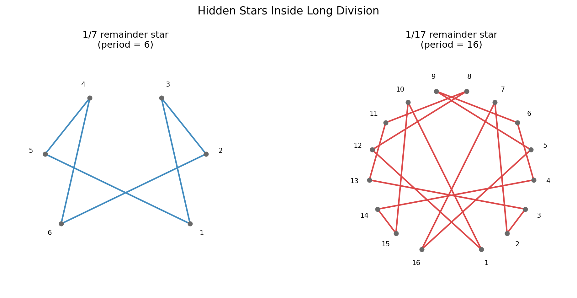
Divide 1 by 7 in long division. The decimal expansion is $0.\overline{142857}$ — a block of six digits that repeats.

from fractions import Fraction
import pprint

def repeating_decimal(p, q, b=10):
    """
    Return the repeating block of p/q in base b.
    Returns (non_repeat_digits, repeat_digits) as lists.
    """
    n = p
    remainders = {}
    digits = []
    pos = 0
    while n != 0:
        if n in remainders:
            start = remainders[n]
            return digits[:start], digits[start:]
        remainders[n] = pos
        n *= b
        digits.append(n // q)
        n %= q
        pos += 1
    return digits, []   # terminating decimal

_, cycle = repeating_decimal(1, 7)
print("Repeating block of 1/7:", cycle)

Repeating block of 1/7: [1, 4, 2, 8, 5, 7]

The block 142857 has a magical property: multiply it by 1, 2, 3, 4, 5, or 6 and you get a cyclic permutation of the same digits.

# uses: repeating_decimal()
block = 142857
for k in range(1, 7):
    product = k * block
    print(f"{k} x {block} = {product}")

1 x 142857 = 142857
2 x 142857 = 285714
3 x 142857 = 428571
4 x 142857 = 571428
5 x 142857 = 714285
6 x 142857 = 857142

$142857 \times 7 = 999999$ — six nines. This is not a coincidence: 7 is a full-reptend prime in base 10. A prime $p$ is full-reptend in base $b$ if the decimal expansion of $1/p$ in base $b$ has a repeating block of length exactly $p - 1$. The length is the multiplicative order of $b$ modulo $p$ (see Section 2.5), so $p$ is full-reptend when that order is as large as possible: $p - 1$.

National Museum of Mathematics
Math Encounters: 142,857
youtu.be/5igZvwEUZNE

Fields Medalist Manjul Bhargava reveals why 142,857 cycles through its own multiples, connecting the repeating decimal of 1/7 to modular arithmetic.

from sympy import n_order, isprime
import math

def is_full_reptend(p, b=10):
    if not isprime(p) or math.gcd(b, p) != 1:
        return False
    return n_order(b, p) == p - 1

# Full-reptend primes in base 10, up to 100
full_reptend = [
    p for p in range(2, 101)
    if is_full_reptend(p)
]
print("Full-reptend primes in base 10 up to 100:")
print(full_reptend)

Full-reptend primes in base 10 up to 100:
[7, 17, 19, 23, 29, 47, 59, 61, 97]

Emil Artin (1898–1962)
Austrian-American algebraist. His 1927 conjecture on primitive roots remains one of the great open problems in number theory. Photo: MFO Archives / CC BY-SA 2.0 DE.

Artin’s conjecture (Artin 1927) — the same conjecture mentioned in Chapter 2 for primitive roots — predicts that there are infinitely many full-reptend primes for any base $b$ that is not a perfect square. The conjecture is still unproved.

Research Example: The Star Hidden Inside Long Division

When you compute 1/7 by long division, the remainders follow a strict sequence before they repeat. If you place those remainders around a circle in order and connect them with lines, what shape do you get — and does the shape change for other full-reptend primes?

# uses: remainder_cycle()
import matplotlib.pyplot as plt
import numpy as np

BLUE = '#1f77b4'
RED  = '#d62728'

def remainder_cycle(p, b=10):
    r, seen, cycle = 1, {}, []
    while r not in seen:
        seen[r] = len(cycle)
        cycle.append(r)
        r = (r * b) % p
    return cycle

def draw_star(ax, p, cycle, color, title):
    theta = {r: 2 * np.pi * r / p - np.pi / 2 for r in range(1, p)}
    for r in range(1, p):
        t = theta[r]
        ax.plot(np.cos(t), np.sin(t), 'o', color='dimgray', ms=5, zorder=5)
        ax.text(1.18 * np.cos(t), 1.18 * np.sin(t), str(r),
                ha='center', va='center', fontsize=8)
    path = cycle + [cycle[0]]
    ax.plot([np.cos(theta[r]) for r in path],
            [np.sin(theta[r]) for r in path],
            color=color, lw=1.8, alpha=0.85)
    ax.set_xlim(-1.45, 1.45)
    ax.set_ylim(-1.45, 1.45)
    ax.set_aspect('equal')
    ax.axis('off')
    ax.set_title(title, fontsize=11)

fig, axes = plt.subplots(1, 2, figsize=(11, 5))
draw_star(axes[0], 7,  remainder_cycle(7),  BLUE,
          '1/7 remainder star\n(period = 6)')
draw_star(axes[1], 17, remainder_cycle(17), RED,
          '1/17 remainder star\n(period = 16)')
fig.suptitle('Hidden Stars Inside Long Division', fontsize=13)
plt.tight_layout()
plt.show()

Figure 4.5: Left: the remainder cycle of 1/7 traces a perfect 6-pointed star on a circle with vertices 1–6. Right: the remainder cycle of 1/17 traces a 16-pointed star visiting all residues 1–16. Both shapes emerge directly from the long-division algorithm — hidden geometry inside ordinary arithmetic.

The star for 1/7 has exactly 6 edges because 7 is a full-reptend prime with period 6 = 7 − 1. The star for 1/17 has 16 edges for the same reason. Every full-reptend prime hides a different star, all of them generated by the same algorithm you learned in fourth grade.

4.8 Base Representation and the Zeckendorf Theorem

Leonardo of Pisa, “Fibonacci” (c. 1170–c. 1250)
Introduced the sequence 1, 1, 2, 3, 5, 8… to Europe in Liber Abaci (1202). The Zeckendorf representation decomposes any integer into a unique sum of non-consecutive Fibonacci numbers. Public domain.

Not every representation requires a fixed base. The Fibonacci base (also called Zeckendorf representation) writes every positive integer as a sum of distinct, non-consecutive Fibonacci numbers.

Zeckendorf’s theorem (Zeckendorf 1972): Every positive integer has a unique such representation. The greedy algorithm works: repeatedly subtract the largest Fibonacci number that fits.

from sympy import fibonacci

def fibonacci_list(up_to):
    fibs = []
    k = 1
    while True:
        f = fibonacci(k)
        if f > up_to:
            break
        fibs.append(f)
        k += 1
    return sorted(fibs, reverse=True)

def zeckendorf(n):
    fibs = fibonacci_list(n)
    terms = []
    for f in fibs:
        if f <= n:
            terms.append(f)
            n -= f
            if n == 0:
                break
    return sorted(terms)

for n in [1, 10, 50, 100, 200]:
    z = zeckendorf(n)
    print(f"{n:3d} = {z}")

  1 = [1]
 10 = [2, 8]
 50 = [3, 13, 34]
100 = [3, 8, 89]
200 = [1, 55, 144]

The Fibonacci base writes each number as a binary-like string of 0s and 1s indexed by Fibonacci numbers, with the constraint that no two adjacent bits are 1. This is the “Fibonacci coding” used in data compression.

# uses: fibonacci_list()
def to_fib_base(n):
    """Return binary string in Fibonacci base (no '11')."""
    fibs = fibonacci_list(n)
    bits = []
    for f in fibs:
        if f <= n:
            bits.append('1')
            n -= f
        else:
            bits.append('0')
    return "".join(bits)

for n in range(1, 16):
    s = to_fib_base(n)
    # verify no two consecutive 1s (Zeckendorf property)
    valid = "11" not in s
    print(f"{n:2d}: {s:10s} valid={valid}")

 1: 10         valid=True
 2: 100        valid=True
 3: 1000       valid=True
 4: 1010       valid=True
 5: 10000      valid=True
 6: 10010      valid=True
 7: 10100      valid=True
 8: 100000     valid=True
 9: 100010     valid=True
10: 100100     valid=True
11: 101000     valid=True
12: 101010     valid=True
13: 1000000    valid=True
14: 1000010    valid=True
15: 1000100    valid=True

Research Example: The Fibonacci Skeleton of Every Integer

Zeckendorf’s theorem guarantees that every positive integer breaks into a unique sum of non-consecutive Fibonacci numbers. What does that decomposition look like across the first 40 integers — and can you see a pattern in which Fibonacci numbers appear most often?

# uses: zeckendorf()
import matplotlib.pyplot as plt
import matplotlib.patches as mpatches
import numpy as np

N = 40
all_fibs  = sorted(set(f for n in range(1, N + 1) for f in zeckendorf(n)))
palette   = plt.cm.viridis(np.linspace(0.1, 0.9, len(all_fibs)))
fib_color = {f: palette[i] for i, f in enumerate(all_fibs)}

fig, ax = plt.subplots(figsize=(14, 5))
for n in range(1, N + 1):
    terms  = sorted(zeckendorf(n))
    bottom = 0
    for f in terms:
        ax.bar(n, f, bottom=bottom, color=fib_color[f],
               edgecolor='white', linewidth=0.4)
        bottom += f

legend_handles = [mpatches.Patch(color=fib_color[f], label=f'F = {f}')
                  for f in all_fibs]
ax.legend(handles=legend_handles, fontsize=8, ncol=4,
          loc='upper left', title='Fibonacci number')
ax.set_xlabel('n', fontsize=12)
ax.set_ylabel('Value (total height = n)', fontsize=12)
ax.set_title(
    'The Fibonacci Skeleton: Every Integer 1–40 Built from Fibonacci Pieces',
    fontsize=12
)
ax.set_xticks(range(1, N + 1))
ax.tick_params(axis='x', labelsize=7)
plt.tight_layout()
plt.show()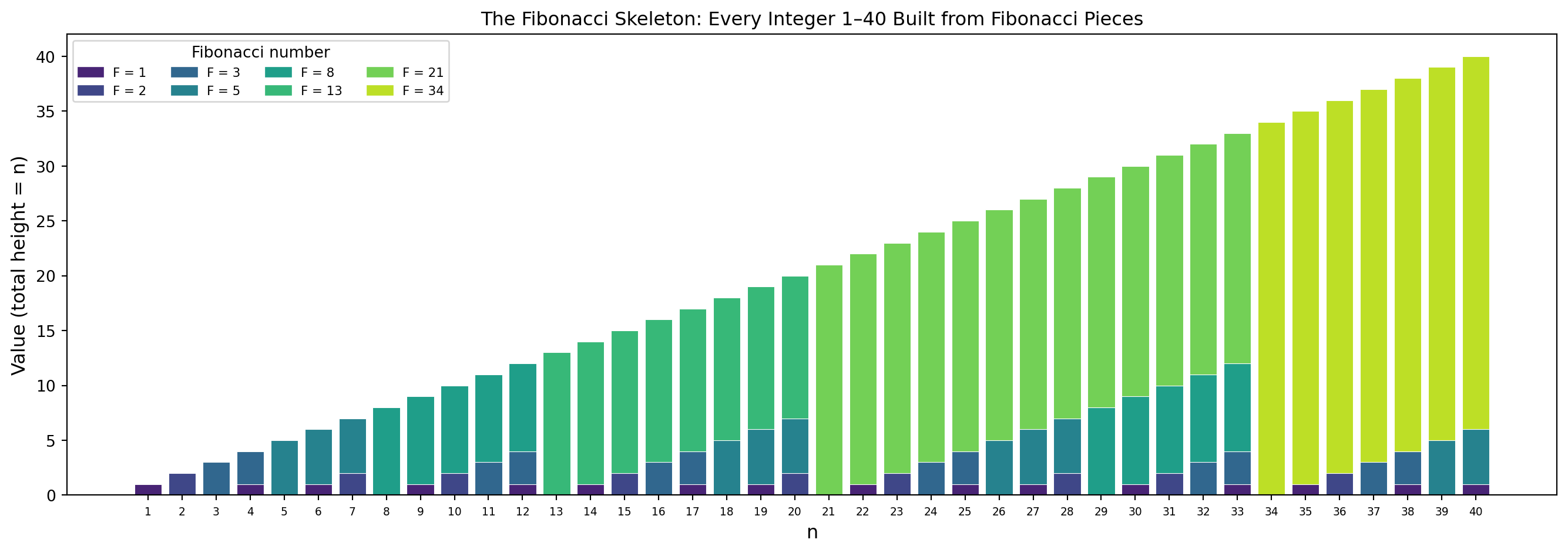

Figure 4.6: Each bar represents an integer from 1 to 40; its height equals that integer, and each colored segment is one Fibonacci number in its Zeckendorf decomposition. Larger Fibonacci numbers (top of the legend) appear in sparser, taller bars, while the small ones (F=1, F=2) fill nearly every bar as gap-fillers.

The bars grow taller exactly as they should — each one is precisely n units high — but the color segments reveal the hidden Fibonacci anatomy inside each integer. Notice how the Fibonacci numbers themselves (1, 2, 3, 5, 8, 13, …) appear as single-color bars, while numbers just below them need the most pieces to fill the gap.

4.9 Further Research Topics

The following topics are arranged from the most accessible to the most open-ended. The first several can be completed in an afternoon; the last few could anchor a semester of independent study.

1. Base conversion by hand. Choose three numbers between 100 and 1000. Convert each to base 2, base 8, and base 16 by performing the repeated-division algorithm by hand, then verify with Python. Reverse-convert the base-2 result back to base 10 by summing powers of 2. Explain why every step in to_base produces digits from right to left (least significant first) even though we print them left to right.