# The Collatz Conjecture: Simple Rules, Deep Mystery {#sec-collatz}
Pick any positive integer. If it is even, divide by 2. If it is odd,
multiply by 3 and add 1. Repeat until you reach 1. That is the entire
rule. You could explain it to a middle-schooler in thirty seconds, yet
as of 2026 no one has proved it always works. Paul Erdős called the
problem "absolutely hopeless" [@lagarias1985], and yet it has a magnetic pull. Computing
reveals its hidden structure far faster than pure thought can. Let us
see what we find.
::: {.content-visible when-format="pdf"}
```{=latex}
\begin{center}
\begin{minipage}[c]{0.28\textwidth}
\centering
\href{https://youtu.be/094y1Z2wpJg}{\includegraphics[width=\textwidth]{images/thumb_094y1Z2wpJg.jpg}}
\end{minipage}%
\hspace{0.02\textwidth}%
\begin{minipage}[c]{0.28\textwidth}
\small\textbf{Veritasium}\\[3pt]
\small The Simplest Math Problem No One Can Solve\\[3pt]
\small\href{https://youtu.be/094y1Z2wpJg}{\texttt{youtu.be/094y1Z2wpJg}}
\end{minipage}%
\hspace{0.02\textwidth}%
\begin{minipage}[c]{0.36\textwidth}
\small Explains the Collatz conjecture, shows the wild trajectories of different starting numbers, and explores why mathematicians believe but cannot prove it always reaches 1.
\end{minipage}
\end{center}
```
:::
::: {.content-visible when-format="html"}
<div style="display:flex; align-items:flex-start; margin:1em 0; gap:12px; width:100%;">
<div style="flex:0 0 200px;"><a href="https://youtu.be/094y1Z2wpJg" target="_blank"><img src="https://img.youtube.com/vi/094y1Z2wpJg/0.jpg" style="width:100%;display:block;" alt="The Simplest Math Problem No One Can Solve"></a></div>
<div style="flex:1; font-size:0.85em;"><strong>Veritasium</strong><br>The Simplest Math Problem No One Can Solve<br><a href="https://youtu.be/094y1Z2wpJg" target="_blank" style="font-family:Consolas,monospace;">youtu.be/094y1Z2wpJg</a></div>
<div style="flex:1; font-size:0.85em;">Explains the Collatz conjecture, shows the wild trajectories of different starting numbers, and explores why mathematicians believe but cannot prove it always reaches 1.</div>
</div>
:::
## A Rule Anyone Can Follow {#sec-collatz-rule}
The **Collatz function** is the map defined by
$$f(n) = \begin{cases}
n / 2 & \text{if } n \text{ is even,} \\
3n + 1 & \text{if } n \text{ is odd.}
\end{cases}$$
Starting from a positive integer $n_0$, we form the **Collatz sequence**
$n_0, f(n_0), f(f(n_0)), \ldots$ and keep applying $f$ until we reach 1.
**Example with $n_0 = 5$.** Since 5 is odd, $f(5) = 16$. Since 16 is
even, $f(16) = 8$. Continuing: $8 \to 4 \to 2 \to 1$. The full
sequence is $\{5, 16, 8, 4, 2, 1\}$, reaching 1 in five steps.
**Example with $n_0 = 6$.** $6 \to 3 \to 10 \to 5 \to 16 \to 8
\to 4 \to 2 \to 1$. Eight steps.
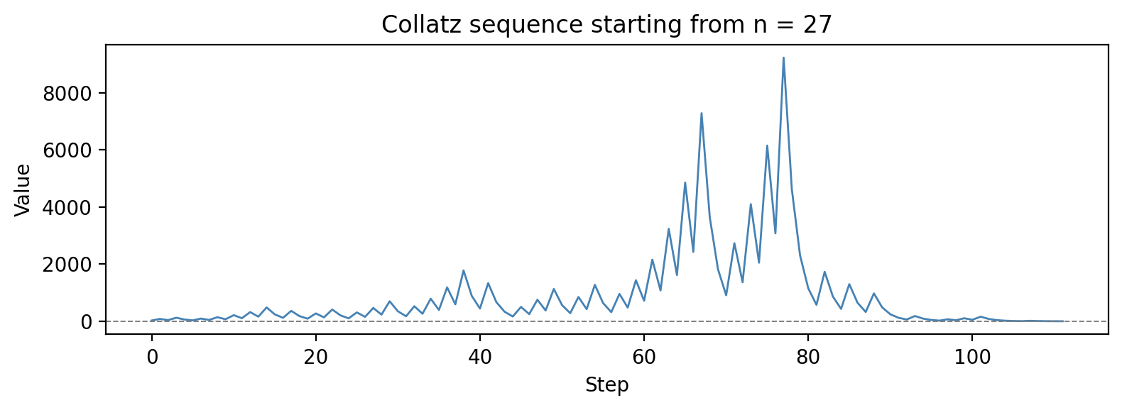
**Example with $n_0 = 27$.** The sequence rises as high as 9232 at
step 77 before finally crashing down to 1 -- after 111 steps. It is
remarkable that a number as small as 27 can produce such a long journey.
The **Collatz conjecture**, first stated by Lothar Collatz in 1937 [@lagarias1985],
claims that for every positive integer $n_0$ the sequence eventually
reaches 1. The conjecture has been verified computationally for every
starting value below $3 \times 10^{20}$ [@barina2021], yet no proof exists.
One family is trivially easy: if $n_0 = 2^k$, the rule halves it $k$
times to reach 1, with no odd steps along the way. Powers of 2 always
terminate, and they terminate quickly. Everything else is a mystery.
## Implementing the Rule as a Loop {#sec-collatz-loop}
The `while` loop introduced in @sec-primes-what is a natural fit: keep
applying the rule while $n \neq 1$, collecting each value. The `%`
operator from @sec-modular-operator tells us whether $n$ is even or odd.
The `//` operator performs **integer (floor) division**, discarding any
remainder: `7 // 2` is 3, not 3.5.
```{python}
def collatz_sequence(n):
    seq = [n]
    while n != 1:
        n = n // 2 if n % 2 == 0 else 3 * n + 1
        seq.append(n)
    return seq

for start in [5, 6, 27]:
    seq = collatz_sequence(start)
    print(f"n={start:3d}: {len(seq)-1:4d} steps, "
          f"max={max(seq):6d}")
```
### Research Example: How Wild Is the Journey From 27 to 1? {.unnumbered .unlisted}
The rule is completely deterministic — every step is forced. Does n = 27 travel quietly to 1, or does it take a spectacular detour first?
```{python}
# uses: collatz_sequence()
import matplotlib.pyplot as plt

seq27 = collatz_sequence(27)
plt.style.use('default')
fig, ax = plt.subplots(figsize=(8, 3))
ax.plot(seq27, lw=1, color='steelblue')
ax.axhline(1, color='gray', lw=0.7, ls='--')
ax.set_xlabel("Step")
ax.set_ylabel("Value")
ax.set_title("Collatz sequence starting from n = 27")
fig.tight_layout()
plt.show()
```
The sequence rockets to 9232 — over 340 times its starting value — at step 77, then crashes to 1 after 111 steps. Every step was forced by the previous one, yet the trajectory looks completely random. You just traced the journey that has captivated mathematicians for 90 years.
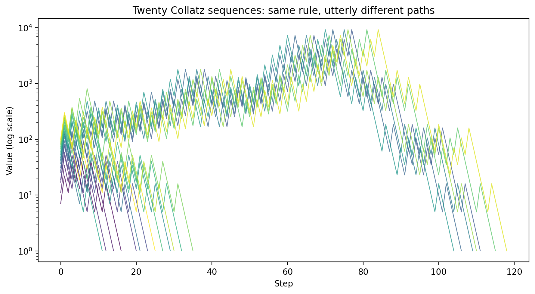
### Research Example: Do All Paths Lead to 1? {.unnumbered .unlisted}
Stack twenty different Collatz trajectories on a single chart — do they all converge, or do some escape upward?
```{python}
#| label: fig-collatz-trajectories
#| fig-cap: "Twenty Collatz sequences overlaid — same rule, twenty utterly different paths, all eventually crashing into 1. Colors run from dark blue (small starts) to bright yellow (larger starts)."
import matplotlib.pyplot as plt

def collatz_sequence(n):
    seq = [n]
    while n != 1:
        n = n // 2 if n % 2 == 0 else 3 * n + 1
        seq.append(n)
    return seq

starts = [7, 11, 17, 19, 25, 27, 31, 37, 41, 43,
          47, 53, 59, 67, 73, 79, 83, 89, 97, 101]
cmap_f = plt.get_cmap('viridis', len(starts))
fig, ax = plt.subplots(figsize=(9, 5))
for i, s in enumerate(starts):
    seq = collatz_sequence(s)
    ax.plot(seq, lw=0.9, alpha=0.75, color=cmap_f(i))
ax.set_xlabel("Step")
ax.set_ylabel("Value (log scale)")
ax.set_yscale('log')
ax.set_title(
    "Twenty Collatz sequences: same rule, utterly different paths"
)
fig.tight_layout()
plt.show()
```
Every thread — no matter how high it climbs or how long it wanders — crashes into 1. Stacking twenty paths turns a conjecture into something you can almost feel. And you produced the whole picture in three lines per trajectory.
## Stopping Times {#sec-collatz-stopping}
The **stopping time** (or **total stopping time**) of $n$ is the number
of steps needed to reach 1: the smallest $k$ such that $f^k(n) = 1$.
```{python}
def stopping_time(n):
    count = 0
    while n != 1:
        n = n // 2 if n % 2 == 0 else 3 * n + 1
        count += 1
    return count

for n in [1, 2, 5, 6, 27]:
    print(f"stopping_time({n:3d}) = {stopping_time(n)}")
```
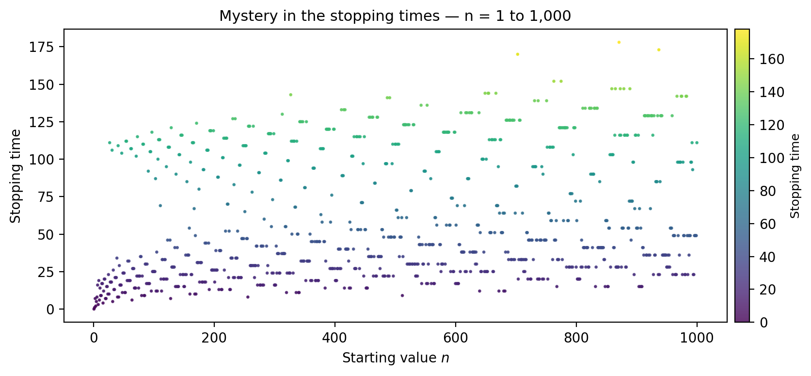
### Research Example: Which Numbers Take the Longest to Reach 1? {.unnumbered .unlisted}
Plot every stopping time from n = 1 to 1,000 — do slow numbers cluster together, or spike up at random with no warning?
```{python}
#| label: fig-collatz-stopping-scatter
#| fig-cap: "Stopping times for n = 1 to 1,000. Most numbers reach 1 in under 100 steps, but isolated spikes — n = 27 being the most dramatic at 111 steps — appear with no pattern."
#| fig-align: center
import matplotlib.pyplot as plt

def stopping_time(n):
    count = 0
    while n != 1:
        n = n // 2 if n % 2 == 0 else 3 * n + 1
        count += 1
    return count

N = 1000
ns = list(range(1, N + 1))
times = [stopping_time(n) for n in ns]
fig, ax = plt.subplots(figsize=(9, 4))
sc = ax.scatter(ns, times, s=2, c=times, cmap='viridis', alpha=0.8)
cb = fig.colorbar(sc, ax=ax, pad=0.01)
cb.set_label('Stopping time', fontsize=9)
ax.set_xlabel("Starting value $n$")
ax.set_ylabel("Stopping time")
ax.set_title(
    "Mystery in the stopping times — n = 1 to 1,000",
    fontsize=11
)
fig.tight_layout()
plt.show()
```
The spike at n = 27 towers over its neighbors at stopping time 111 — more than four times the local average. No formula predicts it. That unpredictability is the Collatz mystery captured in one image, and you produced it in under ten lines.
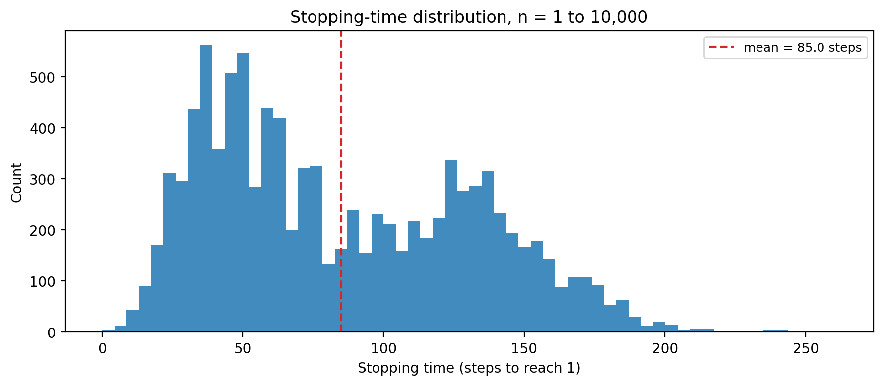
### Research Example: What Does the Full Spread of Journey Lengths Look Like? {.unnumbered .unlisted}
Compute all 10,000 stopping times up to n = 10,000 and plot the distribution — is it symmetric, or skewed with a long tail of stubborn numbers?
```{python}
#| label: fig-collatz-hist
#| fig-cap: "Stopping-time distribution for n = 1 to 10,000 — right-skewed with a heavy tail; the dashed line marks the mean."
import matplotlib.pyplot as plt

BLUE = '#1f77b4'
RED  = '#d62728'

def stopping_time(n):
    count = 0
    while n != 1:
        n = n // 2 if n % 2 == 0 else 3 * n + 1
        count += 1
    return count

all_times = [stopping_time(n) for n in range(1, 10_001)]
mean_t = sum(all_times) / len(all_times)
fig, ax = plt.subplots(figsize=(9, 4))
ax.hist(all_times, bins=60, color=BLUE, edgecolor='none', alpha=0.85)
ax.axvline(mean_t, color=RED, lw=1.5, ls='--',
           label=f'mean = {mean_t:.1f} steps')
ax.set_xlabel('Stopping time (steps to reach 1)')
ax.set_ylabel('Count')
ax.set_title('Stopping-time distribution, n = 1 to 10,000')
ax.legend(fontsize=9)
fig.tight_layout()
plt.show()
```
Most numbers reach 1 in under 150 steps, but a stubborn right tail stretches well past 200 — and that heavy tail is where the mystery hides. You just computed 10,000 stopping times and plotted the full picture in a handful of lines.
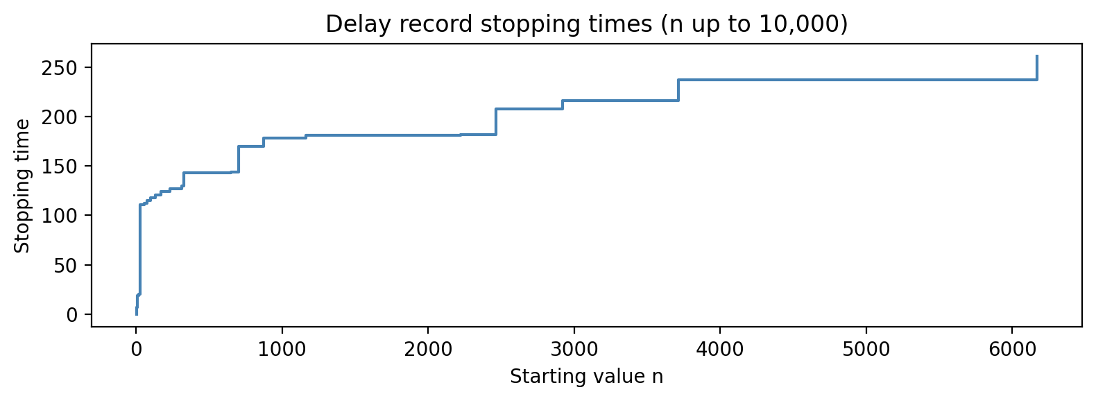
## Delay Records {#sec-collatz-delay}
A **delay record** is a starting value $n$ whose stopping time strictly
exceeds the stopping time of every smaller starting value -- a new
all-time champion for length.
```{python}
# uses: stopping_time()
records = []
best = -1
for n in range(1, 10_001):
    t = stopping_time(n)
    if t > best:
        best = t
        records.append((n, t))

print(f"{'n':>8}  {'stopping time':>14}")
for n, t in records[:20]:
    print(f"{n:8d}  {t:14d}")
```
The delay records grow slowly and irregularly. Notice that $n = 27$
sets a record (111 steps) that is not broken until $n = 54 = 2 \times
27$, which adds exactly one extra halving step at the beginning. Delay
records where $n = 2m$ and $m$ is itself a record are called
**parachute numbers** -- they inherit their length from their half.
### Research Example: How Rare Are Genuine Delay Records? {.unnumbered .unlisted}
How does the record stopping time grow as n increases — in steady stair-steps, or in long flat stretches broken by rare dramatic leaps?
```{python}
import matplotlib.pyplot as plt

def stopping_time(n):
    count = 0
    while n != 1:
        n = n // 2 if n % 2 == 0 else 3 * n + 1
        count += 1
    return count

records = []
best = -1
for n in range(1, 10_001):
    t = stopping_time(n)
    if t > best:
        best = t
        records.append((n, t))

rec_n = [r[0] for r in records]
rec_t = [r[1] for r in records]

fig, ax = plt.subplots(figsize=(8, 3))
ax.step(rec_n, rec_t, where='post',
        color='steelblue', lw=1.5)
ax.set_xlabel("Starting value n")
ax.set_ylabel("Stopping time")
ax.set_title(
    "Delay record stopping times (n up to 10,000)"
)
fig.tight_layout()
plt.show()
```
The staircase has long flat stretches — hundreds of numbers that all fall below the current record — then the bar jumps suddenly when a new champion appears. Records are genuinely rare, and the step function captures that rarity at a glance.
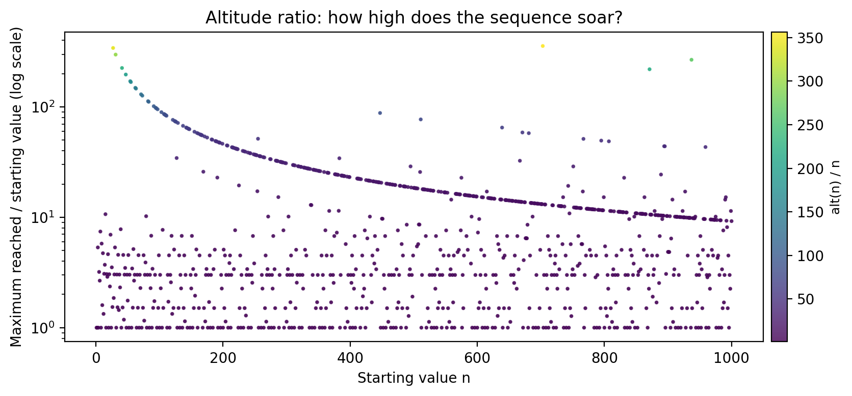
### Research Example: How High Does a Sequence Soar Before Coming Home? {.unnumbered .unlisted}
A related question: how high does a sequence soar before descending? The ratio $\text{alt}(n)/n$ measures it — most numbers barely rise, but a few explode to hundreds of times their starting value.
```{python}
#| label: fig-collatz-altitude
#| fig-cap: "Altitude ratio alt(n)/n for n = 1 to 1,000 — most sequences barely exceed their start, but isolated numbers rocket to 300× their launch value."
import matplotlib.pyplot as plt

def collatz_sequence(n):
    seq = [n]
    while n != 1:
        n = n // 2 if n % 2 == 0 else 3 * n + 1
        seq.append(n)
    return seq

N = 1000
alt_ratios = [max(collatz_sequence(n)) / n for n in range(1, N + 1)]
fig, ax = plt.subplots(figsize=(9, 4))
sc = ax.scatter(range(1, N + 1), alt_ratios, s=3, c=alt_ratios,
                cmap='viridis', alpha=0.8)
cb = fig.colorbar(sc, ax=ax, pad=0.01)
cb.set_label('alt(n) / n', fontsize=9)
ax.set_xlabel('Starting value n')
ax.set_ylabel('Maximum reached / starting value (log scale)')
ax.set_yscale('log')
ax.set_title(
    'Altitude ratio: how high does the sequence soar?'
)
fig.tight_layout()
plt.show()
```
A handful of numbers rocket 300× above their starting value before crashing home — and you found them all in one scatter plot. The rule is always the same; the journey is never predictable.
## The Collatz Graph {#sec-collatz-graph}
Instead of tracing a sequence forward, we can work **backward** from 1:
which numbers flow into 1? Which flow into those? This reverse view
builds the **Collatz tree** [@martin2011].
Under the forward rule, any even number $2m$ maps to $m$. Going
backward: every $m$ has $2m$ as a predecessor. Additionally, any odd
number $q$ satisfying $3q + 1 = n$, meaning $q = (n-1)/3$, is a
predecessor of $n$ -- provided $(n-1)$ is divisible by 3 and $(n-1)/3$
is a positive odd integer.
```{python}
def collatz_preds(n):
    """Return all k with collatz_step(k) == n."""
    result = [2 * n]
    if n > 1 and (n - 1) % 3 == 0:
        m = (n - 1) // 3
        if m >= 1 and m % 2 == 1:
            result.append(m)
    return result

# Who maps to 16?
print("Predecessors of 16:", collatz_preds(16))
for p in collatz_preds(16):
    step = p // 2 if p % 2 == 0 else 3 * p + 1
    print(f"  f({p}) = {step}")
```
We build the backward tree with a **breadth-first search (BFS)**,
expanding predecessors level by level. `collections.deque` is a
double-ended queue that pops from the left in constant time, which
makes BFS efficient.
```{python}
# uses: collatz_preds()
from collections import deque

MAX_DEPTH = 12

children_map = {}
node_level = {1: 0}
level_nodes = {0: [1]}

queue = deque([(1, 0)])
while queue:
    n, d = queue.popleft()
    if d >= MAX_DEPTH:
        continue
    for p in collatz_preds(n):
        if p not in node_level:
            node_level[p] = d + 1
            children_map.setdefault(n, []).append(p)
            level_nodes.setdefault(d + 1, []).append(p)
            queue.append((p, d + 1))

total = sum(len(v) for v in level_nodes.values())
print(f"Total nodes in tree: {total}")
print(f"\n{'depth':>7}  {'nodes':>6}")
for d in range(MAX_DEPTH + 1):
    print(f"{d:7d}  {len(level_nodes[d]):6d}")
```
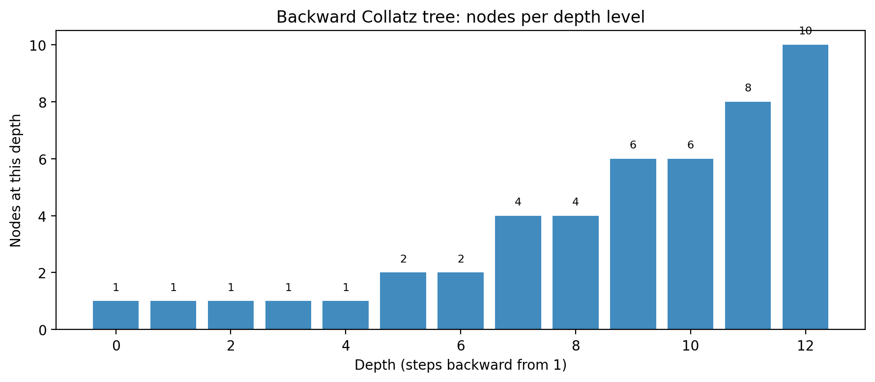
### Research Example: Does the Backward Collatz Tree Branch Fast or Slow? {.unnumbered .unlisted}
The tree fans out as depth grows — each level contains more nodes than the last, hinting at exponential growth. Does the count per level double like a perfect binary tree, or does it grow more slowly?
```{python}
#| label: fig-collatz-tree-growth
#| fig-cap: "Nodes per depth level in the backward Collatz tree rooted at 1. The tree branches roughly by a factor of 1.5 per level — approaching (but never reaching) the factor of 2 implied by the halving rule alone."
from collections import deque
import matplotlib.pyplot as plt

BLUE = '#1f77b4'

def collatz_preds(n):
    result = [2 * n]
    if n > 1 and (n - 1) % 3 == 0:
        m = (n - 1) // 3
        if m >= 1 and m % 2 == 1:
            result.append(m)
    return result

MAX_DEPTH = 12
children_map = {}
node_level = {1: 0}
level_nodes = {0: [1]}
queue = deque([(1, 0)])
while queue:
    n, d = queue.popleft()
    if d >= MAX_DEPTH:
        continue
    for p in collatz_preds(n):
        if p not in node_level:
            node_level[p] = d + 1
            children_map.setdefault(n, []).append(p)
            level_nodes.setdefault(d + 1, []).append(p)
            queue.append((p, d + 1))

depths = list(range(MAX_DEPTH + 1))
counts = [len(level_nodes[d]) for d in depths]
fig, ax = plt.subplots(figsize=(9, 4))
bars = ax.bar(depths, counts, color=BLUE, alpha=0.85)
ax.set_xlabel('Depth (steps backward from 1)')
ax.set_ylabel('Nodes at this depth')
ax.set_title('Backward Collatz tree: nodes per depth level')
for bar, cnt in zip(bars, counts):
    ax.text(bar.get_x() + bar.get_width() / 2, cnt + 0.3, str(cnt),
            ha='center', va='bottom', fontsize=8)
fig.tight_layout()
plt.show()
```
The count grows — but not by a clean factor of 2. Only some nodes gain an odd predecessor; the rest only double. That 1.5× branching rate is a fingerprint of the Collatz rule itself, and you measured it in four lines.
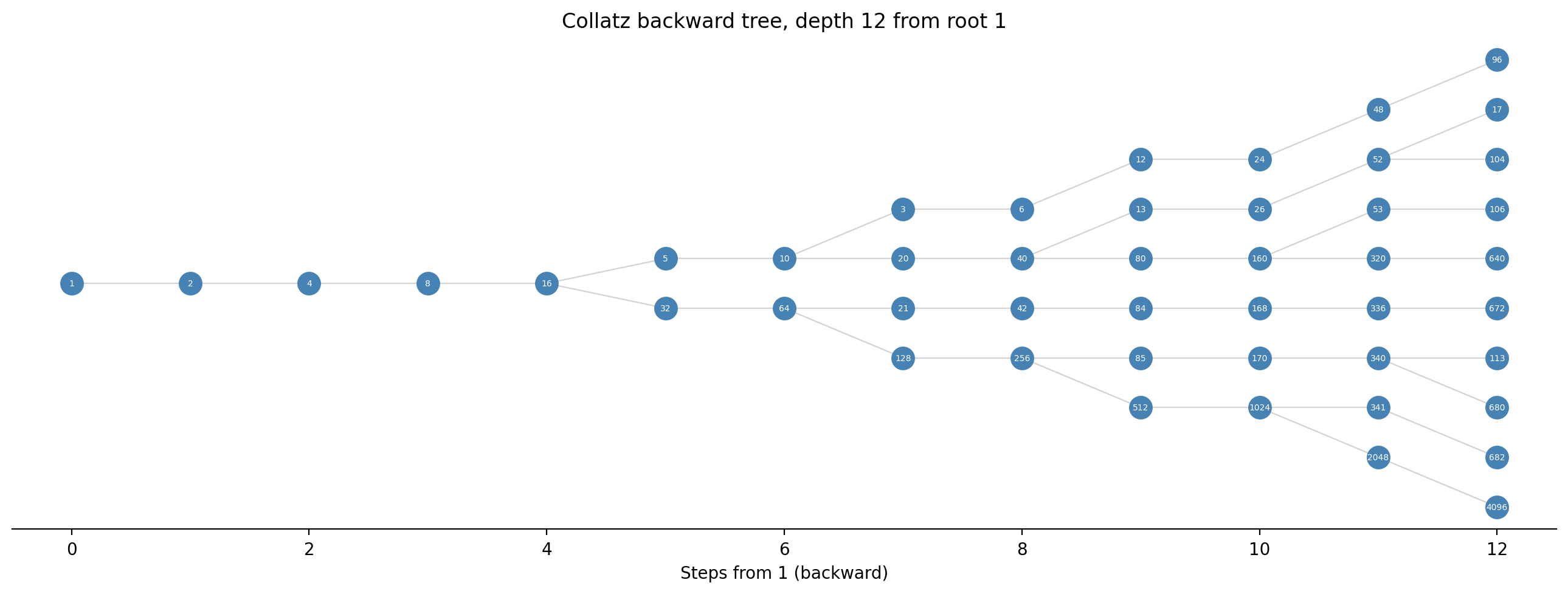
### Research Example: What Does the Collatz Tree Actually Look Like? {.unnumbered .unlisted}
Now we assign positions (depth along $x$, index within level along $y$) and draw the tree — what shape does it take when you can see every branch at once?
```{python}
from collections import deque
import matplotlib.pyplot as plt

def collatz_preds(n):
    result = [2 * n]
    if n > 1 and (n - 1) % 3 == 0:
        m = (n - 1) // 3
        if m >= 1 and m % 2 == 1:
            result.append(m)
    return result

MAX_DEPTH = 12
children_map = {}
node_level = {1: 0}
level_nodes = {0: [1]}
queue = deque([(1, 0)])
while queue:
    n, d = queue.popleft()
    if d >= MAX_DEPTH:
        continue
    for p in collatz_preds(n):
        if p not in node_level:
            node_level[p] = d + 1
            children_map.setdefault(n, []).append(p)
            level_nodes.setdefault(d + 1, []).append(p)
            queue.append((p, d + 1))

pos = {}
for d, group in level_nodes.items():
    w = len(group)
    for i, node in enumerate(group):
        pos[node] = (d, i - (w - 1) / 2.0)

fig, ax = plt.subplots(figsize=(13, 5))
for parent, kids in children_map.items():
    x1, y1 = pos[parent]
    for kid in kids:
        x2, y2 = pos[kid]
        ax.plot([x1, x2], [y1, y2], '-',
                color='lightgray', lw=0.8, zorder=1)
for node, (x, y) in pos.items():
    ax.plot(x, y, 'o', ms=13, color='steelblue',
            zorder=2)
    ax.text(x, y, str(node), ha='center',
            va='center', fontsize=5,
            color='white', zorder=3)
ax.set_xlim(-0.5, MAX_DEPTH + 0.5)
ax.set_xlabel("Steps from 1 (backward)")
ax.set_title(
    "Collatz backward tree, depth 12 from root 1"
)
ax.set_yticks([])
ax.spines['top'].set_visible(False)
ax.spines['right'].set_visible(False)
ax.spines['left'].set_visible(False)
fig.tight_layout()
plt.show()
```
Every branch fans left from 1, and every node carries a specific number — you built this entire picture with a breadth-first search and a handful of `ax.plot` calls. The Collatz conjecture says this tree, extended forever, contains every positive integer exactly once.
Every node in this tree eventually reaches 1 under the Collatz rule. If
the conjecture is true, the complete tree -- extended to infinite depth
with no node-value cutoff -- contains every positive integer exactly
once. The branching pattern you see is real structure, not randomness:
it encodes which numbers have the "bonus" odd predecessor $(n-1)/3$.
## Why Is This So Hard? {#sec-collatz-hard}
```{python}
#| echo: false
from pathlib import Path; import urllib.request
_d = Path('images'); _d.mkdir(exist_ok=True)
_p = _d / 'erdos.jpg'
if not _p.exists():
try: urllib.request.urlretrieve('https://upload.wikimedia.org/wikipedia/commons/2/2f/Erdos_budapest_fall_1992_%28cropped%29.jpg', _p)
except Exception: pass
```
::: {.content-visible when-format="pdf"}
```{=latex}
\begin{center}
\begin{minipage}[c]{0.22\textwidth}
\includegraphics[width=\textwidth]{images/erdos.jpg}
\end{minipage}%
\hspace{0.03\textwidth}%
\begin{minipage}[c]{0.55\textwidth}
\small\textit{Paul Erd\H{o}s (1913--1996)}\\[2pt]
\tiny CC BY 3.0, Kmhkmh, via Wikimedia Commons
\end{minipage}
\end{center}
```
:::
::: {.content-visible when-format="html"}
<div style="display:flex; align-items:center; margin:1em 0; gap:12px;">
<img src="images/erdos.jpg" style="width:100px; flex-shrink:0;" alt="Paul Erdős">
<div style="font-size:0.82em;"><em>Paul Erdős (1913–1996)</em><br><span style="font-size:0.85em;">CC BY 3.0, Kmhkmh, via Wikimedia Commons</span></div>
</div>
:::
The Collatz conjecture has resisted proof for nearly 90 years despite
massive computational evidence. Here is why.
**The heuristic argument.** Whenever $n$ is odd, $3n+1$ is always even
(odd times 3 is odd; odd plus 1 is even). So every odd step is
immediately followed by at least one halving step. Over two steps, an
odd $n$ becomes approximately $3n/2$ -- larger. But $(3n+1)/2$ is often
even again, yielding a second halving: approximately $3n/4$ -- smaller.
The pattern "one tripling, two halvings" multiplies $n$ by
$3 \times \frac{1}{2} \times \frac{1}{2} = \frac{3}{4}$. Since
$3/4 < 1$, this heuristic cycle produces a net decrease.
We can measure this directly. The **geometric mean** of the step ratios
$n_{i+1}/n_i$ tells us the typical factor per step:
```{python}
import math

log_ratios = []
for n in range(2, 501):
    seq = collatz_sequence(n)
    for i in range(len(seq) - 1):
        log_ratios.append(math.log(seq[i + 1] / seq[i]))

geo_mean = math.exp(sum(log_ratios) / len(log_ratios))
print(f"Steps analyzed:       {len(log_ratios)}")
print(f"Geometric mean ratio: {geo_mean:.4f}")
print(f"(below 1 means sequences tend to shrink)")
```
The geometric mean is less than 1, confirming that sequences trend
downward on average. But "on average" is not "always," and that gap is
exactly where the difficulty lives.
**The deep obstacle.** The Collatz rule mixes **multiplication** (the
$3n$ and $/2$ steps) with **addition** (the $+1$). These two worlds
have separate algebraic structures, and their interaction is notoriously
resistant to analysis. A proof would need to show that no number -- not
even one too large to test -- can sustain a sequence that never reaches
1. Numbers that cycle without reaching 1, or that grow without bound,
are theoretically possible but have never been found.
```{python}
#| echo: false
from pathlib import Path; import urllib.request
_d = Path('images'); _d.mkdir(exist_ok=True)
_p = _d / 'tao.jpg'
if not _p.exists():
try: urllib.request.urlretrieve('https://upload.wikimedia.org/wikipedia/commons/d/db/Terence_Tao%2C_PCAST_Member_%28cropped%29.jpg', _p)
except Exception: pass
```
::: {.content-visible when-format="pdf"}
```{=latex}
\begin{center}
\begin{minipage}[c]{0.22\textwidth}
\includegraphics[width=\textwidth]{images/tao.jpg}
\end{minipage}%
\hspace{0.03\textwidth}%
\begin{minipage}[c]{0.55\textwidth}
\small\textit{Terence Tao (b.\ 1975)}\\[2pt]
\tiny Public domain, The White House, via Wikimedia Commons
\end{minipage}
\end{center}
```
:::
::: {.content-visible when-format="html"}
<div style="display:flex; align-items:center; margin:1em 0; gap:12px;">
<img src="images/tao.jpg" style="width:100px; flex-shrink:0;" alt="Terence Tao">
<div style="font-size:0.82em;"><em>Terence Tao (b. 1975)</em><br><span style="font-size:0.85em;">Public domain, The White House, via Wikimedia Commons</span></div>
</div>
:::
**Tao's 2019 result.** In 2019, Terence Tao proved that for "almost
all" starting values (in a precise probabilistic sense covering 100% of
integers), the Collatz sequence eventually drops below any fixed bound
you choose [@tao2022]. This is the strongest rigorous result to date. It stops just
short of the full conjecture -- it does not rule out a single rare
counterexample hiding beyond the reach of any computer.
::: {.content-visible when-format="pdf"}
```{=latex}
\begin{center}
\begin{minipage}[c]{0.28\textwidth}
\centering
\href{https://youtu.be/5mFpVDpKX70}{\includegraphics[width=\textwidth]{images/thumb_5mFpVDpKX70.jpg}}
\end{minipage}%
\hspace{0.02\textwidth}%
\begin{minipage}[c]{0.28\textwidth}
\small\textbf{Numberphile}\\[3pt]
\small UNCRACKABLE? The Collatz Conjecture\\[3pt]
\small\href{https://youtu.be/5mFpVDpKX70}{\texttt{youtu.be/5mFpVDpKX70}}
\end{minipage}%
\hspace{0.02\textwidth}%
\begin{minipage}[c]{0.36\textwidth}
\small A mathematician explains why the Collatz problem has resisted every proof attempt and why even Terence Tao's partial result left the conjecture wide open.
\end{minipage}
\end{center}
```
:::
::: {.content-visible when-format="html"}
<div style="display:flex; align-items:flex-start; margin:1em 0; gap:12px; width:100%;">
<div style="flex:0 0 200px;"><a href="https://youtu.be/5mFpVDpKX70" target="_blank"><img src="https://img.youtube.com/vi/5mFpVDpKX70/0.jpg" style="width:100%;display:block;" alt="UNCRACKABLE? The Collatz Conjecture"></a></div>
<div style="flex:1; font-size:0.85em;"><strong>Numberphile</strong><br>UNCRACKABLE? The Collatz Conjecture<br><a href="https://youtu.be/5mFpVDpKX70" target="_blank" style="font-family:Consolas,monospace;">youtu.be/5mFpVDpKX70</a></div>
<div style="flex:1; font-size:0.85em;">A mathematician explains why the Collatz problem has resisted every proof attempt and why even Terence Tao's partial result left the conjecture wide open.</div>
</div>
:::
```{python}
#| echo: false
from pathlib import Path; import urllib.request
_d = Path('images'); _d.mkdir(exist_ok=True)
_p = _d / 'Alan_Turing_(1951)_(crop).jpg'
if not _p.exists():
try: urllib.request.urlretrieve('https://upload.wikimedia.org/wikipedia/commons/6/66/Alan_Turing_%281951%29_%28crop%29.jpg', _p)
except Exception: pass
```
::: {.content-visible when-format="pdf"}
```{=latex}
\begin{center}
\begin{minipage}[c]{0.22\textwidth}
\includegraphics[width=\textwidth]{images/Alan_Turing_(1951)_(crop).jpg}
\end{minipage}%
\hspace{0.03\textwidth}%
\begin{minipage}[c]{0.55\textwidth}
\small\textit{Alan Turing (1912--1954)}\\[2pt]
\tiny Public domain, Elliott \& Fry, via Wikimedia Commons
\end{minipage}
\end{center}
```
:::
::: {.content-visible when-format="html"}
<div style="display:flex; align-items:center; margin:1em 0; gap:12px;">
<img src="images/Alan_Turing_(1951)_(crop).jpg" style="width:100px; flex-shrink:0;" alt="Alan Turing">
<div style="font-size:0.82em;"><em>Alan Turing (1912–1954)</em><br><span style="font-size:0.85em;">Public domain, Elliott & Fry, via Wikimedia Commons</span></div>
</div>
:::
**The halting problem parallel.** Turing showed in 1936 [@turing1936] that no
algorithm can decide, in general, whether an arbitrary computer program
will ever stop running. The Collatz rule is one specific program, not an
arbitrary one, so Turing's theorem does not directly apply. But the
comparison is instructive: a rule that iterates in an unpredictable,
pseudo-random way resembles a general computation, and that is precisely
why it resists the kind of clean inductive arguments that work for most
problems in number theory.
## Further Research Topics {#sec-collatz-research}
The following topics are listed in order of increasing difficulty.
Start by exploring computationally, form a conjecture from what you
observe, then try to explain it.
**1. Powers of 2.**
Compute `stopping_time(2**k)` for $k = 1, 2, \ldots, 20$. Observe that
the answer is always $k$. Write a proof by induction: if $n = 2^k$,
then every step is a halving (the odd rule never fires), so after exactly
$k$ halvings we reach $2^0 = 1$.
*(Adapted from @martin2011.)*
**3. Even vs. odd starting values.**
Compute the average stopping time separately for even and odd starting
values below 10000. Which group takes longer on average? Notice that
every even $n = 2m$ satisfies $\text{stopping\_time}(2m) =
\text{stopping\_time}(m) + 1$. Use this to explain the difference
between the two distributions without computing a single stopping time
from scratch.
*(Problem proposed by Claude Code.)*
**4. How fast does the maximum grow?**
For $N = 100, 200, 400, \ldots, 10000$, record the largest stopping time
found for starting values up to $N$. Plot maximum stopping time vs.
$\log N$. Does the maximum appear to grow roughly linearly with $\log N$?
If so, estimate the proportionality constant and state a precise
conjecture.
*(Problem proposed by Claude Code.)*
**5. Delay record characterization.**
Extend the delay record search to $n = 1, \ldots, 1{,}000{,}000$.
For each delay record holder, check whether it is odd or even. Among the
odd delay record holders, examine their prime factorizations. Do they
share any small prime factors (2, 3, 5, ...)? Do records tend to occur
in clusters near powers of 2? State a conjecture based on your
observations.
*(Problem proposed by Claude Code.)*
**6. Parachute numbers.**
Call $n$ a **parachute number** if $n = 2m$ where $m$ is itself a delay
record holder. Parachute numbers inherit stopping time $= \text{stopping\_time}(m) + 1$
for free. Remove all parachute numbers from the list of delay records.
What is left? Are the remaining "genuine" records odd or even? Can you
find a pattern among them?
*(Problem proposed by Claude Code.)*
**7. The Syracuse shortcut.**
Define $T(n) = (3n+1)/2$ for odd $n$ and $T(n) = n/2$ for even $n$.
This collapses every odd step plus its guaranteed first even step into a
single operation. Compare the stopping time under $T$ to
$\text{stopping\_time}(n)$ for $n = 1, \ldots, 1000$. What is the exact
algebraic relationship between the two counts? Can you prove it?
*(Problem proposed by Claude Code.)*
**8. Parity sequences.**
For a Collatz sequence, record the parity at each step: `'E'` (even) or
`'O'` (odd). For $n = 5$, the sequence $5, 16, 8, 4, 2, 1$ gives the
parity string `OEEEE`. For $n = 1, \ldots, 200$, collect all distinct
parity strings. How many distinct strings are there? Can two different
starting values produce the exact same parity string? Is there a starting
value with parity string `OEO`? What is the shortest parity string that
uniquely identifies a starting value?
*(Problem proposed by Claude Code.)*
**9. The inverse tree without depth limits.**
The code in @sec-collatz-graph built the backward tree to depth 12.
Remove the depth limit and instead stop when no new nodes can be added
without exceeding 10000. For each depth level $d = 0, 1, \ldots$, count
the number of nodes in the tree at that depth. Does the count grow
faster than linearly? Faster than exponentially? Compare this growth
rate to powers of 2.
*(Problem proposed by Claude Code.)*
**10. Collatz sequences in binary.**
In binary, dividing an even number by 2 is simply dropping the last
digit (a right shift). Write the Collatz rule for an odd binary number
$n$ by working out what $3n + 1$ does to the last three bits of $n$.
For example, if the last three bits of $n$ are `001` (meaning $n \equiv
1 \pmod{8}$), compute the last three bits of $3n+1$. Make a table for
all odd patterns of the last 3 bits. Do starting values sharing the same
last $k$ binary digits always diverge after a fixed number of steps?
*(Problem proposed by Claude Code.)*
**11. Number of odd steps.**
Let $\text{odd}(n)$ be the number of odd-valued terms in the Collatz
sequence of $n$ (not counting the final 1). Compute $\text{odd}(n)$ for
$n = 1, \ldots, 1000$. Plot $\text{odd}(n)$ vs. $\text{stopping\_time}(n)$.
Conjecture a formula: what fraction of all steps are odd steps, on
average? Hint: use the observation that $3n+1$ is always even to bound
the ratio.
*(Problem proposed by Claude Code.)*
**12. Generalized Collatz: the $qn+1$ problem.**
Replace $3n+1$ with $5n+1$ (keeping the even rule $n/2$). Test all
starting values from 1 to 1000. Does every sequence reach 1? If not,
find the smallest starting value that does not converge to 1 and
describe what happens to that sequence instead. Repeat for $7n+1$ and
$9n+1$. Formulate a conjecture about which values of $q$ lead to
universal convergence.
*(Adapted from @martin2011.)*
**13. Collatz and arithmetic progressions.**
Fix a modulus $m$. For each residue class $r \in \{0, 1, \ldots, m-1\}$,
compute the average stopping time of all $n \leq 10000$ with
$n \equiv r \pmod m$. Try $m = 3, 4, 6$, and 8. Which residue classes
consistently produce the longest stopping times? Explain any patterns
you find using the structure of the Collatz rule modulo $m$ -- for
instance, what does the rule do to all numbers congruent to 1 mod 4
in one step?
*(Problem proposed by Claude Code.)*
**14. Statistical self-similarity.**
The stopping-time scatter plot for $n = 1, \ldots, N$ looks visually
similar whether $N = 100$ or $N = 10000$. To test this, compute the
stopping-time histogram for $N = 500, 1000, 2000, 5000$, normalizing
each histogram so that the bin heights sum to 1 and the horizontal axis
runs from 0 to 1 (divide each stopping time by the maximum stopping time
for that $N$). Do the normalized histograms converge to the same shape
as $N$ grows? This type of shape-preservation under rescaling is called
**self-similarity** and is a defining feature of the fractals we will
study in Chapter 12.
*(Problem proposed by Claude Code.)*
**15. Proving a small special case.**
Prove that every number of the form $n = 4k + 2$ (i.e., $n \equiv 2
\pmod 4$) reaches a smaller value within exactly two steps:
$n \to n/2 \to n/4$. Then prove that every $n \equiv 0 \pmod 4$ reaches
a smaller value in at most two steps. More ambitiously, characterize
all $n$ for which the sequence is guaranteed to decrease within three
steps. Try to chain such guarantees: use a three-step decrease guarantee
to prove a six-step decrease guarantee for a larger class of numbers.
This "bootstrapping" approach is the closest anyone has come to a
direct structural proof.
*(Problem proposed by Claude Code.)*
**17. Stopping time vs. total stopping time.**
The *stopping time* of $n$ is the number of steps until the sequence
first falls strictly below $n$. The *total stopping time* is the
number of steps until the sequence reaches 1. These can differ
dramatically: $n = 97$ has stopping time 3 (the sequence drops below
97 after just three steps) yet total stopping time 118. Compute both
quantities for all $n = 1, \ldots, 10000$ and plot the gap
$\text{total\_stopping\_time}(n) - \text{stopping\_time}(n)$. What is
the average gap? Does the gap correlate with the altitude ratio
$\text{alt}(n)/n$ you computed in the previous project? Find the
starting value below 10000 with the largest gap. Explain intuitively
why a number can fall quickly from its starting value yet still wander
for a long time before reaching 1.
*(Problem proposed by Claude Code.)*
**18. Negative integers.**
The Collatz rule makes perfect sense for negative integers: if $n$ is
even, replace $n$ by $n/2$; if $n$ is odd, replace $n$ by $3n + 1$.
Apply this rule to all starting values $n = -1, -2, \ldots, -200$.
You will discover that instead of converging to 1, negative integers
fall into *cycles* — the conjecture is actually false over the
negatives! Find all distinct cycles that appear. There are exactly
three: a 2-cycle starting at $-1$, a 5-cycle starting at $-5$, and an
18-cycle starting at $-17$ [@lagarias1985]. Verify each cycle by hand for the
2-element case. For starting values below $-200$, do any new cycles
appear, or does every negative integer eventually land in one of these
three? Write a program that, given a starting value, identifies which
cycle it enters and after how many steps. Use your findings to explain
why proving the Collatz conjecture for *positive* integers is so much
harder than it might appear: positive integers have only one known
attractor, but nothing in the rule itself forbids additional cycles.
*(Problem proposed by Claude Code.)*
**19. Gaussian integers.**
A *Gaussian integer* is a complex number $a + bi$ where $a$ and $b$
are integers. Define a Collatz-like map on Gaussian integers: if $a$
and $b$ are both even, apply $n \mapsto n/2$; if $a + b$ is odd
(exactly one of $a, b$ is odd), apply $n \mapsto 3n + 1$; if $a + b$
is even but not both zero, apply $n \mapsto n/2$. Explore what
happens for all Gaussian integers $a + bi$ with $|a|, |b| \leq 10$.
Do the sequences converge? If not, do they enter cycles? Can you find
a Gaussian integer whose sequence grows without bound? This is an
open research area: the behavior of Collatz-like maps over $\mathbb{Z}[i]$
is not fully understood [@martin2011, p. 755].
*(Adapted from @martin2011.)*
**20. Two-variable Collatz.**
Design your own two-dimensional Collatz-like map on pairs of positive
integers $(m, n)$. One natural choice: if both $m$ and $n$ are even,
apply $(m, n) \to (m/2, n/2)$; if $m$ is odd, apply $(m, n) \to
(3m + 1, n)$; if $n$ is odd (and $m$ is even), apply $(m, n) \to
(m, 3n + 1)$. Write a program to iterate your map from all starting
pairs with $1 \leq m, n \leq 50$. Do all pairs eventually reach
$(1, 1)$? If not, what other attractors exist? Adjust your rules and
explore whether different choices lead to more or fewer cycles. Once
you have explored computationally, formulate a precise conjecture about
your map and attempt to prove even the simplest special case, such as
pairs of the form $(2^j, 2^k)$ [@martin2011, p. 756].
*(Adapted from @martin2011.)*


_(crop).jpg)