# Computational Misleads: When Computers Lie {#sec-misleads}
## The Danger of Computational Evidence {#sec-misleads-danger}
> "The purpose of computing is insight, not numbers."
> --- R. W. Hamming
A computer reveals patterns that would take centuries to find by hand.
But a tool that powerful can also mislead.
This chapter collects cautionary tales from experimental mathematics:
cases where computation strongly suggested a false pattern, where
standard arithmetic silently discarded significant digits, and where a
result looked unmistakably like something it was not.
The safeguard is not to distrust computers -- it is to understand how
they work.
### A Famous Near-Miss
Suppose you ask a computer to evaluate $e^{\pi\sqrt{163}}$ and round
the answer to the nearest integer.
With only 15 significant decimal digits, standard floating-point
arithmetic cannot reliably compute even the last few digits of the
integer part of a number near $2.6 \times 10^{17}$.
We need `mpmath` (introduced at @sec-constants-mpmath) to look more
carefully:
```{python}
import mpmath       # see @sec-constants-mpmath
import textwrap

mpmath.mp.dps = 50
val  = mpmath.exp(mpmath.pi * mpmath.sqrt(163))
n    = int(val)    # floor: largest integer <= val
frac = val - n
print(f"Floor:   {n}")
s = mpmath.nstr(frac, 18)
# width=60 wraps long output to fit the printed page
print("Excess:")
print(textwrap.fill(s, width=60))
```
The excess above the floor is $0.999999999999250\ldots$ -- exactly
twelve nines before the first non-nine digit.
If a calculation cuts off after 12 decimal places and rounds, it
sees $0.999999999999 \approx 1$ and concludes the number equals the
integer $262{,}537{,}412{,}640{,}768{,}744$.
That conclusion is wrong.
The number is transcendental -- not an integer -- but a thirteenth
decimal place is needed to expose the deception.
The number 163 is one of the nine so-called Heegner numbers, which
arise in the theory of complex multiplication.
That theory explains why $e^{\pi\sqrt{163}}$ is so extraordinarily
close to an integer.
Our point here is simpler: twelve zeros (or nines) in a row prove
nothing by themselves [@borwein2009crucible, Ch. 10].
## Patterns That Fail Eventually {#sec-misleads-fail}
### Euler's Prime-Generating Formula
Leonhard Euler noticed in 1772 that the formula $n^2 + n + 41$
produces a prime for $n = 0, 1, 2, \ldots, 39$ [@hardywright1979].
Forty consecutive primes is a striking pattern:
```{python}
from sympy import isprime   # see @sec-primes-what

run = 0
for n in range(100):
    if isprime(n*n + n + 41):
        run += 1
    else:
        print(f"Prime for n = 0 to {n-1} ({run} values)")
        print(f"Fails at n={n}: {n*n+n+41} = {n+1}^2")
        break
```
At $n = 40$ the formula gives $40^2 + 40 + 41 = 1681 = 41^2$,
obviously composite.
No polynomial with integer coefficients can produce only primes: if
$p(n)$ is prime for all $n$, then $p(n + p(0))$ is divisible by
$p(0)$ for every $n$, eventually producing a composite value.
The 40-case streak is a remarkable coincidence, not a theorem.
### Fermat Numbers
Pierre de Fermat conjectured in 1650 that every number of the form
$F_k = 2^{2^k} + 1$ is prime [@hardywright1979].
The first five cooperate beautifully:
```{python}
from sympy import factorint   # see @sec-primes-what

for k in range(6):
    fk = 2**(2**k) + 1
    fs = factorint(fk)
    if len(fs) == 1:
        print(f"F_{k} = {fk:>11}  prime")
    else:
        parts = " * ".join(
            f"{p}^{e}" if e > 1 else str(p)
            for p, e in sorted(fs.items())
        )
        print(f"F_{k} = {fk:>11}  = {parts}")
```
Euler showed in 1732 that $F_5 = 641 \times 6{,}700{,}417$ [@hardywright1979], nearly
a century after Fermat's conjecture.
Today no Fermat prime beyond $F_4$ is known, and several $F_k$
for $k > 4$ have been completely factored.
Five confirming cases were not enough.
### The 11,056 Surprise
Some patterns hold for far more than forty cases before breaking [@borwein2009crucible, Ch. 10].
Define the sequence
$$u_{n+2} = \left\lfloor 1 + \frac{u_{n+1}^2}{u_n} \right\rfloor,
\quad u_0 = 8,\; u_1 = 55.$$
```{python}
import pprint

def u_next(prev, curr):
    return 1 + curr * curr // prev

u = [8, 55]
for _ in range(10):
    u.append(u_next(u[-2], u[-1]))

# width=60 wraps long output to fit the printed page
pprint.pprint(u, width=60, compact=True)
```
These values match the Taylor coefficients of the rational function
$$R(x) = \frac{8 + 7x - 7x^2 - 7x^3}{1 - 6x - 7x^2 + 5x^3 + 6x^4}$$
for every $n$ up to $10{,}000$ -- and then the match breaks for the
very first time at $n = 11{,}056$.
Ten thousand confirming cases and still wrong.
Two more famous conjectures followed the same script.
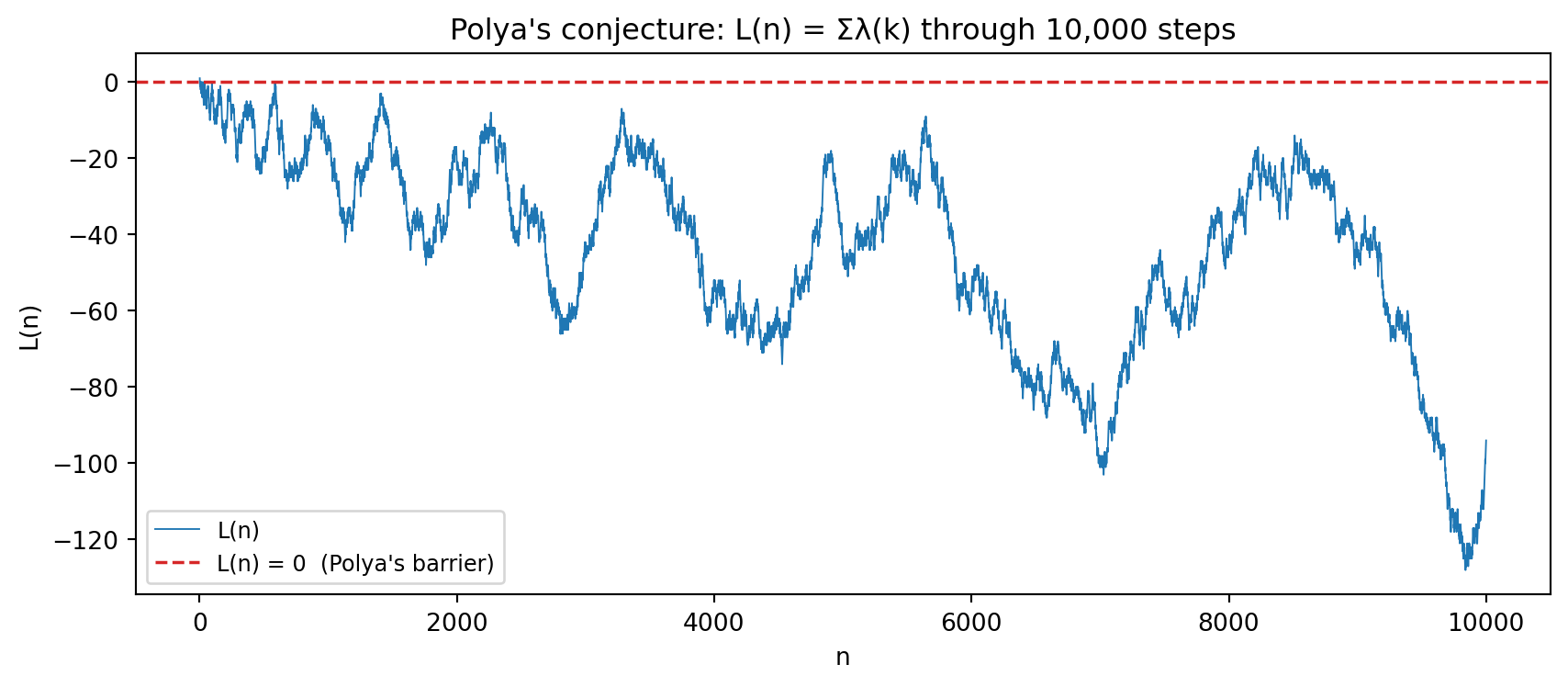
Pólya conjectured in 1919 [@polya1919] that the running sum
$L(n) = \sum_{k=1}^n \lambda(k) \le 0$ for all $n \ge 2$,
where $\lambda(n) = (-1)^{\Omega(n)}$ and $\Omega(n)$ counts prime
factors with multiplicity.
Watch $L(n)$ through ten thousand steps:
### Research Example: Does the Liouville Sum Ever Cross Zero? {.unnumbered .unlisted}
Pólya's conjecture says $L(n) \le 0$ for every $n \ge 2$ — that numbers with an
odd count of prime factors are always at least as plentiful as those with an even
count. Does the graph through 10,000 terms give any reason to doubt this?
```{python}
#| label: fig-misleads-polya
#| fig-cap: "Polya's conjecture: L(n) = Σλ(k) stays at or below zero for n = 1 to 10,000. Haselgrove proved in 1958 that the conjecture eventually fails — but you would never guess it from this graph."
import matplotlib.pyplot as plt

BLUE = '#1f77b4'
RED  = '#d62728'

N_pol = 10_000
lam_pol = [0] * (N_pol + 1)
lam_pol[1] = 1
is_prime_pol = [True] * (N_pol + 1)
primes_pol = []
for i in range(2, N_pol + 1):
    if is_prime_pol[i]:
        primes_pol.append(i)
        lam_pol[i] = -1
    for p in primes_pol:
        if i * p > N_pol:
            break
        is_prime_pol[i * p] = False
        lam_pol[i * p] = -lam_pol[i]
        if i % p == 0:
            break

L_pol = []
s_pol = 0
for n in range(1, N_pol + 1):
    s_pol += lam_pol[n]
    L_pol.append(s_pol)

fig, ax = plt.subplots(figsize=(9, 4))
ax.plot(range(1, N_pol + 1), L_pol, lw=0.7, color=BLUE, label='L(n)')
ax.axhline(0, color=RED, lw=1.3, ls='--', label='L(n) = 0  (Polya\'s barrier)')
ax.set_xlabel('n')
ax.set_ylabel('L(n)')
ax.set_title("Polya's conjecture: L(n) = Σλ(k) through 10,000 steps")
ax.legend(fontsize=9)
fig.tight_layout()
plt.show()
```
The curve never leaves negative territory throughout all 10,000 steps — the conjecture
looks rock-solid. Yet Haselgrove proved in 1958 [@haselgrove1958] that $L(n)$ must eventually cross zero,
and the smallest known counterexample lies near $n = 906{,}000{,}000$: invisible at any
scale we can easily plot.
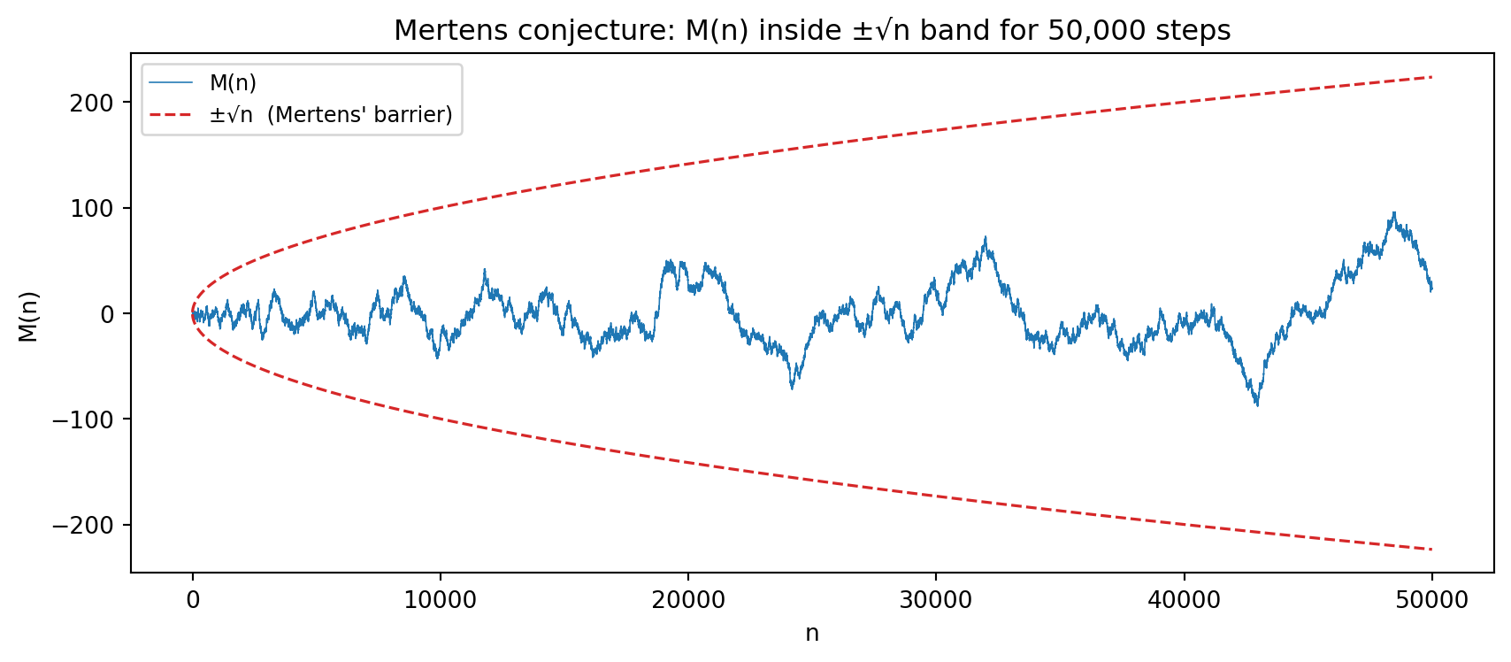
The Mertens conjecture ran even longer.
The Mertens function $M(n) = \sum_{k=1}^n \mu(k)$, where $\mu(k)$
is the Möbius function, was conjectured by Mertens in 1897 [@mertens1897] to satisfy
$|M(n)| < \sqrt{n}$ for all $n \ge 1$.
Odlyzko and te Riele disproved it in 1985 [@odlyzkoterie1985] — but the smallest explicit
counterexample has still never been found.
Fifty thousand steps give no hint of trouble:
### Research Example: Does the Mertens Function Ever Escape Its Band? {.unnumbered .unlisted}
The Mertens conjecture claims $M(n)$ stays strictly inside the $\pm\sqrt{n}$ corridor
for every $n$. Plot both the function and the barrier for 50,000 steps and decide
whether the evidence looks overwhelming — or whether the graph is simply too short.
```{python}
#| label: fig-misleads-mertens
#| fig-cap: "Mertens conjecture: M(n) stays well inside the ±√n band for all 50,000 steps shown. The conjecture was disproved in 1985, yet no explicit counterexample has ever been exhibited."
import numpy as np
import matplotlib.pyplot as plt

BLUE = '#1f77b4'
RED  = '#d62728'

N_mer = 50_000
mu_mer = [0] * (N_mer + 1)
mu_mer[1] = 1
is_prime_mer = [True] * (N_mer + 1)
primes_mer = []
for i in range(2, N_mer + 1):
    if is_prime_mer[i]:
        primes_mer.append(i)
        mu_mer[i] = -1
    for p in primes_mer:
        if i * p > N_mer:
            break
        is_prime_mer[i * p] = False
        if i % p == 0:
            mu_mer[i * p] = 0
            break
        else:
            mu_mer[i * p] = -mu_mer[i]

M_mer = []
m_mer = 0
for n in range(1, N_mer + 1):
    m_mer += mu_mer[n]
    M_mer.append(m_mer)

ns_mer = np.arange(1, N_mer + 1)
sqrt_n = np.sqrt(ns_mer)

fig, ax = plt.subplots(figsize=(9, 4))
ax.plot(ns_mer, M_mer, lw=0.6, color=BLUE, label='M(n)')
ax.plot(ns_mer,  sqrt_n, lw=1.2, ls='--', color=RED, label='±√n  (Mertens\' barrier)')
ax.plot(ns_mer, -sqrt_n, lw=1.2, ls='--', color=RED)
ax.set_xlabel('n')
ax.set_ylabel('M(n)')
ax.set_title("Mertens conjecture: M(n) inside ±√n band for 50,000 steps")
ax.legend(fontsize=9)
fig.tight_layout()
plt.show()
```
The Mertens function hugs the center and never comes close to the red boundary — every
data point screams "true!" Yet the conjecture is false, disproved not by a clever
calculation but by the indirect machinery of the Riemann zeta function: the
counterexample lives somewhere beyond $10^{30}$, utterly beyond reach of any plot.
::: {.content-visible when-format="pdf"}
```{=latex}
\begin{center}
\begin{minipage}[c]{0.28\textwidth}
\centering
\href{https://youtu.be/pQs_wx8eoQ8}{\includegraphics[width=\textwidth]{images/thumb_pQs_wx8eoQ8.jpg}}
\end{minipage}%
\hspace{0.02\textwidth}%
\begin{minipage}[c]{0.28\textwidth}
\small\textbf{PBS Infinite Series}\\[3pt]
\small Why Computers are Bad at Algebra\\[3pt]
\small\href{https://youtu.be/pQs_wx8eoQ8}{\texttt{youtu.be/pQs\_wx8eoQ8}}
\end{minipage}%
\hspace{0.02\textwidth}%
\begin{minipage}[c]{0.36\textwidth}
\small Floating-point arithmetic gives every number a tiny rounding error --- and those errors compound, cancel catastrophically, and silently invalidate results that look perfectly reasonable.
\end{minipage}
\end{center}
```
:::
::: {.content-visible when-format="html"}
<div style="display:flex; align-items:flex-start; margin:1em 0; gap:12px; width:100%;">
<div style="flex:0 0 200px;"><a href="https://youtu.be/pQs_wx8eoQ8" target="_blank"><img src="https://img.youtube.com/vi/pQs_wx8eoQ8/0.jpg" style="width:100%;display:block;" alt="Why Computers are Bad at Algebra"></a></div>
<div style="flex:1; font-size:0.85em;"><strong>PBS Infinite Series</strong><br>Why Computers are Bad at Algebra<br><a href="https://youtu.be/pQs_wx8eoQ8" target="_blank" style="font-family:monospace;">youtu.be/pQs_wx8eoQ8</a></div>
<div style="flex:1; font-size:0.85em;">Floating-point arithmetic gives every number a tiny rounding error — and those errors compound, cancel catastrophically, and silently invalidate results that look perfectly reasonable.</div>
</div>
:::
## Floating-Point Arithmetic {#sec-misleads-float}
Every number you compute in standard Python is stored as a
64-bit *double-precision float* following the IEEE 754 standard.
This gives about 15 to 16 significant decimal digits.
That limit is usually invisible -- until it isn't.
### The 0.1 + 0.2 Problem
```{python}
a = 0.1
b = 0.2
c = a + b

print(c == 0.3)          # Is it exactly 0.3?
print(f"{c:.17f}")       # Show 17 decimal places
print(f"{0.3:.17f}")     # True 0.3 for comparison
```
The number $0.1$ cannot be represented exactly in binary
floating-point, just as $1/3$ cannot be represented exactly in
decimal.
The nearest 64-bit float is slightly more than $0.1$, and adding
two such approximations accumulates the error.
This is not a bug -- it is how binary arithmetic works.
### Machine Epsilon
*Machine epsilon* is the smallest positive number $\varepsilon$ such
that $1 + \varepsilon \neq 1$ in floating-point arithmetic.
We can discover it experimentally:
```{python}
import math

eps = 1.0
while 1.0 + eps != 1.0:
    eps /= 2.0
eps *= 2.0      # last eps that still changes 1.0 + eps
print(f"Machine epsilon: {eps:.3e}")
print(f"Significant digits: ~{-math.log10(eps):.1f}")
```
Machine epsilon for 64-bit doubles is approximately
$2.22 \times 10^{-16}$, corresponding to about 15.7 significant
decimal digits.
Any result that depends on digits beyond the 15th must be verified
by a different method.
For the $e^{\pi\sqrt{163}}$ calculation, we need dozens of digits --
far beyond what standard floats can provide.
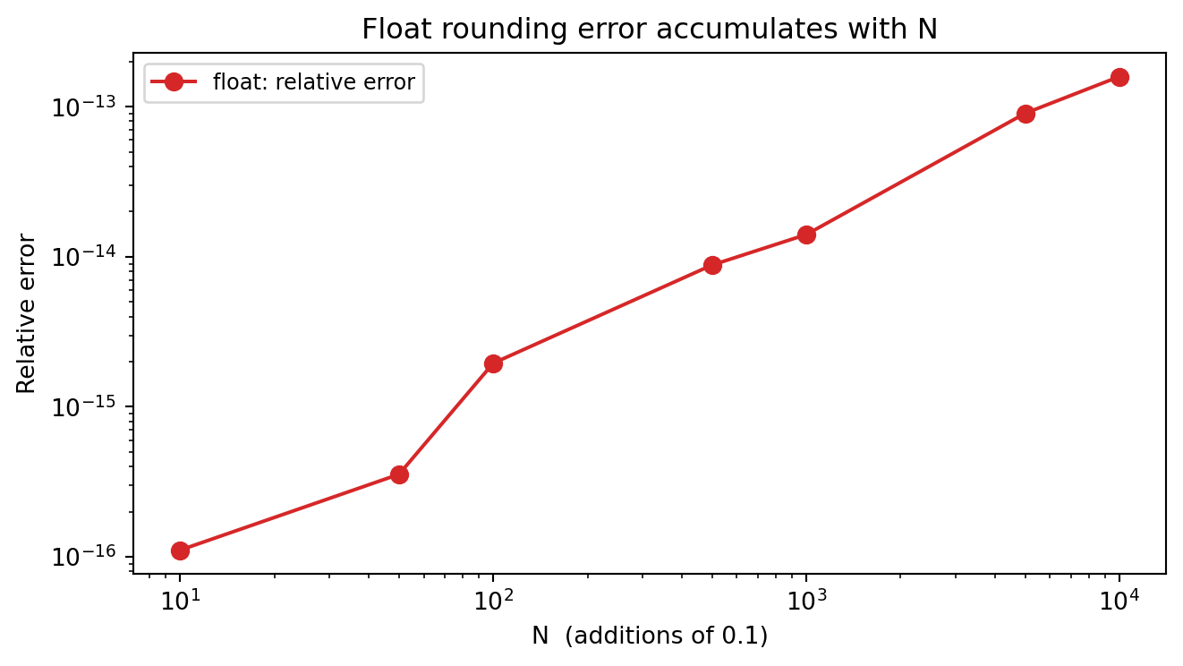
The error does not stay constant — it accumulates.
Every time you add `0.1` to a running total, you carry a tiny rounding
residual forward.
After $N$ additions the residual is of order $N \times \varepsilon$:
### Research Example: Does Repeated Addition Accumulate Error? {.unnumbered .unlisted}
Each time Python adds `0.1` to a running total, a tiny rounding residual tags along.
Add `0.1` exactly $N$ times and compare the result to the exact value $N/10$ — does
the error stay flat, or does it grow with $N$?
```{python}
#| label: fig-misleads-floaterr
#| fig-cap: "Relative error when summing 0.1 exactly N times using Python float. The error grows with N. With Fraction(1, 10) the error stays exactly zero throughout."
import matplotlib.pyplot as plt

RED = '#d62728'

Ns = [10, 50, 100, 500, 1_000, 5_000, 10_000]
errs = []
for N in Ns:
    total = 0.0
    for _ in range(N):
        total += 0.1
    errs.append(abs(total - N / 10) / (N / 10))

fig, ax = plt.subplots(figsize=(7, 4))
ax.loglog(Ns, errs, 'o-', color=RED, lw=1.5, ms=7,
          label='float: relative error')
ax.set_xlabel('N  (additions of 0.1)')
ax.set_ylabel('Relative error')
ax.set_title('Float rounding error accumulates with N')
ax.legend(fontsize=9)
fig.tight_layout()
plt.show()
```
The log-log plot traces a straight line — the error grows roughly proportionally to $N$.
Add `0.1` ten times and the mistake is invisible; add it ten thousand times and the
relative error has climbed by a factor of a thousand, silently corrupting any result that
depends on the final digit.
## Exact Arithmetic as Safeguard {#sec-misleads-exact}
Python provides three tools for exact or high-precision arithmetic
that sidestep float rounding entirely.
**Integer arithmetic** is always exact in Python.
Integers can be arbitrarily large and every operation is precise.
**`fractions.Fraction`** (introduced at @sec-cfrac-convergents)
stores rationals as exact integer pairs:
```{python}
from fractions import Fraction  # see @sec-cfrac-convergents

a = Fraction(1, 10)    # exact 1/10
b = Fraction(2, 10)    # exact 2/10
total = a + b
print(total)                      # 3/10
print(total == Fraction(3, 10))   # True
```
**SymPy** (introduced at @sec-primes-what) works with symbolic
expressions and can evaluate sums and products exactly.
**`mpmath`** (introduced at @sec-constants-mpmath) allows arbitrary
decimal precision for transcendental computations, as demonstrated in
@sec-misleads-danger.
The right tool depends on the problem:
| Answer type | Tool |
|-------------|------|
| Exact rational | `int`, `Fraction` |
| Closed symbolic form | SymPy |
| Irrational to many decimals | `mpmath` |
| Exploratory estimate | `float` |
Use standard `float` for exploration but confirm critical results
with one of the exact tools above.
## Catastrophic Cancellation {#sec-misleads-cancellation}
*Catastrophic cancellation* occurs when two nearly equal numbers are
subtracted: the leading digits cancel and the remaining digits are
dominated by rounding noise.
### A Clear Example
Consider $\sqrt{x+1} - \sqrt{x}$ for large $x$.
Both square roots are close to $\sqrt{x}$, so their difference is
tiny, but the subtraction throws away most of the significant digits:
```{python}
import math

def diff_naive(x):
    return math.sqrt(x + 1) - math.sqrt(x)

def diff_stable(x):
    # Multiply and divide by the conjugate (sqrt(x+1)+sqrt(x))
    # to get the algebraically equivalent 1/(sqrt(x+1)+sqrt(x))
    return 1.0 / (math.sqrt(x + 1) + math.sqrt(x))

for exp in [4, 8, 12, 16]:
    x  = 10.0**exp
    nv = diff_naive(x)
    sv = diff_stable(x)
    print(f"x=1e{exp:02d}: naive={nv:.4e}  stable={sv:.4e}")
```
At $x = 10^{16}$ the naive result is exactly $0$ -- all significant
digits have cancelled.
The stable formula computes the same mathematical value by rewriting
it as $1/(\sqrt{x+1} + \sqrt{x})$, which involves no dangerous
subtraction.
### The Quadratic Formula
The same trap appears in the quadratic formula for $x^2 + bx + c = 0$:
$$x = \frac{-b \pm \sqrt{b^2 - 4c}}{2}.$$
When $|b|$ is large and $|c|$ is small, one root suffers catastrophic
cancellation.
The stable fix uses *Vieta's formula*: if $r_1 \cdot r_2 = c$,
compute the large root accurately first, then recover the small root
as $r_2 = c / r_1$.
```{python}
import math

def roots_naive(b, c):
    d = math.sqrt(b*b - 4.0*c)
    return (-b + d) / 2.0, (-b - d) / 2.0

def roots_stable(b, c):
    d = math.sqrt(b*b - 4.0*c)
    # Compute the large root with no cancellation
    r1 = (-b - d) / 2.0 if b > 0 else (-b + d) / 2.0
    r2 = c / r1          # Vieta: r1 * r2 = c
    return r1, r2

b, c = 1e8, 1.0
_, rn2 = roots_naive(b, c)
_, rs2 = roots_stable(b, c)
print(f"Naive  small root: {rn2:.6e}")
print(f"Stable small root: {rs2:.6e}")
print(f"True   small root: {c/(-b):.6e}")
```
The naive formula loses all significant digits for the small root;
the stable formula recovers it exactly.
## The Strong Law of Small Numbers {#sec-misleads-small-numbers}
```{python}
#| echo: false
from pathlib import Path; import urllib.request
_d = Path('images'); _d.mkdir(exist_ok=True)
_p = _d / 'guy.jpg'
if not _p.exists():
try: urllib.request.urlretrieve('https://upload.wikimedia.org/wikipedia/commons/5/5a/Richard_K_Guy_2005.jpg', _p)
except Exception: pass
```
::: {.content-visible when-format="pdf"}
```{=latex}
\begin{center}
\begin{minipage}[c]{0.22\textwidth}
\includegraphics[width=\textwidth]{images/guy.jpg}
\end{minipage}%
\hspace{0.03\textwidth}%
\begin{minipage}[c]{0.55\textwidth}
\small\textit{Richard K. Guy (1916--2020)}\\[2pt]
\tiny CC BY 2.0, Thane Plambeck, via Wikimedia Commons
\end{minipage}
\end{center}
```
:::
::: {.content-visible when-format="html"}
<div style="display:flex; align-items:center; margin:1em 0; gap:12px;">
<img src="images/guy.jpg" style="width:100px; flex-shrink:0;" alt="Richard K. Guy">
<div style="font-size:0.82em;"><em>Richard K. Guy (1916–2020)</em><br><span style="font-size:0.85em;">CC BY 2.0, Thane Plambeck, via Wikimedia Commons</span></div>
</div>
:::
Mathematician Richard Guy formalized a principle that experienced
researchers recognize instinctively [@guy1988]:
> "There aren't enough small numbers to meet the many demands made
> of them."
Small numbers have so many special properties that coincidental
patterns are almost inevitable.
A pattern that holds for $n = 1, 2, \ldots, 10$ is weak evidence.
Forty consecutive cases (Euler's formula) or ten thousand consecutive
cases (the $u_n$ sequence) are stronger -- but as we have seen,
still not proof.
### The Circle-Chord Example
Draw $n$ points on a circle, connect every pair with a chord, and
count the maximum number of regions the interior is divided into.
The first five values look unmistakable:
```{python}
import math   # math.comb introduced at @sec-pascal-binomial

def circle_regions(n):
    # Exact formula: C(n,4) + C(n,2) + 1
    return math.comb(n, 4) + math.comb(n, 2) + 1

print(f"{'n':>2}  {'regions':>7}  {'2^(n-1)':>7}")
for n in range(1, 9):
    r = circle_regions(n)
    p = 2**(n - 1)
    note = "" if r == p else "  <-- FAILS"
    print(f"{n:>2}  {r:>7}  {p:>7}{note}")
```
For $n = 1$ through $5$ the answer is $1, 2, 4, 8, 16$ -- perfect
powers of two.
Almost every student who sees this table writes down the conjecture
$2^{n-1}$.
At $n = 6$ the true formula gives $\binom{6}{4} + \binom{6}{2} + 1
= 15 + 15 + 1 = 31$, not $32$.
The correct formula counts distinct chord intersections inside the
circle; it is $\binom{n}{4} + \binom{n}{2} + 1$, which has nothing
to do with powers of two.
The first five values are a coincidence.
### Why This Matters
Every pattern in this chapter -- Euler's formula, Fermat numbers,
the circle-chord count -- appeared convincing from small cases.
Computation found the patterns, and computation also revealed where
they break.
The lesson is not that computation is untrustworthy.
It is that computation is a source of *hypotheses*, not *theorems*.
The next step after finding a pattern is always to search for a proof
or to push the computation far enough to look for a counterexample.
You will see how to turn a computational observation into a properly
documented conjecture in Chapter 15.
## Further Research Topics {#sec-misleads-research}
1. Verify that the formula $n^2 + n + 41$ gives a prime for
$n = 0$ to $39$ and fails at $n = 40$.
Why does it fail at $n = 40$ specifically?
Hint: substitute $n = 41 - 1$ and factor.
Does the formula fail again at $n = 41$?
*(Problem proposed by Claude Code.)*
2. Find the "prime streak" length for the formulas $n^2 + n + 17$
and $n^2 + n + 5$ by testing each $n$ from 0 upward until the
formula produces a composite.
Write a Python function `prime_streak(k)` that returns the
length of the streak for the formula $n^2 + n + k$.
Which values of $k$ up to 100 give the longest streaks?
*(Problem proposed by Claude Code.)*
3. Confirm that $F_5 = 2^{32} + 1$ is divisible by 641 using only
modular arithmetic: compute `pow(2, 32, 641)` and explain what
the result means.
Then find the smallest prime factor of $F_6 = 2^{64} + 1$ using
`sympy.factorint`.
*(Problem proposed by Claude Code.)*
4. The machine epsilon loop doubles `eps` at the end to undo the
final halving.
Rewrite the loop to find epsilon without that final correction.
Now try replacing `float` with `fractions.Fraction` throughout
the loop.
What happens and why?
*(Problem proposed by Claude Code.)*
5. The circle-chord formula $\binom{n}{4} + \binom{n}{2} + 1$ counts
regions by counting the number of intersection points inside the
circle.
Draw the diagram for $n = 4$ and $n = 5$, count the intersections
by hand, and verify that the formula matches.
For $n = 6$, two chords can intersect at the same interior point
if three or more points are collinear -- how does this affect the
count?
*(Problem proposed by Claude Code.)*
6. Implement the $u_n$ sequence (Section 2) and compute 200 terms.
Plot the values on a log scale.
Fit a line to $\log(u_n)$ vs. $n$ to estimate the growth rate.
Does $u_n$ grow exponentially?
*(Problem proposed by Claude Code.)*
7. Catastrophic cancellation in alternating series: compute the
alternating harmonic series $1 - 1/2 + 1/3 - 1/4 + \cdots$ up
to $N = 100{,}000$ terms using `float` and using
`fractions.Fraction`.
The true sum is $\ln 2 \approx 0.6931471805599453$.
How large is the relative error in the float version?
Which summation order (left to right vs. smallest terms first)
reduces float error?
*(Problem proposed by Claude Code.)*
8. The Heegner numbers are
$d = 1, 2, 3, 7, 11, 19, 43, 67, 163$ [@borwein2009crucible].
For each $d$, use `mpmath` at 60 decimal places to compute
$e^{\pi\sqrt{d}}$ and find how many consecutive 9s (or 0s)
appear in its decimal expansion after the integer part.
Which Heegner numbers produce the most dramatic near-integers?
Why might $d = 163$ be so much more extreme than $d = 43$?
*(Problem proposed by Claude Code.)*
9. *Sinc integrals* [@borwein2009crucible]:
The product integrals
$I_k = \int_0^\infty \frac{\sin x}{x} \cdot \frac{\sin(x/3)}{x/3}
\cdots \frac{\sin(x/(2k-1))}{x/(2k-1)}\, dx$
equal $\pi/2$ for $k = 1, 2, \ldots, 7$ but $I_8 \ne \pi/2$
(the deviation is roughly $10^{-10}$).
Use `scipy.integrate.quad` to evaluate $I_1$, $I_2$, $I_3$
numerically and confirm they equal $\pi/2$ to the limit of
numerical accuracy.
Then attempt $I_8$ and see whether the deviation is visible.
*(Problem proposed by Claude Code.)*
10. A *Carmichael number* [@carmichael1910] passes Fermat's primality test (see
@sec-modular-fermat) for every base $a$ coprime to it, yet it is
composite.
The smallest is $561 = 3 \times 11 \times 17$.
Use Python to find all Carmichael numbers up to $10{,}000$ by
checking whether $n$ is composite but $a^{n-1} \equiv 1 \pmod n$
for all $a$ with $\gcd(a, n) = 1$.
How many are there?
This is another example of a pattern (Fermat's test passing)
that misleads the computationalist.
*(Problem proposed by Claude Code.)*
11. *Benford's law check* [@benford1938]: Benford's law predicts that the leading
digit $d$ of numbers drawn from many natural data sets appears
with frequency $\log_{10}(1 + 1/d)$.
Use `mpmath` to compute the first 10{,}000 terms of the sequence
$2^n$ and record each term's leading digit.
Do the frequencies match Benford's law?
Repeat for $3^n$, $n!$, and the Fibonacci numbers.
Which sequences obey Benford's law and which do not?
Can you explain the difference?
*(Problem proposed by Claude Code.)*
12. *Experimental vs. proof*:
Choose any pattern in this chapter that failed -- Euler's
formula, Fermat numbers, or the circle-chord count.
Write a complete mathematical proof that the pattern must
eventually fail, documenting it in the style described in
Chapter 15: state a precise conjecture, show the computational
evidence that motivated it, give the proof, and explain what
makes the proof more convincing than any finite number of
examples.
Why can no computation alone ever replace a proof?
*(Problem proposed by Claude Code.)*
13. *Near-integer coincidences among $e$ and $\pi$* [@borwein2009crucible]:
Use `mpmath` at 30 decimal places to evaluate $e^\pi - \pi$,
$\pi^e$, $e^{1/\pi}$, and $\pi^{1/e}$.
Which is closest to an integer?
Now conduct a systematic search: for integer exponents
$a, b \in \{-3, -2, -1, 0, 1, 2, 3\}$ compute $e^a \pi^b$
and record the ten combinations closest to whole numbers.
Do any match coincidences already catalogued in the
mathematical literature?
(Hint: $e^\pi - \pi \approx 19.9991$.)
Explain why such near-misses are expected by probabilistic
reasoning rather than deep number-theoretic structure.
*(Problem proposed by Claude Code.)*
14. *Euler's trinomial--Fibonacci coincidence*:
The trinomial number $t_n$ is the coefficient of $x^0$ in
$(x + 1 + x^{-1})^n$, equivalently the middle coefficient
of $(1 + x + x^2)^n$.
Use `sympy.Poly` to expand $(1 + x + x^2)^n$ and extract
the middle coefficient for $n = 0, 1, \ldots, 15$.
Let $F_n$ denote the Fibonacci numbers.
Verify that $3t_{n+1} - t_{n+2} = F_n(F_n + 1)$ holds for
$n = 0, 1, \ldots, 7$ but fails at $n = 8$.
Plot the difference $3t_{n+1} - t_{n+2} - F_n(F_n+1)$ for
$n = 0, \ldots, 15$ to show how quickly the pattern
collapses.
Why is a seven-case coincidence far more seductive — and
more dangerous — than a three-case one?
*(Problem proposed by Claude Code.)*
15. *The 268-digit near-integer*:
Define
$$S = 81 \sum_{n=1}^{\infty} \frac{\lfloor n \tanh \pi \rfloor}{10^n}.$$
Using `mpmath` at 50, then 100, then 320 decimal places,
compute partial sums out to $N = 400$ terms and report how
many decimal places of $S$ agree with $1$.
Explain analytically why the agreement persists for exactly
268 digits: because $\tanh\pi \approx 0.99627$, the floor
$\lfloor n \tanh\pi \rfloor = n - 1$ for all $n \le 268$,
turning the sum into $81\sum (n-1)/10^n = 1$ exactly; only
at $n = 269$ does the floor first drop to $n - 2$,
introducing a tiny error.
At what precision does `mpmath` first reveal that $S \ne 1$?
(This is one of the most spectacular near-integers in
experimental mathematics. [@borwein2009crucible, Ch. 10])
*(Adapted from @borwein2009crucible.)*
16. *Giuga's conjecture* [@giuga1950]:
Every prime $p$ satisfies
$1^{p-1} + 2^{p-1} + \cdots + (p-1)^{p-1} \equiv -1 \pmod p$
by Fermat's little theorem.
Giuga conjectured in 1950 that the converse is also true:
only primes satisfy this congruence.
Use `pow(k, n-1, n)` (Python's built-in modular
exponentiation) to test all integers $n$ from $4$ to
$10{,}000$.
Do any composites pass?
A *Giuga number* is a composite $n$ where every prime factor
$p$ of $n$ satisfies $p \mid (n/p - 1)$.
Verify that Giuga numbers are exactly the composites that
would refute the conjecture.
The smallest known Giuga number has six prime factors and
is $30 = 2 \cdot 3 \cdot 5$ — wait, does $30$ pass the
congruence test?
How does Giuga's conjecture compare to the Korselt
criterion that characterises Carmichael numbers from
Topic 10?
*(Problem proposed by Claude Code.)*
17. *The 40-digit cosine product*:
Define
$$I_K = \int_0^\infty \cos(2x)\prod_{k=1}^{K} \cos\!\left(\frac{x}{k}\right) dx.$$
For small $K$ this integral equals $\pi/8$ exactly.
Using `mpmath.quad` at 60 decimal places (not `scipy`),
compute $I_K$ for $K = 5, 10, 20, 50$ and compare each
result to `mpmath.pi / 8`.
```python
import mpmath
mpmath.mp.dps = 60

def cosine_integrand(x, K):
    prod = mpmath.cos(2 * x)
    for k in range(1, K + 1):
        prod *= mpmath.cos(x / k)
    return prod

for K in [5, 10, 20, 50]:
    val = mpmath.quad(lambda x: cosine_integrand(x, K),
                      [0, mpmath.inf])
    diff = val - mpmath.pi / 8
    print(f"K={K:2d}  I_K - π/8 = {diff:.6e}")
```
At what value of $K$ does $I_K$ first measurably differ from
$\pi/8$ at 60-digit precision?
The difference is astronomically small — smaller than
$10^{-40}$ for moderate $K$ — yet provably nonzero for
sufficiently large $K$ [@borwein2009crucible, Ch. 10].
Explain in your own words why 40 digits of agreement is
*not* evidence that $I_K = \pi/8$ exactly, and what a
rigorous proof would require instead.
*(Adapted from @borwein2009crucible.)*