# Cellular Automata: Order from Simple Rules {#sec-automata}
## A World of Simple Rules {#sec-automata-intro}
What is the simplest rule that can produce genuine complexity?
That question has fascinated mathematicians, computer scientists,
and biologists for decades. Cellular automata offer a startling
answer: **one row of cells, three neighbors, two colors, eight
patterns.** That is all you need to generate behavior so complex
that a supercomputer cannot predict it faster than simulating
it step by step.
A **cellular automaton** (CA) is a grid of cells, each holding
a value -- in the simplest case, 0 (white) or 1 (black). At
each tick of a clock, every cell looks at itself and its
neighbors, applies a fixed rule, and updates its value
simultaneously with all other cells. Then the clock ticks again.
We will study **elementary cellular automata**: a single row of
cells where each cell has exactly two neighbors, one to the left
and one to the right. The next value of a cell depends only on
itself and those two neighbors. This is the smallest non-trivial
setup, yet it contains multitudes.
```{python}
#| echo: false
from pathlib import Path; import urllib.request
_d = Path('images'); _d.mkdir(exist_ok=True)
_p = _d / 'stephen_wolfram.png'
if not _p.exists():
try: urllib.request.urlretrieve('https://www.stephenwolfram.com/img/homepage/sw-portrait-transp.png', _p)
except Exception: pass
```
::: {.content-visible when-format="pdf"}
```{=latex}
\begin{center}
\begin{minipage}[c]{0.22\textwidth}
\includegraphics[width=\textwidth]{images/stephen_wolfram.png}
\end{minipage}%
\hspace{0.03\textwidth}%
\begin{minipage}[c]{0.55\textwidth}
\small\textit{Stephen Wolfram (b.\ 1959)}\\[2pt]
\tiny Photo: \url{https://www.stephenwolfram.com/}
\end{minipage}
\end{center}
```
:::
::: {.content-visible when-format="html"}
<div style="display:flex; align-items:center; margin:1em 0; gap:12px;">
<img src="images/stephen_wolfram.png" style="width:100px; flex-shrink:0;" alt="Stephen Wolfram">
<div style="font-size:0.82em;"><em>Stephen Wolfram (b. 1959)</em><br><span style="font-size:0.85em;">Photo: <a href="https://www.stephenwolfram.com/">stephenwolfram.com</a></span></div>
</div>
:::
Stephen Wolfram began systematically studying these automata in
the early 1980s and eventually cataloged all 256 possible rules,
finding behavior that ranged from immediate death to Turing-
complete computation [@wolfram2002].
The results challenged a long-held belief: that complexity
requires complex causes. Rule 30 shattered that assumption.
::: {.content-visible when-format="pdf"}
```{=latex}
\begin{center}
\begin{minipage}[c]{0.28\textwidth}\centering
\href{https://youtu.be/R9Plq-D1gEk}{\includegraphics[width=\textwidth]{images/thumb_R9Plq-D1gEk.jpg}}
\end{minipage}%
\hspace{0.02\textwidth}%
\begin{minipage}[c]{0.28\textwidth}
\small\textbf{Numberphile}\\[3pt]
\small Inventing Game of Life (John Conway)\\[3pt]
\small\href{https://youtu.be/R9Plq-D1gEk}{\texttt{youtu.be/R9Plq-D1gEk}}
\end{minipage}%
\hspace{0.02\textwidth}%
\begin{minipage}[c]{0.36\textwidth}
\small John Conway himself recounts how he invented the Game of Life — a 2D cellular automaton where three simple birth-death rules generate gliders, oscillators, and Turing-complete computation.
\end{minipage}
\end{center}
```
:::
::: {.content-visible when-format="html"}
<div style="display:flex; align-items:flex-start; margin:1em 0; gap:12px; width:100%;">
<div style="flex:0 0 200px;"><a href="https://youtu.be/R9Plq-D1gEk" target="_blank"><img src="https://img.youtube.com/vi/R9Plq-D1gEk/0.jpg" style="width:100%;display:block;" alt="Inventing Game of Life (John Conway)"></a></div>
<div style="flex:1; font-size:0.85em;"><strong>Numberphile</strong><br>Inventing Game of Life (John Conway)<br><a href="https://youtu.be/R9Plq-D1gEk" target="_blank" style="font-family:monospace;">youtu.be/R9Plq-D1gEk</a></div>
<div style="flex:1; font-size:0.85em;">John Conway himself recounts how he invented the Game of Life — a 2D cellular automaton where three simple birth-death rules generate gliders, oscillators, and Turing-complete computation.</div>
</div>
:::
## Encoding Rules {#sec-automata-encoding}
Every cell sees three values: its **left neighbor** $L$, itself
$C$ (center), and its **right neighbor** $R$. Each of $L$, $C$,
$R$ is 0 or 1, giving $2^3 = 8$ possible neighborhood patterns.
We list them in order from the largest binary number (7 = 111)
to the smallest (0 = 000) and assign an output to each:
| Pattern $LCR$ | Index | Output for Rule 30 |
|---------------|-------|---------------------|
| 1 1 1 | 7 | 0 |
| 1 1 0 | 6 | 0 |
| 1 0 1 | 5 | 0 |
| 1 0 0 | 4 | 1 |
| 0 1 1 | 3 | 1 |
| 0 1 0 | 2 | 1 |
| 0 0 1 | 1 | 1 |
| 0 0 0 | 0 | 0 |
Read the output column from top to bottom: 0 0 0 1 1 1 1 0.
Treating that string as a binary number with the top-row output
in the most-significant bit gives $00011110_2 = 30_{10}$. That
is how **Rule 30** gets its name.
In general, the rule number is the decimal value of the 8-bit
binary string of outputs, with the output for pattern 111 in
the highest-value bit position. There are $2^8 = 256$ possible
assignments, giving rules 0 through 255.
The **index** of a pattern is the number formed by reading
$L$, $C$, $R$ as a 3-bit binary number: index = $4L + 2C + R$.
To look up the output for a given rule number, we need the bit
at position `idx` in the rule's binary representation.
The expression `(rule_num // 2**idx) % 2` extracts that bit:
dividing by $2^k$ shifts the binary representation right by
$k$ places; the remainder after dividing by 2 isolates the
last bit. This is pure arithmetic -- no new Python syntax.
```{python}
def show_rule_table(rule_num):
    print(f"Rule {rule_num}  ({rule_num:08b} in binary)\n")
    print(f"{'Pattern (LCR)':>16}  {'Output':>6}")
    print("-" * 26)
    for idx in range(7, -1, -1):
        left   = (idx // 4) % 2
        center = (idx // 2) % 2
        right  = idx % 2
        bit = (rule_num // (2**idx)) % 2
        pattern = f"{left} {center} {right}"
        print(f"{pattern:>16}  {bit:>6}")

# uses: show_rule_table()

show_rule_table(30)
```
Run this and compare the output column to the table above --
they should match exactly.
## Generating Space-Time Diagrams {#sec-automata-diagrams}
We visualize a CA as a **space-time diagram**: a two-dimensional
grid where each row is one time step and time flows downward.
Row 0 is the initial state; row $t$ shows every cell after $t$
applications of the rule.
We start from a single live cell at the center of an otherwise-
dead row. Information can spread at most one cell per step, so
if the row is wide enough, the edges never affect the interior.
(The cells use **periodic boundary conditions** -- the leftmost
cell's left neighbor is the rightmost cell -- but if the
pattern never reaches the edges, this has no effect.)
```{python}
def apply_rule(cells, rule_num):
    n = len(cells)
    new_cells = []
    for i in range(n):
        left   = cells[(i - 1) % n]
        center = cells[i]
        right  = cells[(i + 1) % n]
        idx = 4 * left + 2 * center + right
        bit = (rule_num // (2**idx)) % 2
        new_cells.append(bit)
    return new_cells

def run_ca(rule_num, steps, width=101):
    cells = [0] * width
    cells[width // 2] = 1     # single seed at center
    grid = [cells[:]]
    for _ in range(steps):
        cells = apply_rule(cells, rule_num)
        grid.append(cells[:])
    return grid
```
`run_ca` returns a list of rows -- a 2D list ready for
`plt.imshow`, which was introduced in @sec-pascal-sierpinski.
```{python}
# uses: run_ca()
#| label: fig-ca-rule30
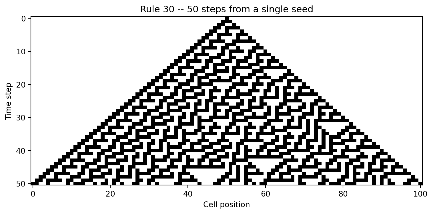
#| fig-cap: "Rule 30 space-time diagram: 50 steps from a single live cell, generating a chaotic asymmetric pattern with no visible period."
import matplotlib.pyplot as plt
grid30 = run_ca(30, steps=50, width=101)
fig, ax = plt.subplots(figsize=(8, 4))
ax.imshow(grid30, cmap='binary',
interpolation='nearest', aspect='auto')
ax.set_title('Rule 30 -- 50 steps from a single seed')
ax.set_xlabel('Cell position')
ax.set_ylabel('Time step')
plt.tight_layout()
plt.show()
```
Run this. The result is striking: a chaotic, asymmetric pattern
with no visible period and no obvious symmetry -- produced by
eight numbers in a table.
## Rule 30: A Natural Random Number Generator {#sec-automata-rule30}
Rule 30 is one of the most famous elementary CAs. Its space-time
diagram looks genuinely random: no stripes, no blocks, no
symmetry. Wolfram showed that the **central column** of Rule 30
-- the sequence of values at the starting cell across all time
steps -- passes many standard statistical tests for randomness.
For years, Wolfram's *Mathematica* software used this sequence
as its built-in random-integer generator [@wolfram1986random].
Let us check the balance of 0s and 1s in the central column:
```{python}
grid30_long = run_ca(30, steps=1000, width=2001)
center_pos  = 2001 // 2

central_col = [row[center_pos] for row in grid30_long]
ones  = central_col.count(1)
zeros = central_col.count(0)
total = len(central_col)
print(f"Steps : {total}")
print(f"Ones  : {ones}  ({100 * ones / total:.2f}%)")
print(f"Zeros : {zeros}  ({100 * zeros / total:.2f}%)")
```
The output shows roughly equal counts of 0s and 1s -- a key
property of a good random bit source.
We can push further and test whether consecutive bits are
independent. If the sequence were truly random, transitions
(a bit changing from 0 to 1 or 1 to 0) and non-transitions
(consecutive equal bits) should each appear about 50% of the
time.
```{python}
transitions = sum(
    1 for i in range(1, len(central_col))
    if central_col[i] != central_col[i - 1]
)
pct = 100 * transitions / (len(central_col) - 1)
print(f"Transitions    : {transitions}")
print(f"Transition rate: {pct:.2f}%  (ideal: 50.00%)")
```
Rule 30's central column is **not** cryptographically secure:
given enough output bits, one can reconstruct the entire grid
and predict all future values. Real cryptographic generators
need additional security properties. But for simulation work --
generating random numbers for scientific models -- Rule 30
performs well and runs extremely fast.
### Research Example: Which Rule Forgets a Flipped Bit? {.unnumbered .unlisted}
If two copies of a rule begin from rows that differ in exactly one cell, how fast does
that difference spread? A chaotic rule should amplify the gap almost instantly; an
ordered rule might hold it frozen in place. We track the **Hamming distance** — the
count of positions where two parallel runs disagree — across 100 time steps to catch
each rule's reaction to a one-cell perturbation.
```{python}
#| label: fig-ca-hamming
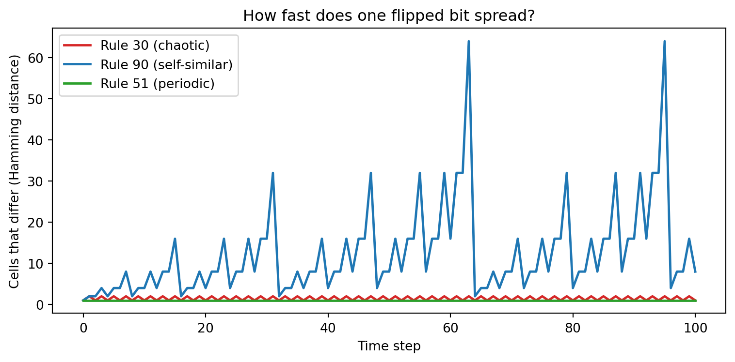
#| fig-cap: "Hamming distance between two runs that start one cell apart: Rule 30 explodes to near-maximum within 30 steps, Rule 90 bounces in irregular powers of two reflecting its Sierpiński structure, and Rule 51 keeps the distance frozen at exactly 1 forever because its complement symmetry is a linear map that preserves any initial gap."
# uses: apply_rule()
BLUE  = '#1f77b4'
RED   = '#d62728'
GREEN = '#2ca02c'
import matplotlib.pyplot as plt

width = 201
base      = [0] * width
base[width // 2] = 1
perturbed = base[:]
perturbed[width // 2 + 1] = 1   # one extra live cell

steps = 100
fig, ax = plt.subplots(figsize=(8, 4))
for rule, color, label in [
    (30, RED,   'Rule 30 (chaotic)'),
    (90, BLUE,  'Rule 90 (self-similar)'),
    (51, GREEN, 'Rule 51 (periodic)'),
]:
    a, b = base[:], perturbed[:]
    dist = [sum(x != y for x, y in zip(a, b))]
    for _ in range(steps):
        a = apply_rule(a, rule)
        b = apply_rule(b, rule)
        dist.append(sum(x != y for x, y in zip(a, b)))
    ax.plot(dist, color=color, label=label, linewidth=1.8)

ax.set_xlabel('Time step')
ax.set_ylabel('Cells that differ (Hamming distance)')
ax.set_title('How fast does one flipped bit spread?')
ax.legend()
plt.tight_layout()
plt.show()
```
Rule 30 races to near-maximum disagreement within 30 steps and never recovers — that
single extra live cell is enough to make the two runs look completely unrelated, which
is precisely what "sensitive dependence on initial conditions" means for a deterministic
system. Rule 90 bounces up and down in jumps that are always powers of two, a fractal
fingerprint of the Sierpiński pattern hiding inside its XOR rule. Rule 51 freezes the
distance at exactly 1 forever, because complementing every cell is a linear operation
that maps any difference to the same difference at every step: ordered rules carry
perturbations, they do not amplify them. One flipped bit, three completely different
reactions — written in a single curve.
## Rule 90 and Pascal's Triangle {#sec-automata-rule90}
Rule 90 has a completely different character. Verify its table:
```{python}
show_rule_table(90)
```
The output column for Rule 90 is 0 1 0 1 1 0 1 0, which equals
$01011010_2 = 90_{10}$. Notice the pattern: the output is 1
when $L \ne R$, and 0 when $L = R$. In other words,
$$\text{new}[i] = L \oplus R$$
where $\oplus$ denotes XOR (exclusive-or): output 1 when the
inputs differ, 0 when they match. **The center cell is completely
ignored.**
```{python}
#| label: fig-ca-rule90
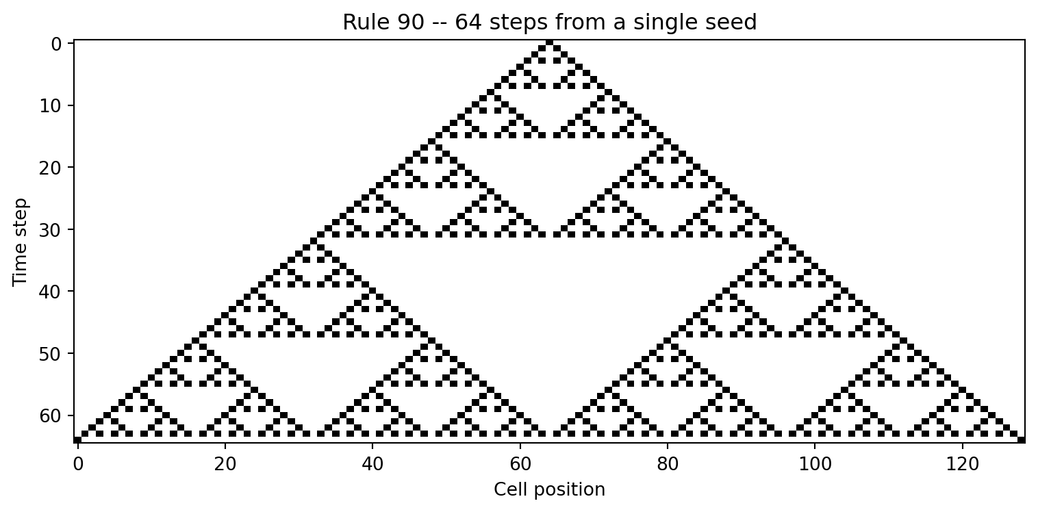
#| fig-cap: "Rule 90 space-time diagram: 64 steps from a single seed, producing a pattern identical to the Sierpinski triangle from Pascal's triangle mod 2."
grid90 = run_ca(90, steps=64, width=129)

fig, ax = plt.subplots(figsize=(8, 4))
ax.imshow(grid90, cmap='binary',
          interpolation='nearest', aspect='auto')
ax.set_title('Rule 90 -- 64 steps from a single seed')
ax.set_xlabel('Cell position')
ax.set_ylabel('Time step')
plt.tight_layout()
plt.show()
```
This diagram should look very familiar. Compare it to the
Sierpinski triangle generated from Pascal's triangle mod 2 in
@sec-pascal-sierpinski. The two images appear identical.
The connection is exact. Starting from a single 1 at position
$c$, after $t$ steps the cell at position $c + k$ is alive if
and only if $\binom{t}{(t+k)/2}$ is odd -- and that is
precisely the Sierpinski pattern from Chapter 6. (Note that
$(t + k)$ must be even; odd-parity positions are always 0.)
We can verify this computationally:
```{python}
import math

width  = 129
center = width // 2
grid90 = run_ca(90, steps=64, width=width)

mismatches = 0
for t in range(65):
    for k in range(-t, t + 1):
        if (t + k) % 2 != 0:
            pascal_val = 0
        else:
            j = (t + k) // 2
            pascal_val = math.comb(t, j) % 2
        ca_val = grid90[t][center + k]
        if ca_val != pascal_val:
            mismatches += 1

print(f"Mismatches (Rule 90 vs Pascal mod 2): {mismatches}")
```
Output: `Mismatches (Rule 90 vs Pascal mod 2): 0`.
Two completely different definitions -- one based on XOR of
neighbors, one based on counting paths in a triangle -- produce
the exact same pattern. Why?
The XOR operation satisfies the same recurrence as addition
mod 2. If $x_t(i)$ denotes the value of cell $i$ at time $t$,
then Rule 90 gives $x_{t+1}(i) = x_t(i-1) + x_t(i+1) \pmod 2$.
Over the integers mod 2, this linear recurrence has the same
solution as Pascal's triangle: $x_t(c + k) = \binom{t}{(t+k)/2}
\bmod 2$ for even $t + k$.
This is a deeper pattern than either the CA or the triangle
could reveal on its own -- one of those hidden identities that
experimental mathematics is ideally suited to discover
[@borwein2006ema, §3.2].
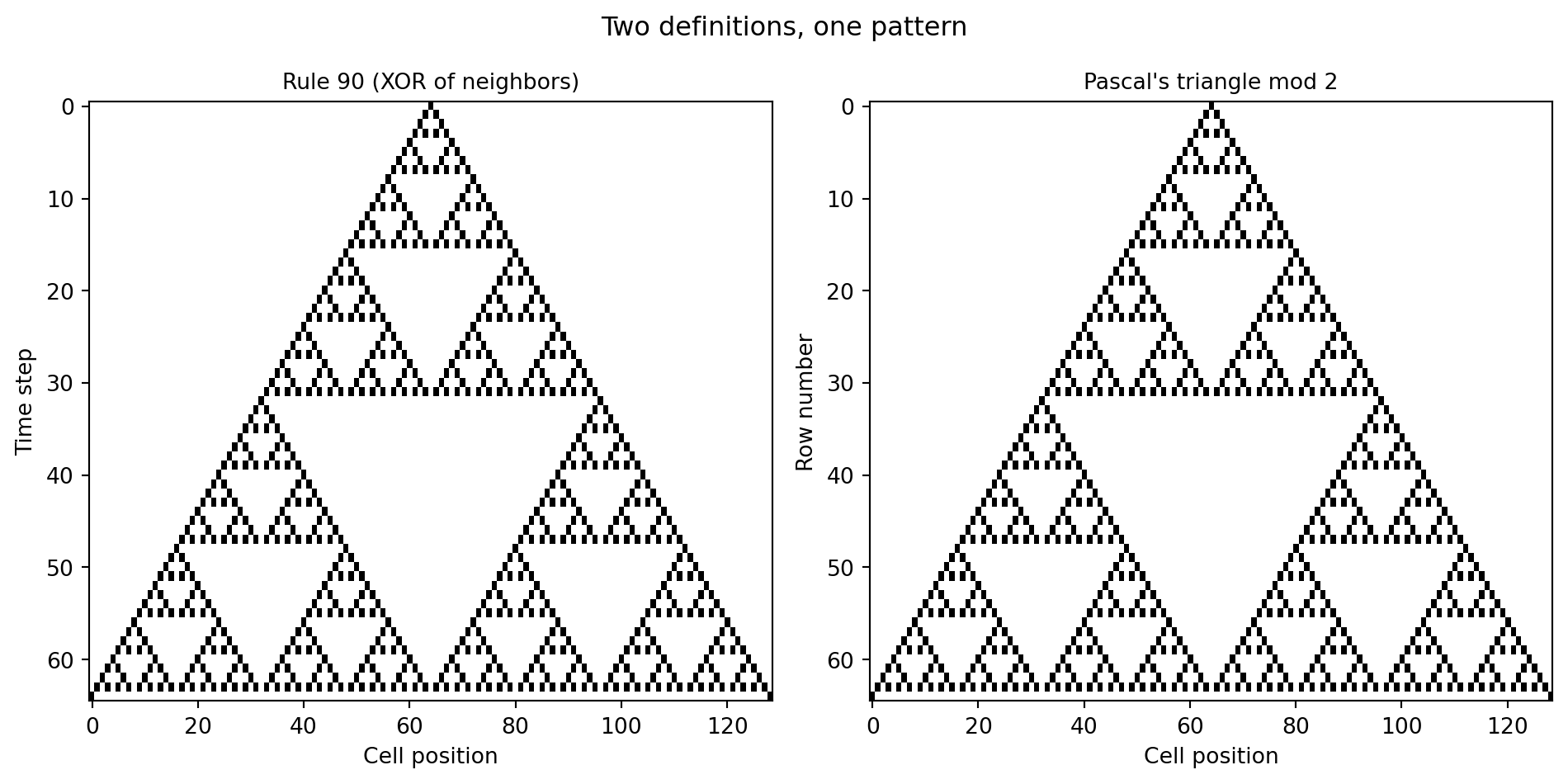
### Research Example: Can You See the Pascal Connection? Two Pictures, One Pattern {.unnumbered .unlisted}
The code above printed zero mismatches — but a single number is easy to scroll past. A picture is harder to dismiss. If Rule 90 and Pascal's triangle mod 2 are truly the same pattern, they should produce an image that is pixel-for-pixel identical from both constructions. Let us put them side by side.
```{python}
#| label: fig-ca-pascal-compare
#| fig-cap: "Left: Rule 90 run 64 steps from a single seed. Right: Pascal's triangle entries mod 2 on the same grid. Black = 1, white = 0. The panels are pixel-for-pixel identical — XOR of neighbors and parity of a binomial coefficient give exactly the same answer."
import math
import matplotlib.pyplot as plt

steps  = 64
width  = 129
center = width // 2

grid90 = run_ca(90, steps=steps, width=width)

pascal_grid = []
for t in range(steps + 1):
    row = []
    for i in range(width):
        k = i - center
        if abs(k) > t or (t + k) % 2 != 0:
            row.append(0)
        else:
            row.append(math.comb(t, (t + k) // 2) % 2)
    pascal_grid.append(row)

fig, axes = plt.subplots(1, 2, figsize=(10, 5))
axes[0].imshow(grid90, cmap='binary',
               interpolation='nearest', aspect='auto')
axes[0].set_title('Rule 90 (XOR of neighbors)', fontsize=10)
axes[0].set_xlabel('Cell position')
axes[0].set_ylabel('Time step')

axes[1].imshow(pascal_grid, cmap='binary',
               interpolation='nearest', aspect='auto')
axes[1].set_title("Pascal's triangle mod 2", fontsize=10)
axes[1].set_xlabel('Cell position')
axes[1].set_ylabel('Row number')

plt.suptitle('Two definitions, one pattern', fontsize=12)
plt.tight_layout()
plt.show()
```
Two completely different operations — XOR-ing a cell's left and right neighbors versus checking whether a binomial coefficient is even or odd — produce images that cannot be told apart by eye or by computer. Hidden inside Rule 90 is an entire chapter of combinatorics.
## Symmetry Classes {#sec-automata-symmetry}
Not all rules are equally complex. Wolfram observed that the
256 elementary CA rules fall into **four classes** based on
the long-run behavior of their space-time diagrams [@wolfram2002, Ch. 6].
- **Class 1 (uniform):** The pattern quickly dies or fills
completely. All activity disappears after a few steps.
*Example: Rule 0* (every neighborhood maps to 0;
the entire row dies after one step).
- **Class 2 (periodic):** The pattern stabilizes into
repeating stripes or blocks with a fixed period.
*Example: Rule 51* (maps every pattern to its complement;
the row oscillates with period 2).
- **Class 3 (chaotic):** The pattern appears random and
aperiodic. Small changes to the initial state cause large
differences later. *Example: Rule 30*.
- **Class 4 (complex):** The pattern produces localized
structures -- called **particles** or **gliders** -- that
persist, move, and interact. This is the rarest class.
*Example: Rule 110*.
::: {.content-visible when-format="pdf"}
```{=latex}
\begin{center}
\begin{minipage}[c]{0.22\textwidth}
\includegraphics[width=\textwidth]{images/matthew-cook.jpg}
\end{minipage}%
\hspace{0.03\textwidth}%
\begin{minipage}[c]{0.55\textwidth}
\small\textit{Matthew Cook (b.\ 1970)}\\[2pt]
\tiny Photo: \url{https://www.ini.uzh.ch/}
\end{minipage}
\end{center}
```
:::
::: {.content-visible when-format="html"}
<div style="display:flex; align-items:center; margin:1em 0; gap:12px;">
<img src="images/matthew-cook.jpg" style="width:100px; flex-shrink:0;" alt="Matthew Cook">
<div style="font-size:0.82em;"><em>Matthew Cook (b. 1970)</em><br><span style="font-size:0.85em;">Photo: <a href="https://www.ini.uzh.ch/">ini.uzh.ch</a></span></div>
</div>
:::
Rule 110 occupies a special place in the history of
computation. Matthew Cook proved in 2004 that Rule 110 is
**Turing-complete**: it can simulate any computation that any
digital computer can perform [@cook2004].
Universal computation is hiding inside a rule defined by eight
bits.
To see all four classes at once, we run each from the same
random initial state:
```{python}
#| label: fig-ca-classes
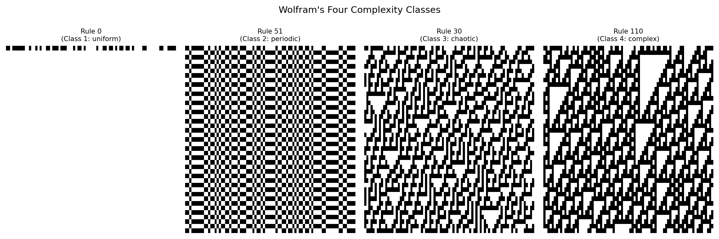
#| fig-cap: "Wolfram's four complexity classes run from the same random initial condition: immediate death (Rule 0), periodic oscillation (Rule 51), computational chaos (Rule 30), and complex glider dynamics (Rule 110)."
import random

random.seed(0)
width = 81
init_random = [random.randint(0, 1) for _ in range(width)]

def run_ca_from(rule_num, init, steps):
    cells = init[:]
    grid  = [cells[:]]
    for _ in range(steps):
        cells = apply_rule(cells, rule_num)
        grid.append(cells[:])
    return grid

rules  = [0, 51, 30, 110]
labels = [
    'Rule 0\n(Class 1: uniform)',
    'Rule 51\n(Class 2: periodic)',
    'Rule 30\n(Class 3: chaotic)',
    'Rule 110\n(Class 4: complex)',
]

fig, axes = plt.subplots(1, 4, figsize=(12, 4))
for ax, rule, label in zip(axes, rules, labels):
    grid = run_ca_from(rule, init_random, steps=40)
    ax.imshow(grid, cmap='binary',
              interpolation='nearest', aspect='auto')
    ax.set_title(label, fontsize=8)
    ax.axis('off')
plt.suptitle(
    "Wolfram's Four Complexity Classes",
    fontsize=11
)
plt.tight_layout()
plt.show()
```
The four panels tell the whole story at a glance: immediate
death, checkerboard oscillation, a chaotic ocean, and living
structures navigating each other.
The 256 rules contain further hidden structure through symmetry.
Reflecting a rule left-to-right produces its **mirror rule**
(Rule 30's mirror is Rule 86: swap the outputs for every pair
of patterns $LCR$ and $RCL$). Swapping the roles of 0 and 1
produces the **complement rule** (Rule 30's complement is Rule
135). These two symmetries, together with their composition,
divide the 256 rules into just **88 truly distinct families**.
Rules in the same family have the same complexity class and
produce the same patterns up to reflection or color-swap.
## The Entropy Landscape {#sec-automata-entropy}
How do you put a single number on "how complicated" a pattern
looks? Information theorist Claude Shannon gave us a tool in
1948: **Shannon entropy** [@shannon1948]. For a row where a fraction $p$ of
cells are alive, the row entropy is
$$H = -p\log_2 p - (1-p)\log_2(1-p)$$
$H$ equals 0 when a row is all-dead or all-alive (completely
predictable) and reaches its maximum of 1 bit when exactly half
the cells are alive (maximally uncertain). A Class 1 rule that
kills everything should drive $H \to 0$; a genuinely random
Class 3 rule should keep $H$ close to 1.
Numbers beat words. We run all 256 rules from the same random
starting row for 100 steps and record the mean row entropy over
the last 50 steps -- letting the initial transient die down
before we measure:
```{python}
#| label: fig-ca-entropy
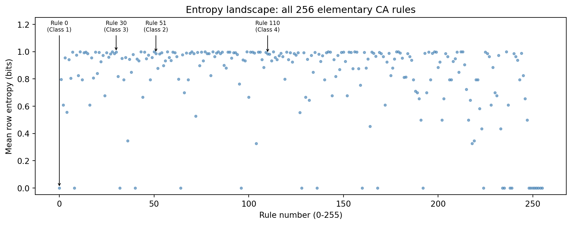
#| fig-cap: "Mean row Shannon entropy for all 256 elementary CA rules, run from the same random initial condition. Class 1 rules collapse to near-zero entropy; most Class 2, 3, and 4 rules cluster near 1 bit."
def row_entropy(row):
    n = len(row)
    p = sum(row) / n
    if p == 0 or p == 1:
        return 0.0
    return (
        -p * math.log2(p)
        - (1 - p) * math.log2(1 - p)
    )

random.seed(42)
width_e = 201
init_e = [
    random.randint(0, 1) for _ in range(width_e)
]

mean_H = []
for r in range(256):
    grid_e = run_ca_from(r, init_e, steps=100)
    last50 = grid_e[51:]
    H_vals = [row_entropy(row) for row in last50]
    mean_H.append(sum(H_vals) / len(H_vals))

fig, ax = plt.subplots(figsize=(10, 4))
ax.scatter(
    range(256), mean_H,
    s=8, alpha=0.6, color='steelblue'
)
ax.set_xlabel('Rule number (0-255)')
ax.set_ylabel('Mean row entropy (bits)')
ax.set_ylim(-0.05, 1.25)
ax.set_title(
    'Entropy landscape: all 256 elementary CA rules'
)

labels_ann = [
    (0,   'Rule 0\n(Class 1)'),
    (51,  'Rule 51\n(Class 2)'),
    (30,  'Rule 30\n(Class 3)'),
    (110, 'Rule 110\n(Class 4)'),
]
for rule_n, lbl in labels_ann:
    h = mean_H[rule_n]
    ax.annotate(
        lbl,
        xy=(rule_n, h),
        xytext=(rule_n, 1.15),
        fontsize=7,
        ha='center',
        arrowprops=dict(arrowstyle='->', lw=0.8),
    )

plt.tight_layout()
plt.show()
```
The scatter plot is a fingerprint of the entire 256-rule
universe. Class 1 rules drop straight to zero -- the pattern
dies, entropy vanishes. The rest pile up near 1 bit.
Notice something surprising: Rule 51 (Class 2: periodic) sits
just as high as Rule 30 (Class 3: chaotic). Why? Rule 51 flips
every cell at every step. Starting from a random row where about
half the cells are alive, flipping all of them leaves about half
alive -- so the density stays near 50% forever, keeping
$H \approx 1$. The pattern is perfectly predictable (just
alternate between two states), yet entropy cannot see that.
This is the key limitation of entropy as a classifier: it
measures *density* unpredictability, not *structural* complexity.
It cleanly separates Class 1 from the rest, but cannot
distinguish periodic from chaotic from complex. To separate
those, you need richer statistics -- the kind you can design in
the research topics below.
### Research Example: How Quickly Does Each Wolfram Class Reach Its Entropy Ceiling? {.unnumbered .unlisted}
The scatter plot above shows where each rule ends up — but not how it gets there. Class 1 collapses instantly; do the other three classes climb at the same speed? Plotting entropy at every time step, rather than averaging, reveals the dynamical signature hiding inside each class.
```{python}
#| label: fig-ca-entropy-time
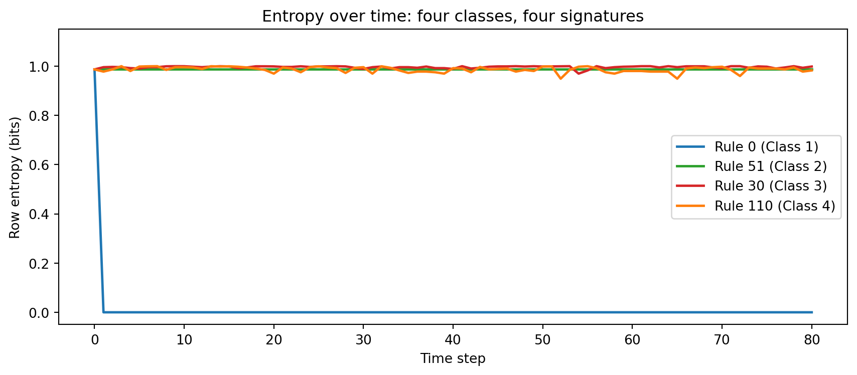
#| fig-cap: "Shannon entropy per row at every time step, for one representative rule from each Wolfram class. Class 1 (Rule 0) reaches zero in a single step. Class 2 (Rule 51) oscillates between two fixed values. Class 3 (Rule 30) erupts to near-1 bit within 10 steps and locks in. Class 4 (Rule 110) climbs slowly to an intermediate plateau — a subtler, more structured texture than pure chaos."
import matplotlib.pyplot as plt
import random

BLUE   = '#1f77b4'
GREEN  = '#2ca02c'
RED    = '#d62728'
ORANGE = '#ff7f0e'

random.seed(42)
width_t = 201
init_t  = [random.randint(0, 1) for _ in range(width_t)]

class_rules  = [0,    51,    30,    110]
class_labels = ['Rule 0 (Class 1)', 'Rule 51 (Class 2)',
                'Rule 30 (Class 3)', 'Rule 110 (Class 4)']
class_colors = [BLUE, GREEN, RED, ORANGE]

fig, ax = plt.subplots(figsize=(9, 4))
for rule, label, color in zip(class_rules, class_labels, class_colors):
    grid_t = run_ca_from(rule, init_t, steps=80)
    H_vals = [row_entropy(row) for row in grid_t]
    ax.plot(H_vals, label=label, color=color, linewidth=1.8)

ax.set_xlabel('Time step')
ax.set_ylabel('Row entropy (bits)')
ax.set_title('Entropy over time: four classes, four signatures')
ax.legend(loc='right')
ax.set_ylim(-0.05, 1.15)
plt.tight_layout()
plt.show()
```
Each class leaves a distinct temporal fingerprint. Rule 0 kills the pattern in a single step — entropy drops to zero and never recovers. Rule 51 stays locked near 1 bit despite being perfectly periodic: flipping every cell at every step preserves the 50-50 balance, so density never changes, and entropy cannot see the pattern's regularity. Rule 30 erupts to near-maximum entropy within a handful of steps and stays there — the signature of genuine chaos. Rule 110 climbs slowly and plateaus slightly below Rule 30, reflecting the structured-but-not-uniform texture of glider dynamics. The gap between Rule 110 and Rule 30 is the one place entropy gives a hint that something subtler is happening.
## Further Research Topics {#sec-automata-research}
The topics below progress from straightforward experiments to
open research questions.
1. **Counting live cells per generation.** For each rule 0--255,
run the CA for 50 steps from a single seed and record the
number of live cells at each step. Which rules produce linear
growth in live-cell count? Quadratic? Which oscillate? Can
you predict the growth pattern from the rule number alone,
or must you simulate? *(Problem proposed by Claude Code.)*
2. **Mirror and complement symmetry.** The mirror of rule $r$
is formed by swapping outputs for every pair of patterns
$LCR$ and $RCL$ (e.g. swap the outputs for 100 and 001,
swap 110 and 011, keep 000 and 111 fixed). Write a function
`mirror_rule(r)` and verify that `mirror_rule(30) == 86`.
How many of the 256 rules are self-mirror (equal to their own
mirror)? How many are self-complement? How many are both?
*(Problem proposed by Claude Code.)*
3. **Shannon entropy as a complexity meter.** For each row of a
space-time diagram define the row entropy
$H = -p\log_2 p - (1-p)\log_2(1-p)$, where $p$ is the
fraction of live cells in that row ($H = 0$ when $p = 0$
or $p = 1$, and $H = 1$ when $p = 0.5$). Run every rule
0--255 for 100 steps from the same random initial condition
and compute the mean row entropy over the last 50 steps.
Plot mean entropy against rule number. Do Wolfram's four
classes cluster at distinct entropy levels? Class 1 should
give $H \approx 0$; what do Classes 2, 3, and 4 predict?
Use mean entropy alone as a one-feature classifier and
measure how often it correctly assigns a rule to the right
class. *(Problem proposed by Claude Code.)*
4. **Frequency tests on Rule 30's central column.** Apply the
chi-squared digit-frequency test from @sec-constants-normal
to the central column of Rule 30. Does it pass at the 5%
significance level? Extend the test: are all four two-bit
patterns (00, 01, 10, 11) equally common? All eight three-bit
patterns? At what run length does the test first detect
non-uniformity, if ever? Compare to Rule 90's central column.
*(Problem proposed by Claude Code.)*
5. **Classifying all 256 rules automatically.** Run every rule
0--255 for 100 steps from the same random initial condition.
Record (a) the number of live cells in the final row, (b)
whether the last 10 rows are periodic, and (c) the variance
in live-cell count across the last 50 rows. Use these three
numbers to cluster the rules with Python's `statistics`
module. How well does your automated clustering match
Wolfram's four-class taxonomy? *(Problem proposed by Claude Code.)*
6. **Totalistic rules.** In a **totalistic** CA the new state
depends only on the three-cell sum (0, 1, 2, or 3), not on
the positions of the 1s. There are $2^4 = 16$ outer
totalistic rules (new state depends on center + sum of
neighbors). Write `apply_totalistic(cells, rule_num)` and
explore all 16. Which classes appear? How does the totalistic
family relate to the full 256-rule elementary family?
*(Problem proposed by Claude Code.)*
7. **Langton's lambda and the edge of chaos** [@langton1990]**.** Langton's
parameter $\lambda$ is the fraction of the 8 output bits
in a rule that equal 1. Compute $\lambda$ for all 256 rules
and plot mean row entropy (from topic 3) against $\lambda$.
Langton's conjecture says complexity peaks near $\lambda =
0.5$ -- the "edge of chaos" between ordered and disordered
behavior. Does your scatter plot support this? Which Wolfram
classes cluster near $\lambda = 0$ or $\lambda = 1$, and
which appear near $\lambda = 0.5$? Is $\lambda$ a better
predictor of class than the rule number itself?
*(Problem proposed by Claude Code.)*
8. **Sensitive dependence and the Lyapunov exponent.** Start
two copies of Rule 30 with identical rows except that one
cell is flipped. At each step, count the number of positions
where the two runs differ (the **Hamming distance**). Plot
Hamming distance vs. time on a log scale. If the growth is
exponential, fit a line to estimate a spreading rate
analogous to the Lyapunov exponent in the logistic map
(Chapter 11). Repeat for Rule 90 and Rule 51. What does
each class predict about this spreading rate?
*(Problem proposed by Claude Code.)*
9. **Reversible cellular automata.** A CA is *reversible* if
every past state can be recovered from the present state
alone. The *second-order* construction
$x_{t+1}(i) = f\!\bigl(x_t(i{-}1),\,x_t(i),\,x_t(i{+}1)\bigr)
\oplus x_{t-1}(i)$
produces a reversible rule from any elementary rule $f$:
given rows $t$ and $t{+}1$, row $t{-}1$ equals
$f(\text{neighborhood at }t) \oplus x_{t+1}(i)$.
Implement `run_reversible_ca(rule_num, steps)` that stores
two consecutive rows and iterates forward, then write
`reverse_ca(grid)` that runs the grid backward by treating
row $t{+}1$ as "past." Verify that running 100 steps forward
and then 100 steps backward recovers the original seed
exactly. Which elementary rules produce periodic behavior
when made reversible, and which remain aperiodic?
*(Problem proposed by Claude Code.)*
10. **Initial conditions and universality.** Run Rule 110 from
10 different random initial conditions (change `random.seed`).
Does the long-run behavior always look complex, or does the
initial condition matter? Now run Rule 30 from 10 different
random seeds. Do all seeds produce chaotic-looking patterns?
Formulate a conjecture: is the class of a rule a property
of the rule alone, or can a rule behave differently for
different initial conditions? *(Problem proposed by Claude Code.)*
11. **The 88 equivalence classes in detail.** Generate the full
equivalence-class list: for each of the 256 rules, compute
its mirror, complement, and mirror-complement; group together
all four into one family. Print each family with its four
members (or fewer, if any members coincide). How many
families have size 1? Size 2? Size 4? Identify a familiar
algebraic structure that explains the family sizes.
*(Problem proposed by Claude Code.)*
12. **Two-color, five-cell neighborhoods.** Extend the elementary
CA idea to a five-cell neighborhood (two cells on each side).
There are $2^5 = 32$ patterns and $2^{32} \approx 4$ billion
possible rules -- far too many to classify by hand. Write a
five-cell simulator. Starting from a single seed, find one
rule in this family that produces a pattern whose alive cells
at time $t$ match $\binom{t}{k} \bmod 2$ for some analogous
formula (a "Pascal-like" identity). Hint: look for rules
where the output depends only on the XOR of the outermost
pair and some function of the inner three.
*(Problem proposed by Claude Code.)*
13. **Three-color totalistic rules.** Extend the state space to
$\{0, 1, 2\}$. In a *three-state inner totalistic* CA the
new state depends only on the sum of the three-cell
neighborhood (ranging from 0 to 6), so each sum maps to
one of three outputs, giving $3^7 = 2{,}187$ possible rules.
Write a three-state totalistic simulator. Explore a sample
of rules: can you find one whose space-time diagram is
self-similar (a Sierpinski-like fractal)? One that appears
genuinely random? Wolfram's "code 777" in the three-state
totalistic numbering is especially famous for apparent
chaos -- implement and visualize it. How many distinct
Wolfram-like classes can you identify across this larger
family? *(Problem proposed by Claude Code.)*
14. **Fractal dimension by box-counting.** Rule 90's space-time
diagram is the Sierpinski triangle, whose fractal dimension
is $\log_2 3 \approx 1.585$ (see @sec-pascal-sierpinski) [@wolfram2002, Ch. 5].
Estimate the fractal dimension of Rule 30's space-time
diagram using the *box-counting* method: tile the diagram
with a grid of boxes of side $\epsilon$ and count
$N(\epsilon)$ boxes that contain at least one live cell.
Repeat for $\epsilon = 2, 4, 8, 16, 32, 64$. Plot
$\log N(\epsilon)$ vs.\ $\log(1/\epsilon)$ and fit a
straight line; its slope estimates the fractal dimension.
Calibrate your method by checking that it gives a value
near $\log_2 3$ for Rule 90. Is Rule 30's pattern a fractal?
Does its estimated dimension change if you use a different
random seed for the initial condition? *(Problem proposed by Claude Code.)*
15. **Gliders in Rule 110.** In Class 4 rules, small localized
patterns can move across the grid without changing shape
(called **gliders**). Run Rule 110 on a wide grid (width
>= 600, steps >= 400) from a carefully chosen initial
pattern. Search for a repeating, translating structure.
Document one glider by showing its cell pattern at
consecutive time steps, measuring its period (how many
steps before the shape repeats) and its velocity (cells
per step). Could two such gliders collide? Simulate it
and describe what happens. *(Problem proposed by Claude Code.)*
16. **Conway's Game of Life** [@conway1970]**.** Extend the CA idea to two
dimensions: each cell has 8 neighbors (the Moore
neighborhood). A live cell with 2 or 3 live neighbors
survives; all other live cells die. A dead cell with
exactly 3 live neighbors becomes alive. Implement this in
Python using a 2D list. Find the "glider" (a five-cell
pattern that moves diagonally one cell every 4 steps).
Verify that Conway's Game of Life is Turing-complete --
what does that imply about the relationship between rule
complexity and computational power? *(Problem proposed by Claude Code.)*
17. **Statistical fingerprinting.** Can you identify the class
of an unknown rule from its statistics alone, without
looking at the diagram? Build a feature vector for each
rule: (mean live-cell density, variance, longest run
of same value in a row, transition rate in central column,
Hamming distance growth rate). Train a simple nearest-
neighbor classifier to assign each of the 256 rules to
one of Wolfram's four classes. What is the classification
accuracy? Which rules are hardest to classify, and why?
*(Problem proposed by Claude Code.)*
18. **Transition matrix over GF(2).** Rule 90's evolution
$x_{t+1}(i) = x_t(i{-}1) \oplus x_t(i{+}1)$ is *linear*:
it can be written as matrix multiplication over
$\mathrm{GF}(2)$, the field where $1 + 1 = 0$.
For a grid of width $n$ with periodic boundary conditions,
the transition matrix $A$ is the $n \times n$ circulant
matrix with 1s at positions $(i,\,i{-}1 \bmod n)$ and
$(i,\,i{+}1 \bmod n)$ and 0s elsewhere.
Implement matrix-vector multiplication modulo 2 using
Python lists and verify that $A\mathbf{v} \pmod 2$ matches
`apply_rule(cells, 90)` on the same initial state
$\mathbf{v}$.
Compute $A^2, A^4, A^8, \ldots$ by repeated squaring
modulo 2.
Find the smallest $k$ such that $A^{2^k}$ is the identity
(meaning Rule 90 returns every initial state to itself
after $2^k$ steps).
How does this $k$ depend on the grid width $n$?
Is something special about widths that are powers of 2?
*(Problem proposed by Claude Code.)*
19. **Self-replicating patterns and Garden-of-Eden states.**
A *Garden-of-Eden* configuration can never be reached from
any predecessor -- it exists only as an initial condition.
A *self-replicating* pattern produces at least one complete
copy of itself after some number of steps. In Conway's Game
of Life (topic 16), the Gosper glider gun fires a new
glider every 30 generations [@berlekamp1982]. Write a function
`count_pattern(grid, pattern)` that searches a large grid
for all occurrences of a small pattern at time $T$. Starting
from the Gosper glider gun initial configuration, count
the number of gliders present at steps 100, 200, and 300.
Does the count grow linearly? Prove or disprove it
algebraically. Then turn to 1D: can you find any elementary
CA rule and initial condition such that the initial pattern
reappears (perhaps shifted) somewhere in the grid after a
finite number of steps? *(Problem proposed by Claude Code.)*
20. **Cellular automata as music.** Map a CA space-time diagram
to a musical score: assign each column of the grid to a
pitch in the chromatic scale (12 notes per octave, repeated
across as many octaves as needed), and let each row
represent one beat. A live cell means "play this note," a
dead cell means "rest." Write a function that converts a
CA grid to a sequence of (pitch, duration) pairs and saves
it as a MIDI file using the `midiutil` library
(`pip install midiutil`). Generate pieces from Rule 30
(chaotic), Rule 90 (self-similar), Rule 110 (complex),
and Rule 51 (periodic). Which sounds most like structured
music? Which sounds most random? Experiment with mapping
the *row density* to tempo or dynamics. Can you choose an
initial condition for Rule 110 that makes the resulting
piece contain a recognizable repeating motif? This connects
to a genuine research area: algorithmic composition using
deterministic dynamical systems. *(Problem proposed by Claude Code.)*