# Integer Sequences and the OEIS {#sec-oeis}
Neil Sloane began collecting integer sequences on punched cards in
1964 as a graduate student at Cornell. By the time his database
moved online in 1996, it held tens of thousands of entries. Today
the Online Encyclopedia of Integer Sequences (OEIS) contains over
370,000 sequences, each one a numbered window into a different
corner of mathematics. This chapter shows how to generate and
analyze sequences in Python, then use the OEIS to turn a mystery
list of numbers into a research project.
## What Is a Sequence? {#sec-oeis-intro}
An *integer sequence* is a list of integers indexed by position:
$a(1), a(2), a(3), \ldots$ or $a(0), a(1), a(2), \ldots$ depending
on convention. Three styles of definition appear throughout
mathematics.
**Closed form.** A formula gives $a(n)$ directly from $n$. The
square numbers satisfy $a(n) = n^2$; any term is instant to compute.
**Recurrence.** Each term is defined in terms of earlier terms. The
Fibonacci sequence (see @sec-fib-rabbits) satisfies
$F(n) = F(n-1) + F(n-2)$ with $F(1) = F(2) = 1$; you must build
the list from the start to reach any term.
**Algorithm.** A procedure generates each term but no compact
formula is known. The prime sequence (see @sec-primes-sieve)
requires testing each candidate for divisibility.
Python handles all three naturally.
```{python}
from sympy import primerange

# closed form: squares
squares = [n**2 for n in range(1, 11)]
print("squares:  ", squares)

# recurrence: Fibonacci
fib = [1, 1]
while len(fib) < 10:
    fib.append(fib[-1] + fib[-2])
print("fibonacci:", fib)

# algorithm: primes below 30
primes_10 = list(primerange(2, 30))
print("primes:   ", primes_10)
```
Generating the first dozen or so terms of a sequence is usually
enough to search for it in the OEIS. This short prefix -- a
*fingerprint* -- is your primary search key.
## The OEIS {#sec-oeis-database}
::: {.content-visible when-format="pdf"}
```{=latex}
\begin{center}
\begin{minipage}[c]{0.28\textwidth}\centering
\href{https://youtu.be/OeGSQggDkxI}{\includegraphics[width=\textwidth]{images/thumb_OeGSQggDkxI.jpg}}
\end{minipage}%
\hspace{0.02\textwidth}%
\begin{minipage}[c]{0.28\textwidth}
\small\textbf{Numberphile}\\[3pt]
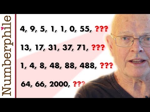
\small What Number Comes Next? (feat.\ Neil Sloane)\\[3pt]
\small\href{https://youtu.be/OeGSQggDkxI}{\texttt{youtu.be/OeGSQggDkxI}}
\end{minipage}%
\hspace{0.02\textwidth}%
\begin{minipage}[c]{0.36\textwidth}
\small Neil Sloane — founder of the OEIS — explains how the database came to be and why a shared library of number sequences is an essential tool for mathematical research.
\end{minipage}
\end{center}
```
:::
::: {.content-visible when-format="html"}
<div style="display:flex; align-items:flex-start; margin:1em 0; gap:12px; width:100%;">
<div style="flex:0 0 200px;"><a href="https://youtu.be/OeGSQggDkxI" target="_blank"><img src="https://img.youtube.com/vi/OeGSQggDkxI/0.jpg" style="width:100%;" alt="What Number Comes Next?"></a></div>
<div style="flex:1; font-size:0.85em;"><strong>Numberphile</strong><br>What Number Comes Next? (feat. Neil Sloane)<br><a href="https://youtu.be/OeGSQggDkxI" target="_blank" style="font-family:monospace;">youtu.be/OeGSQggDkxI</a></div>
<div style="flex:1; font-size:0.85em;">Neil Sloane — founder of the OEIS — explains how the database came to be and why a shared library of number sequences is an essential tool for mathematical research.</div>
</div>
:::
The OEIS lives at oeis.org. Each entry has a unique identifier
called an *A-number*, such as A000040 (prime numbers) or A000045
(Fibonacci numbers). A typical entry contains:
- the first several hundred or thousand terms
- a formula or recurrence
- references to books and papers
- links to related sequences
- programs in various languages that generate it
To search, paste the first several terms -- separated by commas --
into the search box. Entering "2, 3, 5, 7, 11, 13" returns A000040
immediately. Entering "1, 1, 2, 3, 5, 8" returns A000045.
The real power of the OEIS is what it reveals about *unexpected
connections*. The same sequence often appears in completely
different contexts -- in combinatorics, number theory, and geometry
all at once. Finding your sequence in the OEIS can mean that a
200-year-old theorem applies to your new problem, or that your
conjecture matches an open question that others have studied for
decades.
::: {.content-visible when-format="pdf"}
```{=latex}
\begin{center}
\begin{minipage}[c]{0.22\textwidth}
\includegraphics[width=\textwidth]{images/Eugene_charles_catalan.jpg}
\end{minipage}%
\hspace{0.03\textwidth}%
\begin{minipage}[c]{0.55\textwidth}
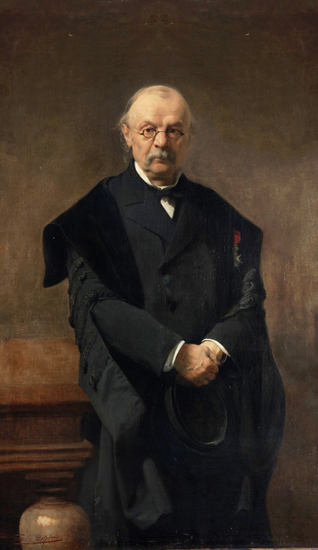
\small\textit{Eugène Charles Catalan (1814--1894)}\\[2pt]
\tiny Public domain, Émile Delperée, via Wikimedia Commons
\end{minipage}
\end{center}
```
:::
::: {.content-visible when-format="html"}
<div style="display:flex; align-items:center; margin:1em 0; gap:12px;">
<img src="images/Eugene_charles_catalan.jpg" style="width:100px; flex-shrink:0;" alt="Eugène Charles Catalan">
<div style="font-size:0.82em;"><em>Eugène Charles Catalan (1814–1894)</em><br><span style="font-size:0.85em;">Public domain, Émile Delperée, via Wikimedia Commons</span></div>
</div>
:::
**Example: the Catalan numbers.** A student counting the number
of ways to fully parenthesize a product of $n+1$ factors gets
1, 1, 2, 5, 14, 42, 132, ... A different student counting the
number of ways to triangulate a convex polygon with $n+2$ vertices
gets the same list. Entering "1, 1, 2, 5, 14, 42" in the OEIS
returns A000108 -- the Catalan numbers -- with over 200 distinct
combinatorial interpretations and dozens of references.
```{python}
import math

# Catalan numbers: C(n) = (2n choose n) / (n + 1)
# math.comb was introduced in @sec-pascal-binomial
catalan = [
    math.comb(2*n, n) // (n + 1)
    for n in range(12)
]
print(catalan)
```
Entering the first six of those values into oeis.org confirms they
are A000108. The OEIS entry then provides a recurrence
$C(n) = \frac{2(2n-1)}{n+1}\,C(n-1)$, a generating function, and
dozens of papers -- a complete research starter kit.
## Difference Tables {#sec-oeis-diff}
Given a sequence, how do you know whether $a(n)$ is a polynomial
in $n$? The answer comes from repeated *differences*.
Define the *forward difference operator* $\Delta$ by
$$\Delta a(n) = a(n+1) - a(n).$$
Applying $\Delta$ to consecutive terms builds one new (shorter) row.
Repeating the process builds a *difference table*. The key result:
> If $a(n)$ is a polynomial of degree $d$, the $d$-th row of
> differences is constant, and all later rows are zero.
For squares, the first differences are the odd numbers and the
second differences are all 2. This runs in reverse too: a sequence
whose second differences are all constant must come from a
quadratic formula.
```{python}
def diff_table(seq):
    rows = [list(seq)]
    while len(rows[-1]) > 1:
        r = rows[-1]
        rows.append(
            [r[i+1] - r[i] for i in range(len(r) - 1)]
        )
    return rows

# squares: a(n) = n^2
sq8 = [n**2 for n in range(1, 9)]
table = diff_table(sq8)
for i, row in enumerate(table):
    label = f"D{i}" if i > 0 else "  "
    vals = "  ".join(str(v).rjust(3) for v in row)
    print(f"{label}: {vals}")
```
D2 is constant (all 2s) and D3 is all zeros, confirming that $n^2$
is exactly degree 2. Now try the triangular numbers $T(n) = n(n+1)/2$:
```{python}
# uses: diff_table()

tri8 = [n*(n+1)//2 for n in range(1, 9)]
table2 = diff_table(tri8)
for i, row in enumerate(table2):
    label = f"D{i}" if i > 0 else "  "
    vals = "  ".join(str(v).rjust(3) for v in row)
    print(f"{label}: {vals}")
```
D1 is the natural numbers and D2 is all 1s -- the sequence is
degree 2, as expected from the formula $n(n+1)/2$. If differences
never stabilize, the sequence is not polynomial; no amount of
differencing will produce a constant row.
### Research Example: Does Differencing Always Flatten? {.unnumbered .unlisted}
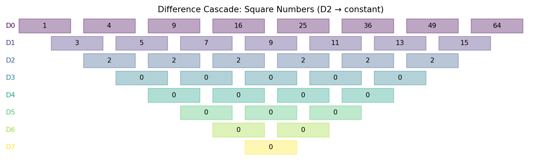
**Proposal.** The square numbers $a(n) = n^2$ come from a degree-2 polynomial. Can we *see* that degree directly — by repeatedly subtracting consecutive terms until a row goes constant — without knowing the formula in advance?
```{python}
#| label: fig-oeis-diffcascade
# uses: diff_table()
import matplotlib.pyplot as plt

def plot_diff_cascade(seq, title):
    rows = diff_table(seq)
    cmap = plt.get_cmap('viridis')
    n_rows = len(rows)
    fig, ax = plt.subplots(figsize=(9, 2.8))
    ax.set_xlim(-0.5, len(seq) - 0.5)
    ax.set_ylim(-0.5, n_rows - 0.5)
    ax.axis('off')
    for ri, row in enumerate(rows):
        color = cmap(ri / max(n_rows - 1, 1))
        offset = ri / 2.0
        for ci, val in enumerate(row):
            x = ci + offset
            y = n_rows - 1 - ri
            rect = plt.Rectangle(
                (x - 0.4, y - 0.4), 0.8, 0.8,
                color=color, alpha=0.35, zorder=1)
            ax.add_patch(rect)
            ax.text(x, y, str(val), ha='center', va='center',
                    fontsize=8, color='black', zorder=2)
        label = "D0" if ri == 0 else f"D{ri}"
        ax.text(-0.45, n_rows - 1 - ri, label,
                ha='right', va='center',
                fontsize=8, color=cmap(ri / max(n_rows - 1, 1)))
    ax.set_title(title, fontsize=10)
    plt.tight_layout()
    plt.show()

sq8 = [n**2 for n in range(1, 9)]
plot_diff_cascade(sq8, "Difference Cascade: Square Numbers (D2 → constant)")
```
D2 locks onto the constant 2 and D3 vanishes entirely — exactly what degree-2 predicts. You just *measured* the polynomial degree of a sequence using nothing but subtraction: no formula needed, no algebra required. Every polynomial hides its degree in its difference table like a fingerprint, and Python lets you see it in seconds.
## Identifying Recurrences {#sec-oeis-recurrence}
Many important sequences satisfy a *linear recurrence with constant
coefficients*:
$$a(n) = c_1\,a(n-1) + c_2\,a(n-2) + \cdots + c_k\,a(n-k).$$
Given enough terms, we can solve for the coefficients. For an
order-2 recurrence and known terms $a(0), a(1), a(2), a(3)$:
$$a(2) = c_1 \cdot a(1) + c_2 \cdot a(0)$$
$$a(3) = c_1 \cdot a(2) + c_2 \cdot a(1)$$
Two equations, two unknowns. SymPy's `solve` (introduced in
@sec-primes-what) handles this exactly with no floating-point error.
```{python}
from sympy import symbols, solve

def find_recurrence_2(seq):
    # find c1, c2 with a(n) = c1*a(n-1) + c2*a(n-2)
    c1, c2 = symbols('c1 c2')
    eq1 = c1*seq[1] + c2*seq[0] - seq[2]
    eq2 = c1*seq[2] + c2*seq[1] - seq[3]
    return solve([eq1, eq2], [c1, c2])

fib   = [1, 1, 2, 3, 5, 8, 13, 21]
lucas = [2, 1, 3, 4, 7, 11, 18, 29]

print("Fibonacci recurrence:", find_recurrence_2(fib))
print("Lucas recurrence:    ", find_recurrence_2(lucas))
```
Both sequences return $c_1 = 1, c_2 = 1$: both satisfy
$a(n) = a(n-1) + a(n-2)$, differing only in their starting values.
This is why Fibonacci and Lucas numbers share so many properties
(see @sec-fib-identities).
Once you have candidate coefficients, verify them on all remaining
terms to be sure the solution is not an accident of the first four
values:
```{python}
# uses: find_recurrence_2()

def verify_recurrence(seq, c1, c2):
    return all(
        seq[n] == c1*seq[n-1] + c2*seq[n-2]
        for n in range(2, len(seq))
    )

print(verify_recurrence(fib,   1, 1))
print(verify_recurrence(lucas, 1, 1))
```
If `find_recurrence_2` returns an empty dict, no order-2 linear
recurrence fits. Try order 3 by adding a third equation involving
$a(4)$ and a third unknown $c_3$, and so on. The Tribonacci numbers
$T(n) = T(n-1) + T(n-2) + T(n-3)$ require exactly this treatment.
## Recaman's Sequence {#sec-oeis-recaman}
::: {.content-visible when-format="pdf"}
```{=latex}
\begin{center}
\begin{minipage}[c]{0.28\textwidth}\centering
\href{https://youtu.be/FGC5TdIiT9U}{\includegraphics[width=\textwidth]{images/thumb_FGC5TdIiT9U.jpg}}
\end{minipage}%
\hspace{0.02\textwidth}%
\begin{minipage}[c]{0.28\textwidth}
\small\textbf{Numberphile}\\[3pt]
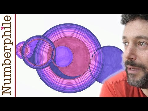
\small The Slightly Spooky Recamán Sequence\\[3pt]
\small\href{https://youtu.be/FGC5TdIiT9U}{\texttt{youtu.be/FGC5TdIiT9U}}
\end{minipage}%
\hspace{0.02\textwidth}%
\begin{minipage}[c]{0.36\textwidth}
\small A sequence that prefers going back but can't — the arcs it draws look accidental, yet nobody knows whether every positive integer eventually appears.
\end{minipage}
\end{center}
```
:::
::: {.content-visible when-format="html"}
<div style="display:flex; align-items:flex-start; margin:1em 0; gap:12px; width:100%;">
<div style="flex:0 0 200px;"><a href="https://youtu.be/FGC5TdIiT9U" target="_blank"><img src="https://img.youtube.com/vi/FGC5TdIiT9U/0.jpg" style="width:100%;" alt="The Slightly Spooky Recamán Sequence"></a></div>
<div style="flex:1; font-size:0.85em;"><strong>Numberphile</strong><br>The Slightly Spooky Recamán Sequence<br><a href="https://youtu.be/FGC5TdIiT9U" target="_blank" style="font-family:monospace;">youtu.be/FGC5TdIiT9U</a></div>
<div style="flex:1; font-size:0.85em;">A sequence that prefers going back but can't — the arcs it draws look accidental, yet nobody knows whether every positive integer eventually appears.</div>
</div>
:::
Some sequences are defined by a simple rule that hides a deep open
question. Recaman's sequence (OEIS A005132) is one of them.
**Rule.** Start with $a(0) = 0$. At each step $k$:
- *Subtract* $k$ from $a(k-1)$ if the result is positive and has
not yet appeared in the sequence.
- Otherwise, *add* $k$ to $a(k-1)$.
The first terms are 0, 1, 3, 6, 2, 7, 13, 20, 12, 21, 11, 22, 10, 23, 9, ...
The sequence prefers to go down, but must go up when a downward
step would revisit a value or land on zero. This creates the chaotic
bouncing trajectory that makes Recaman's sequence visually striking.
To check membership efficiently, Python's `set` is ideal. A `set`
stores unique values and supports `x in seen` in constant time --
no matter how large `seen` grows. A list scan would take time
proportional to the list's length; for long sequences that
difference is enormous.
```{python}
import pprint

def recaman(n):
    a = [0] * n
    seen = {0}          # set: O(1) membership check
    for k in range(1, n):
        candidate = a[k-1] - k
        if candidate > 0 and candidate not in seen:
            a[k] = candidate
        else:
            a[k] = a[k-1] + k
        seen.add(a[k])
    return a

seq30 = recaman(30)
# width=60 wraps long output to fit the printed page
pprint.pprint(seq30, width=60, compact=True)
```
The open question: does every positive integer eventually appear in
Recaman's sequence? After computing tens of billions of terms, no
one has found a missing integer -- but no proof exists either.
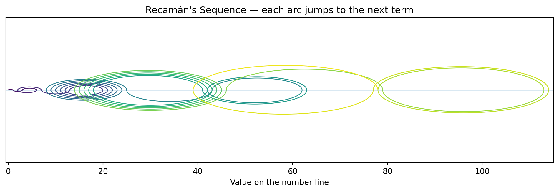
### Research Example: What Does Recamán's Sequence Look Like? {.unnumbered .unlisted}
**Proposal.** Recamán's sequence prefers to go left but cannot always — it must jump right when a leftward step would revisit a number. Draw each step as a semicircle on the number line, alternating above and below. What does 40 steps of this back-and-forth look like?
```{python}
#| label: fig-oeis-recaman
# uses: recaman()
import matplotlib.pyplot as plt
import matplotlib.patches as mpatches

BLUE = '#1f77b4'

seq = recaman(40)
fig, ax = plt.subplots(figsize=(10, 3.5))
cmap = plt.get_cmap('viridis')
maxv = max(seq)
for k in range(1, len(seq)):
    x1, x2 = seq[k-1], seq[k]
    cx = (x1 + x2) / 2.0
    r = abs(x2 - x1) / 2.0
    color = cmap(k / len(seq))
    theta1, theta2 = (0, 180) if k % 2 == 1 else (180, 360)
    arc = mpatches.Arc((cx, 0), 2*r, 2*r,
                       angle=0, theta1=theta1, theta2=theta2,
                       color=color, lw=1.0)
    ax.add_patch(arc)
ax.axhline(0, color=BLUE, lw=0.5)
ax.set_xlim(-0.5, maxv + 1)
ax.set_ylim(-maxv / 2, maxv / 2)
ax.set_yticks([])
ax.set_xlabel("Value on the number line")
ax.set_title("Recamán's Sequence — each arc jumps to the next term")
plt.tight_layout()
plt.show()
```
Each arc sweeps from one term to the next along the number line, alternating above and below. The sequence prefers to arc left (subtract), but arcs right (add) whenever a leftward jump would revisit territory already claimed. The arcs look almost organic — yet this entire picture emerges from a rule short enough to fit on a sticky note. Nobody has proved whether every integer eventually appears; your computer just drew the open question.
## The Look-and-Say Sequence {#sec-oeis-look-say}
::: {.content-visible when-format="pdf"}
```{=latex}
\begin{center}
\begin{minipage}[c]{0.22\textwidth}
\includegraphics[width=\textwidth]{images/Conway_dmv_1987_berlin.jpg}
\end{minipage}%
\hspace{0.03\textwidth}%
\begin{minipage}[c]{0.55\textwidth}
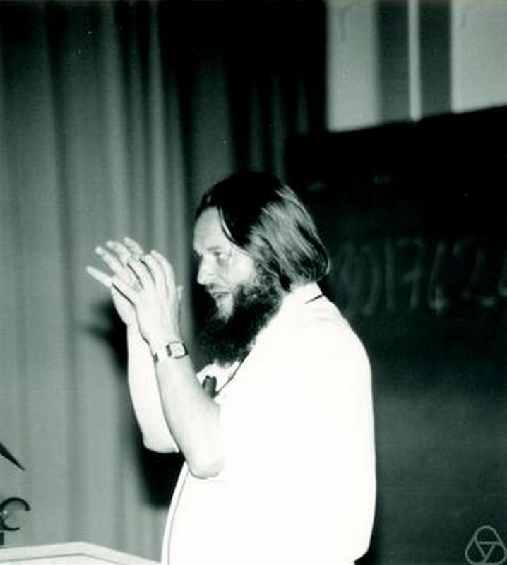
\small\textit{John Horton Conway (1937--2020)}\\[2pt]
\tiny CC BY-SA 2.0 de, Konrad Jacobs, via Wikimedia Commons
\end{minipage}
\end{center}
```
:::
::: {.content-visible when-format="html"}
<div style="display:flex; align-items:center; margin:1em 0; gap:12px;">
<img src="images/Conway_dmv_1987_berlin.jpg" style="width:100px; flex-shrink:0;" alt="John Horton Conway">
<div style="font-size:0.82em;"><em>John Horton Conway (1937–2020)</em><br><span style="font-size:0.85em;">CC BY-SA 2.0 de, Konrad Jacobs, via Wikimedia Commons</span></div>
</div>
:::
Start with the string "1". Read it aloud, then write down what you
said. "One one" becomes "11". Read that aloud: "two ones" becomes
"21". Continue: "one two, one one" becomes "1211". The sequence
of strings starts:
| Generation | String |
|:----------:|:--------:|
| 1 | 1 |
| 2 | 11 |
| 3 | 21 |
| 4 | 1211 |
| 5 | 111221 |
| 6 | 312211 |
This is OEIS A005150. The generating rule: scan the current string
from left to right, group consecutive identical digits, and replace
each group with its count followed by the digit.
```{python}
def look_and_say(s):
    result = ""
    i = 0
    while i < len(s):
        c = s[i]
        count = 0
        while i < len(s) and s[i] == c:
            count += 1
            i += 1
        result += str(count) + c
    return result

# uses: look_and_say()

gen = "1"
for step in range(1, 7):
    print(f"Gen {step}: {gen}")
    gen = look_and_say(gen)
```
::: {.content-visible when-format="pdf"}
```{=latex}
\begin{center}
\begin{minipage}[c]{0.28\textwidth}\centering
\href{https://youtu.be/ea7lJkEhytA}{\includegraphics[width=\textwidth]{images/thumb_ea7lJkEhytA.jpg}}
\end{minipage}%
\hspace{0.02\textwidth}%
\begin{minipage}[c]{0.28\textwidth}
\small\textbf{Numberphile}\\[3pt]
\small Look-and-Say Numbers (feat.\ John Conway)\\[3pt]
\small\href{https://youtu.be/ea7lJkEhytA}{\texttt{youtu.be/ea7lJkEhytA}}
\end{minipage}%
\hspace{0.02\textwidth}%
\begin{minipage}[c]{0.36\textwidth}
\small John Conway explains his 1986 discovery: the look-and-say sequence grows by a factor of $\approx 1.3036$ per generation, governed by 92 atomic sub-sequences.
\end{minipage}
\end{center}
```
:::
::: {.content-visible when-format="html"}
<div style="display:flex; align-items:flex-start; margin:1em 0; gap:12px; width:100%;">
<div style="flex:0 0 200px;"><a href="https://youtu.be/ea7lJkEhytA" target="_blank"><img src="https://img.youtube.com/vi/ea7lJkEhytA/0.jpg" style="width:100%;" alt="Look-and-Say Numbers (feat John Conway)"></a></div>
<div style="flex:1; font-size:0.85em;"><strong>Numberphile</strong><br>Look-and-Say Numbers (feat. John Conway)<br><a href="https://youtu.be/ea7lJkEhytA" target="_blank" style="font-family:monospace;">youtu.be/ea7lJkEhytA</a></div>
<div style="flex:1; font-size:0.85em;">John Conway explains his 1986 discovery: the look-and-say sequence grows by a factor of ≈ 1.3036 per generation, governed by 92 atomic sub-sequences.</div>
</div>
:::
The string grows with each step. Strikingly, the growth rate
converges to a constant. In 1986, John Conway proved that the
length of each generation is approximately 1.303577 times the
length of the previous one [@conway1986].
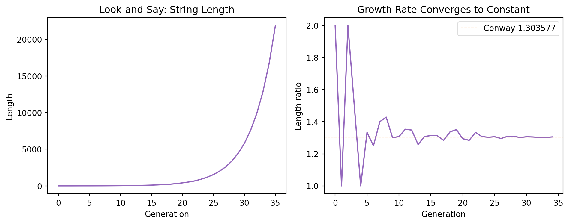
### Research Example: Does Look-and-Say Grow at a Constant Rate? {.unnumbered .unlisted}
**Proposal.** Each generation of look-and-say is longer than the last — but is the growth rate predictable? Conway claimed the ratio of consecutive lengths converges to a specific constant near 1.3036. Plot 35 generations of string length and watch the ratio lock onto its target.
```{python}
#| label: fig-oeis-looksay
# uses: look_and_say()
import matplotlib.pyplot as plt

PURPLE = '#9467bd'
ORANGE = '#ff7f0e'

gen = "1"
lengths = [len(gen)]
for _ in range(35):
    gen = look_and_say(gen)
    lengths.append(len(gen))

ratios = [lengths[k] / lengths[k-1]
          for k in range(1, len(lengths))]

fig, axes = plt.subplots(1, 2, figsize=(10, 4))
axes[0].plot(lengths, color=PURPLE)
axes[0].set_xlabel("Generation")
axes[0].set_ylabel("Length")
axes[0].set_title("Look-and-Say: String Length")
axes[1].plot(ratios, color=PURPLE)
axes[1].axhline(1.303577, color=ORANGE, lw=0.8,
                linestyle="--", label="Conway 1.303577")
axes[1].set_xlabel("Generation")
axes[1].set_ylabel("Length ratio")
axes[1].set_title("Growth Rate Converges to Constant")
axes[1].legend()
plt.tight_layout()
plt.show()
```
By generation 30 the ratio has settled to five decimal places — the curve kisses the orange dashed line and stays there. You just confirmed, computationally, a theorem that took Conway years of analysis. A word game obeying a precise exponential growth law is exactly the kind of surprise that makes mathematical research addictive.
Conway also proved that starting from any seed (except "22"), the
look-and-say sequence eventually decomposes into a fixed collection
of 92 independent sub-strings he called *chemical elements*. The
constant 1.303577... is the largest real root of a polynomial of
degree 71 -- exact mathematics hiding inside a word game.
## Using the OEIS as a Research Tool {#sec-oeis-tool}
The most useful skill this chapter can teach is the full workflow:
from a counting problem to a sequence to an OEIS entry to a set of
open questions. Here it is in one worked example.
**Step 1: pose a counting problem.** How many ways can you climb
$n$ stairs by taking steps of 1 or 2 at a time? For $n = 3$ the
options are 1+1+1, 1+2, and 2+1 -- three ways.
**Step 2: write code to generate terms.**
```{python}
def stair_count(n):
    # ways to climb n stairs in steps of 1 or 2
    if n == 0:
        return 1
    ways = [1, 1]
    for k in range(2, n + 1):
        ways.append(ways[-1] + ways[-2])
    return ways[n]

# uses: stair_count()

seq = [stair_count(n) for n in range(1, 14)]
print(seq)
```
**Step 3: recognize or look up the sequence.** The output is
1, 2, 3, 5, 8, 13, 21, 34, 55, 89, 144, 233, 377. That is the
Fibonacci sequence shifted by one position: $\text{stair\_count}(n) = F(n+1)$.
Entering "1, 2, 3, 5, 8, 13, 21" into oeis.org returns A000045
and confirms the connection.
**Step 4: read the OEIS entry.** A000045 lists hundreds of
combinatorial interpretations, related sequences (A001654 is
products of consecutive Fibonacci numbers; A007970 is Fibonacci
numbers that are also perfect squares), and links to dozens of
open problems. Each is a potential research direction.
**Step 5: vary the problem.** What if steps can be 1, 2, or 3?
The resulting sequence is the Tribonacci numbers (OEIS A000073).
What if the staircase has $m$ steps but wraps around in a circle?
That question connects to Pisano periods (see @sec-fib-pisano).
What if the allowed step sizes change -- say 1, 3, and 5 only?
That is a new sequence; if the OEIS does not list it, you may have
found something worth submitting.
The OEIS is most valuable when your computed sequence *matches
something you did not expect*. That surprise -- your counting
problem turns out to be a 100-year-old sequence -- is where
experimental mathematical research begins.
## Further Research Topics {#sec-oeis-research}
1. Compute the difference table of the cube numbers $a(n) = n^3$
for $n = 1, 2, \ldots, 8$. At which level do the differences
become constant, and what is that constant? Use the fact that
the leading coefficient of a degree-$d$ polynomial determines
the constant in the $d$-th difference row to predict the answer
before computing it. *(Problem proposed by Claude Code.)*
2. The triangular numbers $T(n) = n(n+1)/2$ satisfy the simple
recurrence $T(n) = T(n-1) + n$, which is not a constant-coefficient
recurrence. Apply `find_recurrence_2` to the first eight
triangular numbers. Does it return a solution? What does the
answer (or non-answer) tell you about the sequence? *(Problem proposed by Claude Code.)*
3. The Padovan sequence is defined by $P(0) = P(1) = P(2) = 1$ and
$P(n) = P(n-2) + P(n-3)$. Generate the first 25 terms and look
up the sequence in the OEIS. The ratio $P(n)/P(n-1)$ converges
to the *plastic constant* $\rho \approx 1.3247$. Track this
convergence computationally and compare its speed to the golden
ratio convergence in the Fibonacci sequence (see @sec-fib-golden). *(Problem proposed by Claude Code.)*
4. Extend `find_recurrence_2` to find order-3 recurrences by setting
up a $3 \times 3$ linear system using $a(2), a(3), a(4)$ and
solving for $c_1, c_2, c_3$. Use it to discover the recurrence
for the Tribonacci numbers: 0, 0, 1, 1, 2, 4, 7, 13, 24, 44, ...
Verify that order 2 fails and order 3 succeeds. *(Problem proposed by Claude Code.)*
5. Write a function that checks whether every integer from 1 to $N$
appears in the first $M$ terms of Recaman's sequence. For $N = 50$,
find the smallest $M$ such that all integers up to 50 are covered.
Plot the smallest such $M$ as a function of $N$ for $N = 10, 20,
\ldots, 200$. Does $M$ grow linearly, quadratically, or faster? *(Problem proposed by Claude Code.)*
6. The Van Eck sequence is defined by $a(0) = 0$; for $n \ge 1$,
$a(n)$ equals how many steps back $a(n-1)$ last appeared, or 0
if $a(n-1)$ has not appeared before. Generate the first 300 terms
and plot them. The conjecture that every non-negative integer
eventually appears remains open. *(Problem proposed by Claude Code.)*
7. Conway proved that every look-and-say sequence eventually
consists of 92 independent "elements" [@conway1986] (except seeds containing
the digit 2 in isolation). Starting from "1", apply `look_and_say`
30 times and search the resulting string for the sub-string "22".
How many times does it appear? Does starting from "3" change the
behavior? *(Problem proposed by Claude Code.)*
8. The Stern diatomic sequence is defined by $s(0) = 0$, $s(1) = 1$,
$s(2n) = s(n)$, $s(2n+1) = s(n) + s(n+1)$. Generate the first
128 terms. The claim: every positive rational $p/q$ (in lowest
terms) appears exactly once as $s(n+1)/s(n)$ for some $n$ [@stern1858].
Verify this computationally for all rationals with $p + q \le 15$.
(Use `fractions.Fraction` from @sec-cfrac-convergents to handle
exact reduction.) *(Problem proposed by Claude Code.)*
9. The Golomb self-describing sequence $G$ satisfies: $G(1) = 1$,
and the value $k$ appears exactly $G(k)$ times in $G$. Generate
the first 60 terms by building the sequence greedily. The
asymptotic formula $G(n) \sim \phi^{2-\phi}\, n^{\phi-1}$
(where $\phi$ is the golden ratio, see @sec-fib-golden) was
proved by Golomb himself [@golomb1965]. Test its accuracy at $n = 20, 40, 60$. *(Problem proposed by Claude Code.)*
10. Hofstadter's $Q$-sequence is $Q(1) = Q(2) = 1$ and
$Q(n) = Q(n - Q(n-1)) + Q(n - Q(n-2))$. Generate as many
terms as possible and plot $Q(n)/n$. The ratio fluctuates
chaotically near $1/2$. Count how often $Q(n)/n < 0.45$ in
the first 5,000 terms, and whether the fraction of such $n$
is increasing or decreasing as $n$ grows. *(Problem proposed by Claude Code.)*
11. A sequence is called *self-describing* if $a(n)$ gives the
number of times $n$ appears as a value in the entire sequence.
There is exactly one such sequence that begins $a(1) = 1$,
$a(2) = 2$, $a(3) = 1$, ... Find it by building it greedily:
the constraints force each term one by one. Look up the result
in the OEIS. *(Problem proposed by Claude Code.)*
12. Build a mini-OEIS: a Python dictionary whose keys are strings
like "A000045" and whose values are lists of the first 20 terms.
Populate it with at least 12 sequences from this book (primes,
Fibonacci, Lucas, Catalan, Recaman, and others). Write a search
function: given a list of five terms, return all A-numbers whose
stored sequence contains those five consecutive terms. What is
the minimum prefix length needed to distinguish each stored
sequence from all others? *(Problem proposed by Claude Code.)*
13. Ulam's lucky numbers: start with all positive integers, remove
every second one (leaving the odd numbers), note the second
remaining is 3 -- remove every third remaining number, then
every fifth (the new second survivor), and so on. Generate the
first 100 lucky numbers. The prime number theorem gives
$\pi(n) \approx n / \ln n$; a similar "lucky number theorem"
conjectures the same asymptotic for the lucky number count.
Test this conjecture computationally up to $n = 1000$. *(Problem proposed by Claude Code.)*
14. The Motzkin numbers $M(n)$ count lattice paths from $(0,0)$ to
$(n,0)$ using unit steps right-up, right, and right-down that
never go below the $x$-axis. They satisfy
$(n+2)\,M(n) = (2n+2)\,M(n-1) + 3\,M(n-2)$ with $M(0) = M(1) = 1$.
Generate the first 20 terms and verify them against OEIS A001006.
Compare the growth rate of Motzkin numbers to Catalan numbers
by plotting the ratio $M(n)/C(n)$ for $n = 1, \ldots, 20$. *(Problem proposed by Claude Code.)*
15. Conway's look-and-say sequence starting from "1" eventually
breaks into 92 atomic sub-strings ("chemical elements") [@conway1986] that
evolve independently. After 30 generations the string is
thousands of characters long. Split it by scanning for the
known boundary marker string "22" preceded and followed by
non-2 digits, and count how many distinct element sub-strings
appear. Do the 10 most common elements account for more than
half the total length? *(Problem proposed by Claude Code.)*
16. Consider the recurrence $a(1) = 7$, $a(n) = a(n-1) +
\gcd(n,\, a(n-1))$. Compute $g(n) = a(n) - a(n-1)$ for
$n = 2, 3, \ldots, 200$. Every $g(n)$ equals either 1 or a
prime — a fact proved by E. Rowland [@rowland2008jis]. Confirm
this computationally: collect all $g(n) > 1$ and check each for
primality using trial division (see @sec-primes-sieve). Observe
that the prime 2 never appears among the differences, and that 3
dominates: roughly half the non-trivial differences equal 3.
What other primes appear in the first 400 differences, and how
often does each occur? Change the starting value from 7 to 11,
then to 17. Does the pattern — every difference is 1 or prime —
persist for other starting values? OEIS A106108 documents the
primes generated by Rowland's sequence; look up what is known
about which primes can appear. *(Problem proposed by Claude Code.)*
17. The *partition function* $p(n)$ counts the number of ways to
write $n$ as an unordered sum of positive integers: for instance
$p(4) = 5$ because $4 = 3+1 = 2+2 = 2+1+1 = 1+1+1+1$ along with
$4$ itself. Compute $p(n)$ for $n = 0, 1, \ldots, 60$ using a
dynamic-programming table (start with `dp[0] = 1` and update
`dp[j] += dp[j-k]` for each $k$). Then verify Ramanujan's
congruence [@ramanujan1919congruences]:
$$p(5k + 4) \equiv 0 \pmod{5} \quad \text{for all } k \geq 0.$$
You should find $p(4) = 5$, $p(9) = 30$, $p(14) = 135$, all
divisible by 5. Two companion congruences — $p(7k+5) \equiv 0
\pmod 7$ and $p(11k+6) \equiv 0 \pmod{11}$ — also hold.
Verify both for $k = 0, 1, \ldots, 5$. As a further challenge,
compute $p(n) \bmod 2$ for $n = 0, \ldots, 100$ and describe the
pattern visually; the question of which $n$ give $p(n)$ odd is
still not fully resolved. *(Problem proposed by Claude Code.)*
18. The *EKG sequence* (OEIS A064413) is built greedily: $a(1)=1$,
$a(2)=2$, and for each subsequent position $a(n)$ is the
*smallest unused positive integer* sharing a common factor
greater than 1 with $a(n-1)$. Implement this with a `set` to
track used values (see the Recaman code in this chapter for the
same pattern). Generate the first 100 terms; the sequence begins
1, 2, 4, 6, 3, 9, 12, 8, 10, 5, 15, 18, 14, 7, 21, \ldots\
It was proved [@lagarias2002ekg] that this is a *permutation* of
all positive integers — every integer appears exactly once.
Verify no value repeats in your first 200 terms. Plot the
sequence; the jagged up-down pattern resembles an
electrocardiogram, which is how the sequence got its name.
Identify where each prime $p \leq 29$ first appears and tabulate
the positions. Notice that primes are always sandwiched between
runs of even numbers. Can you predict, for a given prime $p$,
roughly where it will appear? *(Problem proposed by Claude Code.)*
19. Define the *Somos-4* recurrence by the rule
$a(n)\,a(n-4) = a(n-1)\,a(n-3) + a(n-2)^2$
starting from $a(1)=a(2)=a(3)=a(4)=1$. Use
`fractions.Fraction` (see @sec-cfrac-convergents) so that
every arithmetic step is exact. Compute 20 terms; you should get
1, 1, 1, 1, 2, 3, 7, 23, 59, 314, \ldots, all integers, even
though the rule divides at every step. This is an instance of the
*Laurent phenomenon* [@fomin2002laurent]: the solution, expressed
in terms of the initial values, is always a Laurent polynomial
with integer coefficients. Now try the *Somos-8* recurrence
$a(n)\,a(n-8) = a(n-1)\,a(n-7)+a(n-2)\,a(n-6)+a(n-3)\,a(n-5)+a(n-4)^2$
with eight initial 1s. Compute 20 terms and find that term 18
equals $420514/7$ — integrality has failed. The Laurent
phenomenon covers Somos-4 through Somos-7 but not Somos-8.
Verify that Somos-5, Somos-6, and Somos-7 (write down their
recurrences from the pattern) also stay integer for the first 30
terms, then confirm Somos-8 breaks. *(Problem proposed by Claude Code.)*
20. The *Thue-Morse sequence* $t(n)$ is defined by $t(n) = 1$ if
the number of 1-bits in the binary representation of $n$ is odd,
and $t(n) = 0$ otherwise: so $t(0)=0,\, t(1)=1,\, t(2)=1,\,
t(3)=0,\ldots$ (use `bin(n).count('1') % 2` in Python). Partition
the integers $\{0, 1, \ldots, 15\}$ into the set $S_0$ where
$t(n)=0$ and the set $S_1$ where $t(n)=1$. Compute $\sum_{x \in
S_0} x^k$ and $\sum_{x \in S_1} x^k$ for $k = 1, 2, 3$; the two
sums are equal in every case. This is the *Prouhet–Tarry–Escott
property* [@allouche2003automatic]: the Thue-Morse partition of
$\{0,\ldots, 2^n - 1\}$ yields two sets with equal sums of
$k$-th powers for $k = 0, 1, \ldots, n-1$. Verify it for $n=4$
(the set $\{0,\ldots,15\}$, testing $k = 1,2,3$) and for $n=5$
(the set $\{0,\ldots,31\}$, testing $k=1,2,3,4$). Write a
general function `check_pte(n)` that builds $S_0$, $S_1$, and
verifies equality for all $k < n$. The PTE problem — finding
*small* sets with equal power sums — is an open combinatorics
problem; the Thue-Morse construction gives one infinite family of
solutions. *(Problem proposed by Claude Code.)*