# Pascal's Triangle: Arithmetic in a Grid {#sec-pascal}
```{python}
#| echo: false
from pathlib import Path; import urllib.request
_d = Path('images'); _d.mkdir(exist_ok=True)
_p = _d / 'Blaise_Pascal_Versailles-cropped.jpg'
if not _p.exists():
try: urllib.request.urlretrieve(
'https://upload.wikimedia.org/wikipedia/commons/9/98/Blaise_Pascal_Versailles.JPG', _p)
except Exception: pass
```
::: {.content-visible when-format="pdf"}
```{=latex}
\begin{center}
\begin{minipage}[c]{0.22\textwidth}
\includegraphics[width=\textwidth]{images/Blaise_Pascal_Versailles-cropped.jpg}
\end{minipage}%
\hspace{0.03\textwidth}%
\begin{minipage}[c]{0.55\textwidth}
\small\textit{Blaise Pascal (1623--1662)}\\[2pt]
\tiny CC BY 3.0, Philippe de Champaigne, via Wikimedia Commons
\end{minipage}
\end{center}
```
:::
::: {.content-visible when-format="html"}
<div style="display:flex; align-items:center; margin:1em 0; gap:12px;">
<img src="images/Blaise_Pascal_Versailles-cropped.jpg" style="width:100px; flex-shrink:0;" alt="Blaise Pascal">
<div style="font-size:0.82em;"><em>Blaise Pascal (1623–1662)</em><br><span style="font-size:0.85em;">CC BY 3.0, Philippe de Champaigne, via Wikimedia Commons</span></div>
</div>
:::
::: {.content-visible when-format="pdf"}
```{=latex}
\begin{center}
\begin{minipage}[c]{0.28\textwidth}
\centering
\href{https://youtu.be/XMriWTvPXHI}{\includegraphics[width=\textwidth]{images/thumb_XMriWTvPXHI.jpg}}
\end{minipage}%
\hspace{0.02\textwidth}%
\begin{minipage}[c]{0.28\textwidth}
\small\textbf{TED-Ed}\\[3pt]
\small The mathematical secrets of Pascal's triangle\\[3pt]
\small\href{https://youtu.be/XMriWTvPXHI}{\texttt{youtu.be/XMriWTvPXHI}}
\end{minipage}%
\hspace{0.02\textwidth}%
\begin{minipage}[c]{0.36\textwidth}
\small Uncovers the hidden patterns inside Pascal's triangle — Fibonacci numbers, powers of 2, and the Sierpiński fractal — all encoded in a simple grid of binomial coefficients.
\end{minipage}
\end{center}
```
:::
::: {.content-visible when-format="html"}
<div style="display:flex; align-items:flex-start; margin:1em 0; gap:12px; width:100%;">
<div style="flex:0 0 200px;"><a href="https://youtu.be/XMriWTvPXHI" target="_blank"><img src="https://img.youtube.com/vi/XMriWTvPXHI/0.jpg" style="width:100%;display:block;" alt="The mathematical secrets of Pascal's triangle"></a></div>
<div style="flex:1; font-size:0.85em;"><strong>TED-Ed</strong><br>The mathematical secrets of Pascal's triangle<br><a href="https://youtu.be/XMriWTvPXHI" target="_blank" style="font-family:Consolas,monospace;">youtu.be/XMriWTvPXHI</a></div>
<div style="flex:1; font-size:0.85em;">Uncovers the hidden patterns inside Pascal's triangle — Fibonacci numbers, powers of 2, and the Sierpiński fractal — all encoded in a simple grid of binomial coefficients.</div>
</div>
:::
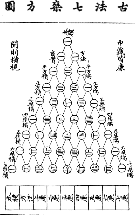
A medieval Chinese mathematician named Yang Hui recorded a triangular
arrangement of numbers in 1261. Blaise Pascal rediscovered and
popularized it in Europe four centuries later, and it now bears his
name. Every number in the triangle is the sum of the two above it, yet
buried inside this simple rule are the keys to probability,
combinatorics, and fractal geometry — and a secret about prime numbers
that eluded mathematicians for centuries. No other arrangement this
simple rewards curiosity so generously. Computation makes those keys
visible in ways that pen and paper cannot.
## Building the Triangle {#sec-pascal-build}
```{python}
#| echo: false
from pathlib import Path; import urllib.request
_d = Path('images'); _d.mkdir(exist_ok=True)
_p = _d / 'Yanghui_triangle.PNG'
if not _p.exists():
try: urllib.request.urlretrieve(
'https://upload.wikimedia.org/wikipedia/commons/2/26/Yanghui_triangle.PNG', _p)
except Exception: pass
```
::: {.content-visible when-format="pdf"}
```{=latex}
\begin{center}
\begin{minipage}[c]{0.28\textwidth}
\includegraphics[width=\textwidth]{images/Yanghui_triangle.PNG}
\end{minipage}%
\hspace{0.03\textwidth}%
\begin{minipage}[c]{0.48\textwidth}
\small\textit{Yang Hui's triangle, from a 1303 Chinese woodblock print.}\\[4pt]
\tiny Known in China centuries before Pascal.
Public domain, via Wikimedia Commons.
\end{minipage}
\end{center}
```
:::
::: {.content-visible when-format="html"}
<div style="display:flex; align-items:center; margin:1em 0; gap:12px;">
<img src="images/Yanghui_triangle.PNG" style="width:140px; flex-shrink:0;" alt="Yang Hui triangle woodblock print">
<div style="font-size:0.82em;"><em>Yang Hui's triangle, from a 1303 Chinese woodblock print.</em><br><span style="font-size:0.85em;">Known in China centuries before Pascal. Public domain, via Wikimedia Commons.</span></div>
</div>
:::
Label each position by its row $n$ (starting at 0) and its column $k$
(starting at 0). The triangle obeys a single rule:
$$C(n,\, k) = C(n-1,\, k-1) + C(n-1,\, k), \quad C(n,\, 0) = C(n,\, n) = 1.$$
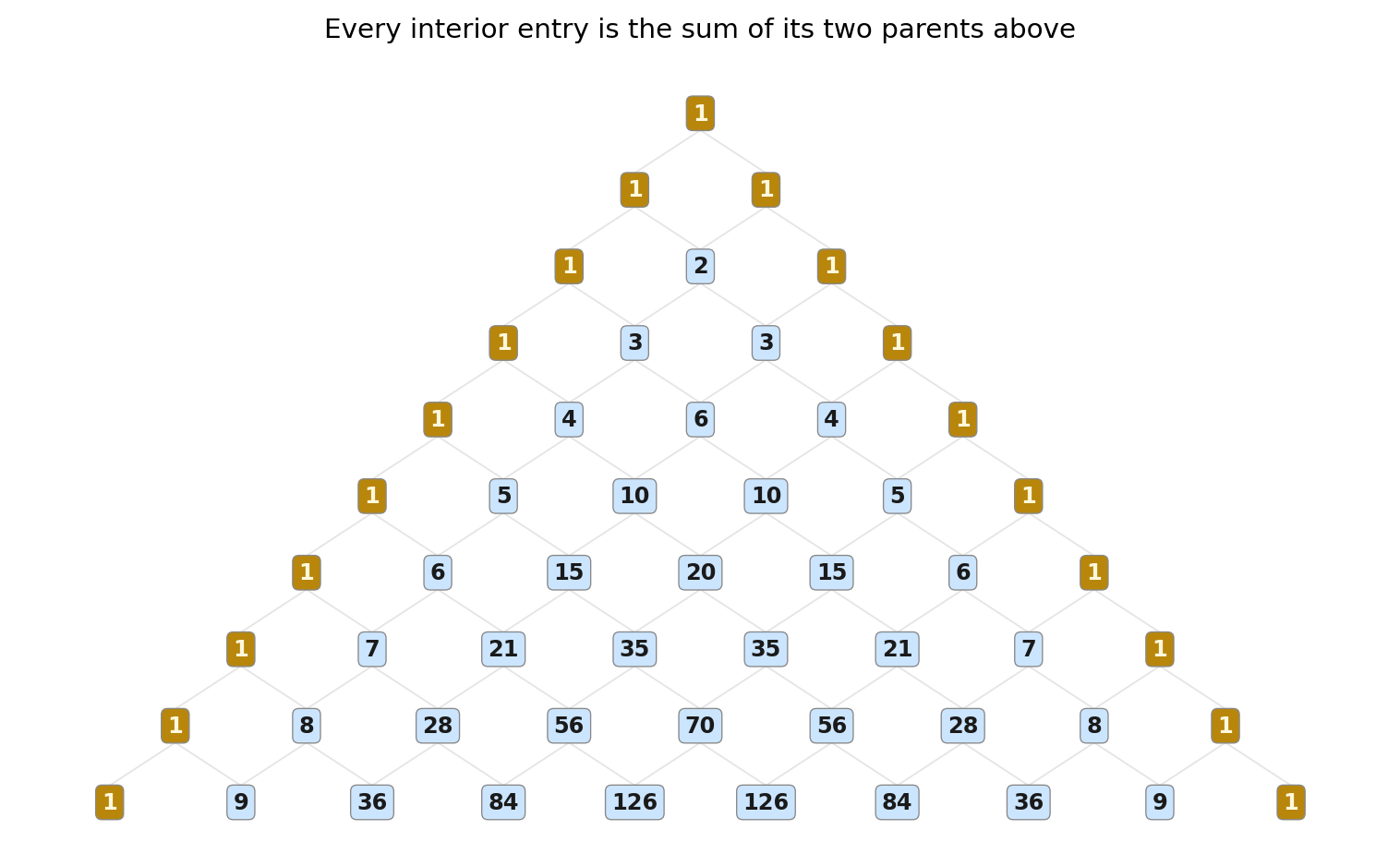
Every row begins and ends with 1; every interior entry is the sum of
its two parents.
```{python}
def pascal(rows):
    tri = [[1]]
    for n in range(1, rows):
        prev = tri[-1]
        new = [1]
        for k in range(n - 1):
            new.append(prev[k] + prev[k + 1])
        new.append(1)
        tri.append(new)
    return tri

tri = pascal(10)
for n, row in enumerate(tri):
    print(f"row {n}: {row}")
```
Row $n$ has exactly $n + 1$ entries. Notice how each interior number
is the sum of the pair above it: 3 = 1 + 2, 10 = 4 + 6, and so on.
The figure below draws the same triangle with its parent lines.
### Research Example: What Does Pascal's Triangle Actually Look Like? {.unnumbered .unlisted}
Draw the first 10 rows as a connected grid — does one addition rule produce a recognizable structure?
```{=latex}
\needspace{26\baselineskip}
```
```{python}
#| label: fig-pascal-build
#| fig-cap: "Pascal's Triangle: gold entries are the edge 1s; blue entries are sums of the two above."
import matplotlib.pyplot as plt

def pascal(rows):
    tri = [[1]]
    for n in range(1, rows):
        prev = tri[-1]
        new = [1]
        for k in range(n - 1):
            new.append(prev[k] + prev[k + 1])
        new.append(1)
        tri.append(new)
    return tri

tri = pascal(10)
N = len(tri)

fig, ax = plt.subplots(figsize=(8, 5))

for n, row in enumerate(tri):
    for k, val in enumerate(row):
        x = k - n / 2.0
        y = float(N - 1 - n)
        edge = (k == 0 or k == n)
        fc = '#b8860b' if edge else '#cce5ff'
        tc = '#fff8dc' if edge else '#1a1a1a'
        ax.text(x, y, str(val), ha='center', va='center',
                fontsize=9, color=tc, fontweight='bold',
                bbox=dict(boxstyle='round,pad=0.28', facecolor=fc,
                          edgecolor='#888888', linewidth=0.5))

for n in range(1, N):
    for k in range(n + 1):
        xc = k - n / 2.0
        yc = float(N - 1 - n)
        if k > 0:
            ax.plot([(k - 1) - (n - 1) / 2.0, xc],
                    [float(N - n) - 0.22, yc + 0.22],
                    color='#cccccc', lw=0.7, alpha=0.5)
        if k < n:
            ax.plot([k - (n - 1) / 2.0, xc],
                    [float(N - n) - 0.22, yc + 0.22],
                    color='#cccccc', lw=0.7, alpha=0.5)

ax.set_xlim(-5.2, 5.2)
ax.set_ylim(-0.6, N - 0.2)
ax.axis('off')
ax.set_title("Every interior entry is the sum of its two parents above",
             fontsize=11, pad=6)
plt.tight_layout()
plt.show()
```
One rule — sum the two above — assembles the entire triangle. Every number sits exactly where the recurrence demands it.
## Binomial Coefficients {#sec-pascal-binomial}
::: {.content-visible when-format="pdf"}
```{=latex}
\begin{center}
\begin{minipage}[c]{0.28\textwidth}\centering
\href{https://youtu.be/6YzrVUVO9M0}{\includegraphics[width=\textwidth]{images/thumb_6YzrVUVO9M0.jpg}}
\end{minipage}%
\hspace{0.02\textwidth}%
\begin{minipage}[c]{0.28\textwidth}
\small\textbf{Primer}\\[3pt]
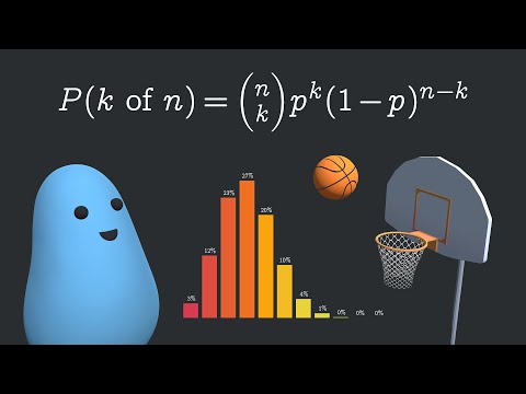
\small Overexplaining the Binomial Distribution\\[3pt]
\small\href{https://youtu.be/6YzrVUVO9M0}{\texttt{youtu.be/6YzrVUVO9M0}}
\end{minipage}%
\hspace{0.02\textwidth}%
\begin{minipage}[c]{0.36\textwidth}
\small Animated breakdown of why Pascal's triangle entries count the number of ways to choose $k$ items from $n$ — the combinatorial heart of every binomial expansion.
\end{minipage}
\end{center}
```
:::
::: {.content-visible when-format="html"}
<div style="display:flex; align-items:flex-start; margin:1em 0; gap:12px; width:100%;">
<div style="flex:0 0 200px;"><a href="https://youtu.be/6YzrVUVO9M0" target="_blank"><img src="https://img.youtube.com/vi/6YzrVUVO9M0/0.jpg" style="width:100%;" alt="Overexplaining the Binomial Distribution"></a></div>
<div style="flex:1; font-size:0.85em;"><strong>Primer</strong><br>Overexplaining the Binomial Distribution<br><a href="https://youtu.be/6YzrVUVO9M0" target="_blank" style="font-family:monospace;">youtu.be/6YzrVUVO9M0</a></div>
<div style="flex:1; font-size:0.85em;">Animated breakdown of why Pascal's triangle entries count the number of ways to choose k items from n — the combinatorial heart of every binomial expansion.</div>
</div>
:::
The entry at position $(n, k)$ counts the number of ways to choose
$k$ items from a collection of $n$ distinct items. This number is
called the **binomial coefficient** and is written $\binom{n}{k}$
("$n$ choose $k$"):
$$\binom{n}{k} = \frac{n!}{k!\,(n-k)!}.$$
For example, $\binom{5}{2} = 10$: from five books you can pick any
pair in ten different ways. Python's `math.comb` computes this
directly:
```{python}
import math

print(math.comb(10, 3))   # 120 ways to choose 3 from 10
print(math.comb(10, 7))   # same: choosing 7 is like leaving 3
```
The symmetry $\binom{n}{k} = \binom{n}{n-k}$ makes sense
combinatorially: choosing $k$ items to include is identical to
choosing $n - k$ items to exclude.
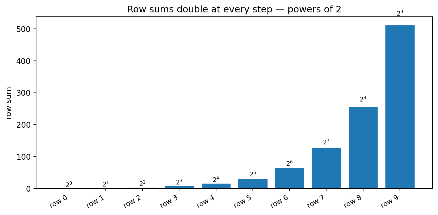
**Row sums.** Every row sum is a power of 2. This follows from the
**binomial theorem**: for any number $x$,
$$(1 + x)^n = \sum_{k=0}^{n} \binom{n}{k} x^k.$$
Setting $x = 1$ gives $2^n$ immediately. The bar chart below makes
the doubling pattern impossible to miss.
### Research Example: Does Every Row Sum to a Power of 2? {.unnumbered .unlisted}
Set $x = 1$ in the binomial theorem — the left side becomes $2^n$ immediately. Does the bar chart match that formula exactly for rows 0–9?
```{=latex}
\needspace{22\baselineskip}
```
```{python}
#| label: fig-pascal-rowsums
#| fig-cap: "Row sums of Pascal's triangle: every row doubles the previous, always reaching $2^n$."
import matplotlib.pyplot as plt

BLUE = '#1f77b4'

ns   = list(range(10))
sums = [2**n for n in ns]

fig, ax = plt.subplots(figsize=(8, 4))

bars = ax.bar(ns, sums, color=BLUE, edgecolor='white', linewidth=0.4)
for n_val, bar, s in zip(ns, bars, sums):
    ax.text(bar.get_x() + bar.get_width() / 2, s * 1.05,
            f'$2^{{{n_val}}}$', ha='center', va='bottom', fontsize=8)

ax.set_xticks(ns)
ax.set_xticklabels([f'row {n}' for n in ns], rotation=30, ha='right', fontsize=9)
ax.set_ylabel('row sum')
ax.set_title('Row sums double at every step — powers of 2', fontsize=12)
plt.tight_layout()
plt.show()
```
Every bar is exactly double the previous — the binomial theorem delivers a perfect power-of-2 proof with no computation required.
Let us verify the expansion symbolically with SymPy:
```{python}
from sympy import symbols, expand

x = symbols('x')
for n in range(6):
    print(f"(1+x)^{n} = {expand((1 + x)**n)}")
```
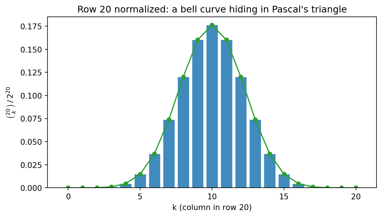
The coefficients in each expansion are exactly the entries of the
corresponding row of Pascal's triangle. Normalize row 20 by $2^{20}$
and plot it: a bell curve emerges, foreshadowing the Central Limit
Theorem that governs probability.
### Research Example: Does a Bell Curve Hide Inside Pascal's Triangle? {.unnumbered .unlisted}
Divide every entry in row 20 by $2^{20}$ to get a probability distribution — does the shape match the famous bell curve?
```{=latex}
\needspace{22\baselineskip}
```
```{python}
#| label: fig-pascal-bell
#| fig-cap: "Row 20 normalized by $2^{20}$: Pascal's triangle secretly contains the bell curve of probability."
import math
import matplotlib.pyplot as plt

BLUE  = '#1f77b4'
GREEN = '#2ca02c'

n_bell = 20
ks    = list(range(n_bell + 1))
probs = [math.comb(n_bell, k) / 2**n_bell for k in ks]

fig, ax = plt.subplots(figsize=(7, 4))

ax.bar(ks, probs, color=BLUE, edgecolor='white', linewidth=0.3, alpha=0.85)
ax.plot(ks, probs, 'o-', color=GREEN, markersize=5, lw=1.5)
ax.set_xlabel('k (column in row 20)')
ax.set_ylabel(r'$\binom{20}{k}\,/\,2^{20}$')
ax.set_title("Row 20 normalized: a bell curve hiding in Pascal's triangle",
             fontsize=12)
plt.tight_layout()
plt.show()
```
The bars form a perfect bell — the same shape that governs coin flips, test scores, and measurement errors, hiding all along in one row of Pascal's triangle.
**Alternating sums.** Setting $x = -1$ in the binomial theorem gives
$(1 + (-1))^n = 0^n$. For $n \ge 1$ this is 0, so the even-column
sum always equals the odd-column sum.
```{python}
import math
for n in range(1, 8):
    alt = sum(
        (-1)**k * math.comb(n, k) for k in range(n + 1)
    )
    print(f"row {n} alternating sum = {alt}")
```
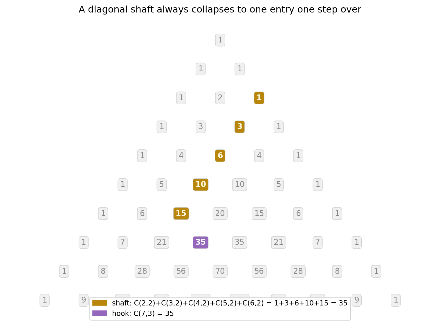
**Diagonals.** The rows hide secrets in their sums, but the diagonals
hold secrets of their own. Sum the entries along any diagonal starting
at a left-edge 1 — stepping one row down and one column to the right
at each step — and the total collapses to a single entry one step
further along. The figure below highlights one such collapse.
::: {.content-visible when-format="pdf"}
```{=latex}
\begin{center}
\begin{minipage}[c]{0.28\textwidth}\centering
\href{https://youtu.be/J0I1NuxUcpQ}{\includegraphics[width=\textwidth]{images/thumb_J0I1NuxUcpQ.jpg}}
\end{minipage}%
\hspace{0.02\textwidth}%
\begin{minipage}[c]{0.28\textwidth}
\small\textbf{Tipping Point Math}\\[3pt]
\small What You Don't Know About Pascal's Triangle\\[3pt]
\small\href{https://youtu.be/J0I1NuxUcpQ}{\texttt{youtu.be/J0I1NuxUcpQ}}
\end{minipage}%
\hspace{0.02\textwidth}%
\begin{minipage}[c]{0.36\textwidth}
\small Diagonal patterns, hockey-stick sums, and hidden sequences — a tour of Pascal's triangle secrets that most textbooks overlook.
\end{minipage}
\end{center}
```
:::
::: {.content-visible when-format="html"}
<div style="display:flex; align-items:flex-start; margin:1em 0; gap:12px; width:100%;">
<div style="flex:0 0 200px;"><a href="https://youtu.be/J0I1NuxUcpQ" target="_blank"><img src="https://img.youtube.com/vi/J0I1NuxUcpQ/0.jpg" style="width:100%;" alt="What You Don't Know About Pascal's Triangle"></a></div>
<div style="flex:1; font-size:0.85em;"><strong>Tipping Point Math</strong><br>What You Don't Know About Pascal's Triangle<br><a href="https://youtu.be/J0I1NuxUcpQ" target="_blank" style="font-family:monospace;">youtu.be/J0I1NuxUcpQ</a></div>
<div style="flex:1; font-size:0.85em;">Diagonal patterns, hockey-stick sums, and hidden sequences — a tour of Pascal's triangle secrets that most textbooks overlook.</div>
</div>
:::
Consider the diagonal with $r = 2$: the entries $\binom{2}{2}$,
$\binom{3}{2}$, $\binom{4}{2}$, $\binom{5}{2}$, $\binom{6}{2}$
(highlighted gold below) sum to $\binom{7}{3}$ — a single purple
entry one step over. Research topic 7 asks you to prove why this
pattern holds and to give it its famous name.
### Research Example: What Happens When You Add Up a Diagonal Shaft? {.unnumbered .unlisted}
Add five consecutive diagonal entries starting at $\binom{2}{2}$ — does the total collapse to a single entry one step over?
```{=latex}
\needspace{30\baselineskip}
```
```{python}
#| label: fig-pascal-diagonal
#| fig-cap: "A diagonal shaft of entries (gold) collapses to one hook entry (purple). Research topic 7 asks you to prove this identity and discover its name."
import matplotlib.pyplot as plt
import matplotlib.patches as mpatches

PURPLE = '#9467bd'

N_d = 10
tri_d = [[1]]
for i in range(1, N_d):
    prev = tri_d[-1]
    tri_d.append([1] + [prev[j] + prev[j+1] for j in range(i - 1)] + [1])

shaft = {(i, 2) for i in range(2, 7)}
hook  = (7, 3)

fig, ax = plt.subplots(figsize=(8, 6))

for n, row in enumerate(tri_d):
    for k, val in enumerate(row):
        x = k - n / 2.0
        y = float(N_d - 1 - n)
        if (n, k) in shaft:
            fc, tc, bold = '#b8860b', '#fff8dc', True
        elif (n, k) == hook:
            fc, tc, bold = PURPLE, 'white', True
        else:
            fc, tc, bold = '#f0f0f0', '#888888', False
        ax.text(x, y, str(val), ha='center', va='center',
                fontsize=10, color=tc,
                fontweight='bold' if bold else 'normal',
                bbox=dict(boxstyle='round,pad=0.3', facecolor=fc,
                          edgecolor='#cccccc', linewidth=0.5))

ax.set_xlim(-5.5, 5.5)
ax.set_ylim(-0.8, N_d - 0.2)
ax.axis('off')
gold   = mpatches.Patch(color='#b8860b',
    label='shaft: C(2,2)+C(3,2)+C(4,2)+C(5,2)+C(6,2) = 1+3+6+10+15 = 35')
purple = mpatches.Patch(color=PURPLE, label='hook: C(7,3) = 35')
ax.legend(handles=[gold, purple], loc='lower center', fontsize=9, framealpha=0.9)
ax.set_title('A diagonal shaft always collapses to one entry one step over',
             fontsize=12, pad=6)
plt.tight_layout()
plt.show()
```
Five separate entries along the shaft collapse to a single hook entry with the same value — the hockey stick identity in one picture.
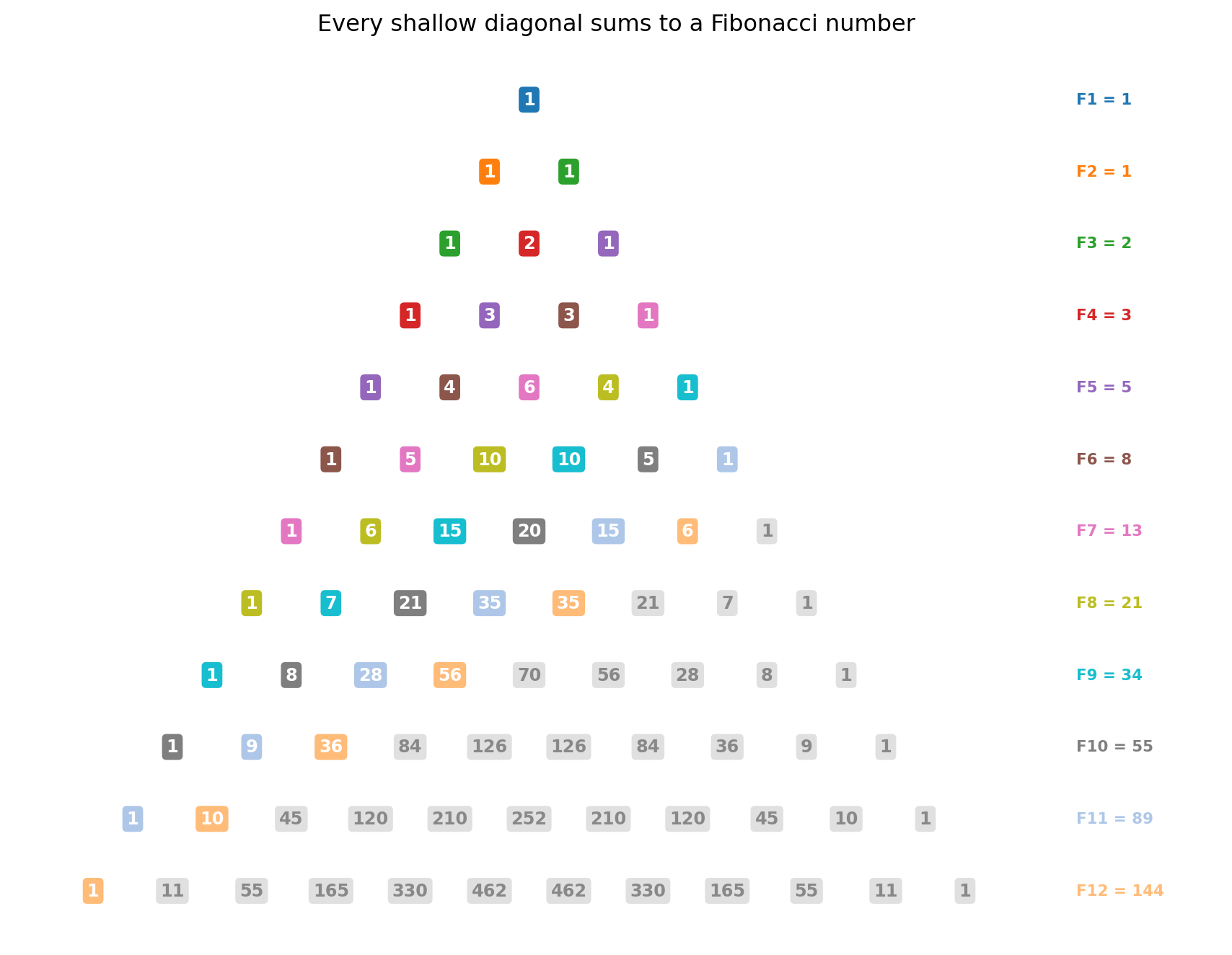
Now look along the *shallow* diagonals — the ones that cut across the
rows at a gentler angle. A completely different famous sequence hides
along these slanted paths, and the figure below makes it impossible to
miss. Research topic 3 asks you to prove why.
### Research Example: Do Fibonacci Numbers Hide Along Pascal's Diagonals? {.unnumbered .unlisted}
Color each shallow diagonal a different hue and sum its entries — does the sequence of sums ring a bell?
```{=latex}
\needspace{28\baselineskip}
```
```{python}
#| label: fig-pascal-fibonacci
#| fig-cap: "Shallow diagonals of Pascal's triangle (each colour is one diagonal) sum to successive Fibonacci numbers. The same triangle that hides powers of 2 in its rows hides the Fibonacci sequence in its diagonals."
import matplotlib.pyplot as plt

PALETTE = ['#1f77b4', '#ff7f0e', '#2ca02c', '#d62728', '#9467bd',
           '#8c564b', '#e377c2', '#bcbd22', '#17becf', '#7f7f7f',
           '#aec7e8', '#ffbb78']

def pascal(rows):
    tri = [[1]]
    for n in range(1, rows):
        p = tri[-1]
        tri.append([1] + [p[k] + p[k+1] for k in range(n-1)] + [1])
    return tri

def fib_seq(m):
    a, b, seq = 1, 1, []
    for _ in range(m):
        seq.append(a); a, b = b, a + b
    return seq

N    = 12
tri  = pascal(N)
fibs = fib_seq(N + 1)

fig, ax = plt.subplots(figsize=(9, 7))

for n, row in enumerate(tri):
    for k, val in enumerate(row):
        d  = n + k
        fc = PALETTE[d] if d < len(PALETTE) else '#e0e0e0'
        tc = 'white'    if d < len(PALETTE) else '#888888'
        x  = k - n / 2.0
        y  = float(N - 1 - n)
        ax.text(x, y, str(val), ha='center', va='center',
                fontsize=9, color=tc, fontweight='bold',
                bbox=dict(boxstyle='round,pad=0.25', facecolor=fc,
                          edgecolor='none'))

x_ann = N / 2.0 + 0.9
for d in range(len(PALETTE)):
    cells = [(n, k) for n, row in enumerate(tri)
             for k in range(len(row)) if n + k == d]
    if not cells:
        continue
    s     = sum(tri[n][k] for n, k in cells)
    n_bot = max(n for n, _ in cells)
    y_ann = float(N - 1 - n_bot)
    ax.text(x_ann, y_ann, f'F{d+1} = {s}',
            ha='left', va='center', fontsize=8,
            color=PALETTE[d], fontweight='bold')

ax.set_xlim(-6.5, x_ann + 1.8)
ax.set_ylim(-0.7, N - 0.2)
ax.axis('off')
ax.set_title('Every shallow diagonal sums to a Fibonacci number', fontsize=12)
plt.tight_layout()
plt.show()
```
Every colored diagonal collapses to a single Fibonacci number — the same sequence from Chapter 5 hiding in a completely different part of the same triangle.
::: {.content-visible when-format="pdf"}
```{=latex}
\begin{center}
\begin{minipage}[c]{0.28\textwidth}\centering
\href{https://youtu.be/24u3Em5Ro_k}{\includegraphics[width=\textwidth]{images/thumb_24u3Em5Ro_k.jpg}}
\end{minipage}%
\hspace{0.02\textwidth}%
\begin{minipage}[c]{0.28\textwidth}
\small\textbf{MathsSmart}\\[3pt]
\small Fibonacci Numbers in Pascal's Triangle\\[3pt]
\small\href{https://youtu.be/24u3Em5Ro_k}{\texttt{youtu.be/24u3Em5Ro\_k}}
\end{minipage}%
\hspace{0.02\textwidth}%
\begin{minipage}[c]{0.36\textwidth}
\small Traces the shallow diagonals of Pascal's triangle to reveal the Fibonacci sequence hiding inside — a visual proof of an unexpected connection.
\end{minipage}
\end{center}
```
:::
::: {.content-visible when-format="html"}
<div style="display:flex; align-items:flex-start; margin:1em 0; gap:12px; width:100%;">
<div style="flex:0 0 200px;"><a href="https://youtu.be/24u3Em5Ro_k" target="_blank"><img src="https://img.youtube.com/vi/24u3Em5Ro_k/0.jpg" style="width:100%;" alt="Fibonacci Numbers in Pascal's Triangle"></a></div>
<div style="flex:1; font-size:0.85em;"><strong>MathsSmart</strong><br>Fibonacci Numbers in Pascal's Triangle<br><a href="https://youtu.be/24u3Em5Ro_k" target="_blank" style="font-family:monospace;">youtu.be/24u3Em5Ro_k</a></div>
<div style="flex:1; font-size:0.85em;">Traces the shallow diagonals of Pascal's triangle to reveal the Fibonacci sequence hiding inside — a visual proof of an unexpected connection.</div>
</div>
:::
## Coloring by Divisibility: The Sierpiński Pattern {#sec-pascal-sierpinski}
```{python}
#| echo: false
from pathlib import Path; import urllib.request
_d = Path('images'); _d.mkdir(exist_ok=True)
_p = _d / 'Polish_students_in_Gottingen.jpg'
if not _p.exists():
try: urllib.request.urlretrieve(
'https://upload.wikimedia.org/wikipedia/commons/5/57/Polish_students_in_G%C3%B6ttingen_1907.jpg',
_p)
except Exception: pass
```
::: {.content-visible when-format="pdf"}
```{=latex}
\begin{center}
\begin{minipage}[c]{0.42\textwidth}
\includegraphics[width=\textwidth]{images/Polish_students_in_Gottingen.jpg}
\end{minipage}%
\hspace{0.03\textwidth}%
\begin{minipage}[c]{0.38\textwidth}
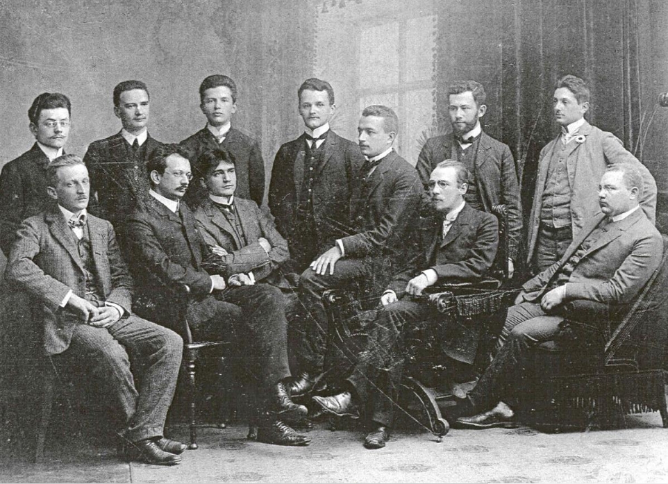
\small\textit{Wacław Sierpiński (1882--1969) appears among this group of Polish students in Göttingen, 1907.}\\[4pt]
\tiny Public domain, via Wikimedia Commons
\end{minipage}
\end{center}
```
:::
::: {.content-visible when-format="html"}
<div style="display:flex; align-items:center; margin:1em 0; gap:12px;">
<img src="images/Polish_students_in_Gottingen.jpg" style="width:200px; flex-shrink:0;" alt="Polish students in Göttingen 1907">
<div style="font-size:0.82em;"><em>Wacław Sierpiński (1882–1969) appears among this group of Polish students in Göttingen, 1907.</em><br><span style="font-size:0.85em;">Public domain, via Wikimedia Commons</span></div>
</div>
:::
Replace each entry with its remainder when divided by 2: entries
divisible by 2 become 0 (dark); odd entries become 1 (bright). The
`%` operator introduced in @sec-modular-operator performs this
reduction:
```{python}
# uses: tri
# Show Pascal mod 2 for the first 8 rows
for n, row in enumerate(tri):
    mod2_row = [c % 2 for c in row]
    print(f"row {n}: {mod2_row}")
```
A triangular pattern of 1s is emerging. For a larger triangle the
pattern becomes unmistakable. We build the grid mod 2 directly from
the recurrence — each entry is the sum of the two above it, taken
mod 2:
```{=latex}
\needspace{36\baselineskip}
```
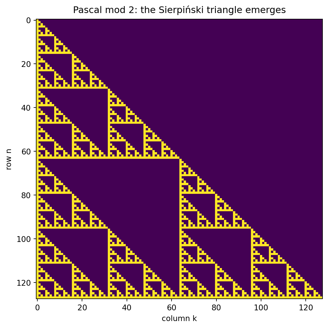
### Research Example: Does Pascal's Triangle Mod 2 Hide a Fractal? {.unnumbered .unlisted}
Color every odd entry bright and every even entry dark across 128 rows — does a recognizable fractal shape appear?
```{python}
#| label: fig-pascal-sierpinski
#| fig-cap: "Pascal's triangle mod 2, 128 rows. Every odd entry is bright; the Sierpiński triangle emerges — three self-similar copies nested inside each other, forever."
import numpy as np
import matplotlib.pyplot as plt

N = 128

mod2 = [[0] * N for _ in range(N)]
mod2[0][0] = 1
for n in range(1, N):
    for k in range(n + 1):
        a = mod2[n - 1][k - 1] if k > 0 else 0
        mod2[n][k] = (a + mod2[n - 1][k]) % 2

fig, ax = plt.subplots(figsize=(6, 6))
ax.imshow(np.array(mod2), cmap='viridis', interpolation='nearest', aspect='auto')
ax.set_title('Pascal mod 2: the Sierpiński triangle emerges', fontsize=12, pad=8)
ax.set_xlabel('column k')
ax.set_ylabel('row n')
plt.tight_layout()
plt.show()
```
Three copies of the same triangle nested inside a larger one — and each copy contains three more, and so on forever: a genuine fractal born from the simplest remainder rule [@borwein2006ema, §3.2].
The result is the **Sierpiński triangle** [@sierpinski1915]: a large triangle made of
three half-size copies of itself, each of which is made of three
quarter-size copies, and so on without end.
**Why does this happen?** A deep theorem called **Lucas's theorem** [@lucas1878]
explains it. For any prime $p$, write $n$ and $k$ in base $p$ with
digits $n_i$ and $k_i$. Then
$$\binom{n}{k} \equiv \prod_{i} \binom{n_i}{k_i} \pmod{p}.$$
For $p = 2$: $\binom{n}{k}$ is odd exactly when every binary digit of
$k$ is less than or equal to the corresponding binary digit of $n$.
In other words, $k$ must be a "binary sub-pattern" of $n$. The
fractal structure in the image is a direct consequence of this
digit-by-digit rule.
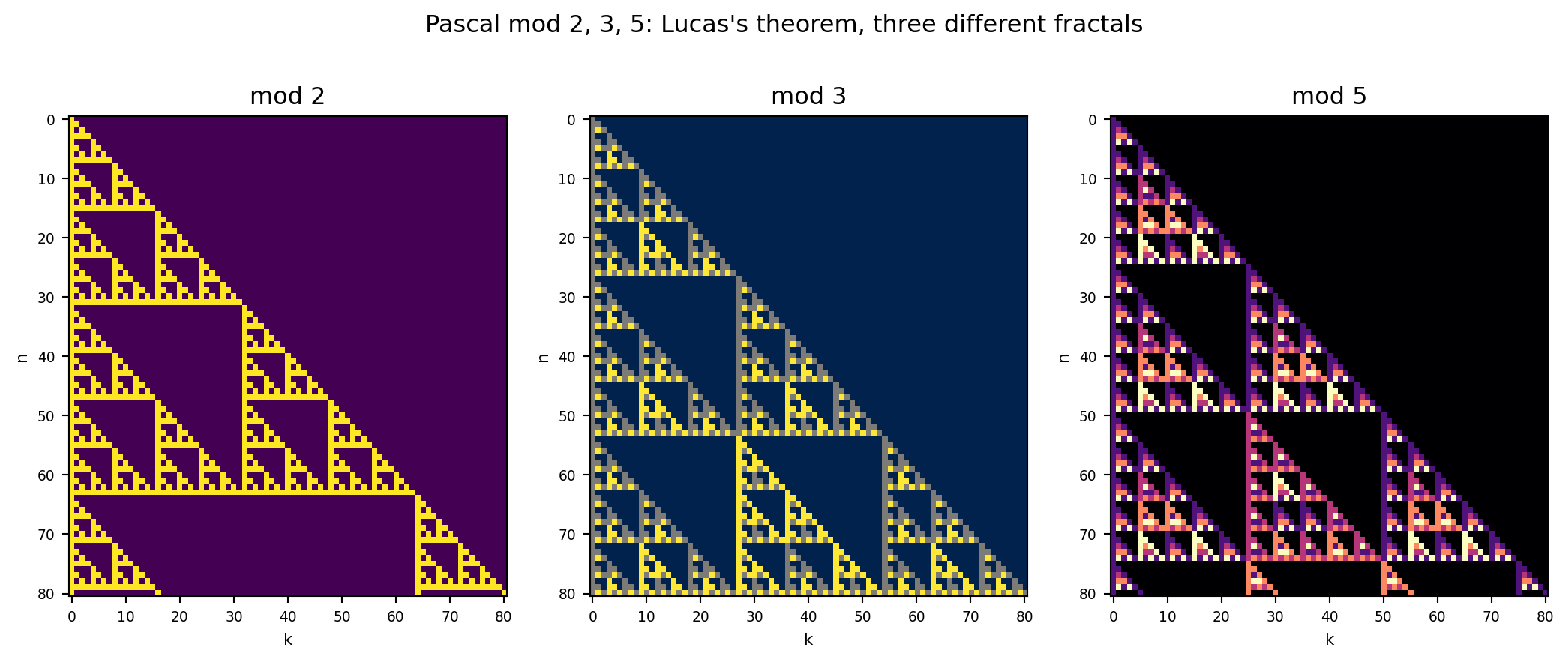
Lucas's theorem works for every prime, and every prime carves a
completely different fractal from the same grid. The figure below
places Pascal mod 2, mod 3, and mod 5 side by side.
### Research Example: Does Every Prime Carve Its Own Fractal? {.unnumbered .unlisted}
Place Pascal mod 2, mod 3, and mod 5 side by side across 81 rows — do the three primes produce visually distinct fractal patterns?
```{python}
#| label: fig-pascal-primes
#| fig-cap: "Lucas's theorem in action: Pascal mod $p$ for $p=2,3,5$. Each prime generates a distinct infinite fractal from the same triangle."
import math
import numpy as np
import matplotlib.pyplot as plt

M      = 81
primes = [2, 3, 5]
cmaps  = ['viridis', 'cividis', 'magma']

fig, axes = plt.subplots(1, 3, figsize=(11, 4.5))

for ax, p, cm in zip(axes, primes, cmaps):
    grid = np.zeros((M, M), dtype=int)
    for n in range(M):
        for k in range(n + 1):
            grid[n, k] = math.comb(n, k) % p
    ax.imshow(grid, cmap=cm, interpolation='nearest', aspect='auto')
    ax.set_title(f'mod {p}', fontsize=12)
    ax.set_xlabel('k', fontsize=8)
    ax.set_ylabel('n', fontsize=8)
    ax.tick_params(labelsize=7)

fig.suptitle("Pascal mod 2, 3, 5: Lucas's theorem, three different fractals",
             fontsize=12, y=1.01)
plt.tight_layout()
plt.show()
```
Every prime builds a completely different fractal from the same triangle — three primes, three distinct infinite patterns, all predicted by one theorem.
::: {.content-visible when-format="pdf"}
```{=latex}
\begin{center}
\begin{minipage}[c]{0.28\textwidth}\centering
\href{https://youtu.be/FnRhnZbDprE}{\includegraphics[width=\textwidth]{images/thumb_FnRhnZbDprE.jpg}}
\end{minipage}%
\hspace{0.02\textwidth}%
\begin{minipage}[c]{0.28\textwidth}
\small\textbf{Numberphile}\\[3pt]
\small A 1.58-Dimensional Object\\[3pt]
\small\href{https://youtu.be/FnRhnZbDprE}{\texttt{youtu.be/FnRhnZbDprE}}
\end{minipage}%
\hspace{0.02\textwidth}%
\begin{minipage}[c]{0.36\textwidth}
\small The Sierpi\'nski triangle emerges from Pascal's triangle mod 2 — and its fractal dimension is $\log_2 3 \approx 1.585$, not a whole number.
\end{minipage}
\end{center}
```
:::
::: {.content-visible when-format="html"}
<div style="display:flex; align-items:flex-start; margin:1em 0; gap:12px; width:100%;">
<div style="flex:0 0 200px;"><a href="https://youtu.be/FnRhnZbDprE" target="_blank"><img src="https://img.youtube.com/vi/FnRhnZbDprE/0.jpg" style="width:100%;" alt="A 1.58-Dimensional Object"></a></div>
<div style="flex:1; font-size:0.85em;"><strong>Numberphile</strong><br>A 1.58-Dimensional Object<br><a href="https://youtu.be/FnRhnZbDprE" target="_blank" style="font-family:monospace;">youtu.be/FnRhnZbDprE</a></div>
<div style="flex:1; font-size:0.85em;">The Sierpiński triangle emerges from Pascal's triangle mod 2 — and its fractal dimension is log₂ 3 ≈ 1.585, not a whole number.</div>
</div>
:::
The man behind this theorem was Édouard Lucas (1842–1891), a French
mathematician of dazzling range. He proved his theorem at 25, invented
the Tower of Hanoi puzzle, and designed a primality test for Mersenne
numbers that is still used today. His 1891 masterwork *Théorie des
nombres* gathered a lifetime of discoveries — and was published just
months before his death from a wound caused by a fragment of a broken
dinner plate at a banquet. He was 48.
## Estimating Fractal Dimension {#sec-pascal-dimension}
Ordinary shapes have integer dimensions: a line is 1-dimensional, a
square is 2-dimensional. But the Sierpiński triangle sits between
dimensions 1 and 2 — it has infinitely many points yet zero area.
Its **fractal dimension** captures exactly how much space it occupies.
**Self-similarity dimension.** The Sierpiński triangle is made of 3
copies of itself, each scaled down by a factor of $1/2$. Whenever a
shape consists of $N$ self-similar copies each scaled by $r$, its
dimension satisfies
$$N = (1/r)^d \implies d = \frac{\log N}{\log(1/r)}.$$
Here $N = 3$ and $r = 1/2$, so
$$d = \frac{\log 3}{\log 2} \approx 1.585.$$
The Sierpiński triangle is more than a curve but less than a solid.
**Verifying with Pascal's triangle.** The first $2^s$ rows of
Pascal mod 2 contain exactly $3^s$ odd entries. We can verify this
and watch the dimension estimate stabilize:
```{python}
# uses: mod2
import math

for s in range(1, 8):
    n_rows = 2**s
    count = sum(sum(mod2[n]) for n in range(n_rows))
    dim = math.log(count) / math.log(n_rows)
    print(
        f"2^{s}={n_rows:3d} rows: "
        f"{count:5d} odd,  dim={dim:.4f}"
    )

print(f"\nlog(3)/log(2) = {math.log(3)/math.log(2):.4f}")
```
The count is exactly $3^s$ at every scale, so the dimension estimate
is not just approaching $\log 3 / \log 2$ — it equals it exactly.
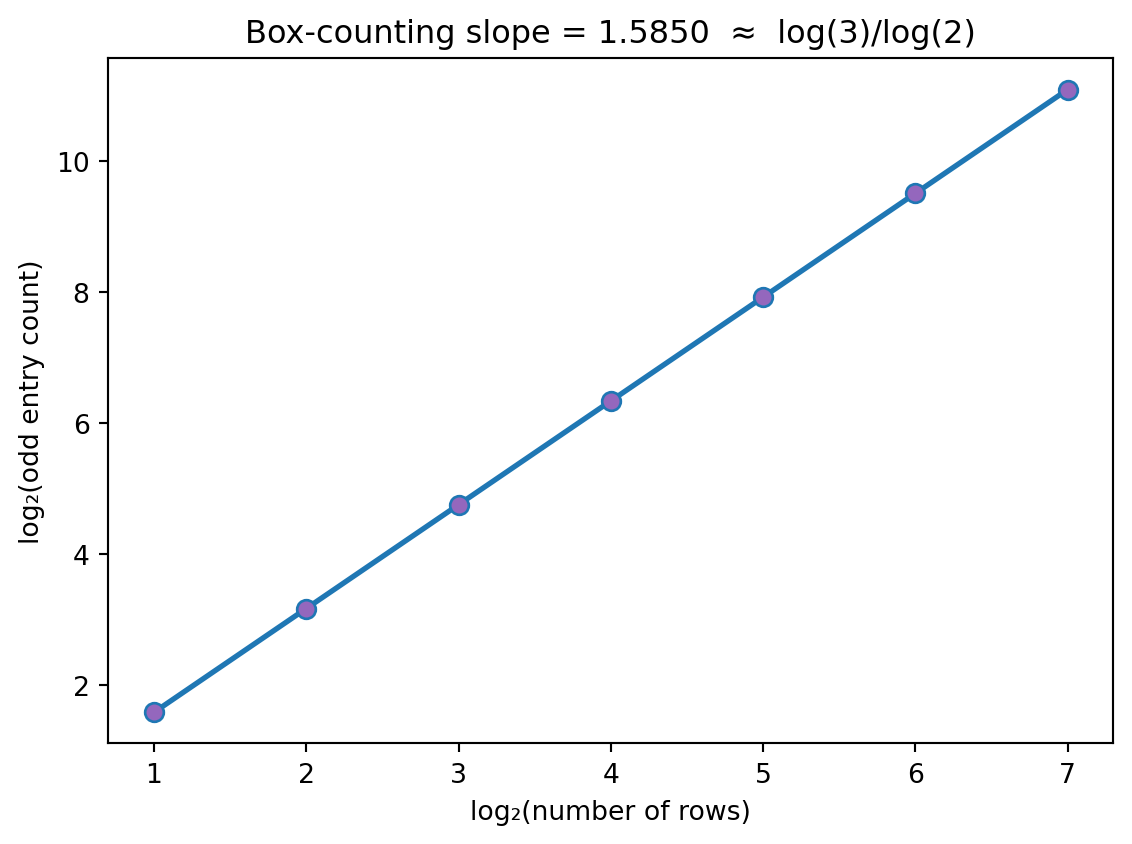
We can also visualize this as a **box-counting** log-log plot,
the standard method used for real-world fractal measurements:
### Research Example: Can We Measure the Sierpiński Triangle's Dimension? {.unnumbered .unlisted}
Plot log₂(odd-entry count) versus log₂(row count) for doublings $2^1$ through $2^7$ — does the slope land on $\log_2 3 \approx 1.585$?
```{=latex}
\needspace{22\baselineskip}
```
```{python}
#| label: fig-pascal-boxcount
#| fig-cap: "Box-counting log-log plot: the slope is the fractal dimension, confirming the Sierpiński triangle sits strictly between 1-dimensional and 2-dimensional."
import math
import matplotlib.pyplot as plt

BLUE   = '#1f77b4'
PURPLE = '#9467bd'

N = 128
mod2 = [[0] * N for _ in range(N)]
mod2[0][0] = 1
for n in range(1, N):
    for k in range(n + 1):
        a = mod2[n - 1][k - 1] if k > 0 else 0
        mod2[n][k] = (a + mod2[n - 1][k]) % 2

sizes  = [2**s for s in range(1, 8)]
counts = [sum(sum(mod2[n]) for n in range(sz)) for sz in sizes]

log_s = [math.log2(sz) for sz in sizes]
log_c = [math.log2(c)  for c  in counts]
slope = (log_c[-1] - log_c[0]) / (log_s[-1] - log_s[0])

fig, ax = plt.subplots(figsize=(6, 4.5))

ax.plot(log_s, log_c, 'o-', color=BLUE, lw=2, markersize=7,
        markerfacecolor=PURPLE)
ax.set_xlabel('log₂(number of rows)')
ax.set_ylabel('log₂(odd entry count)')
ax.set_title(f'Box-counting slope = {slope:.4f}  ≈  log(3)/log(2)', fontsize=12)
plt.tight_layout()
plt.show()
```
The slope hits $\log_2 3 \approx 1.585$ exactly — not approximately — proving the Sierpiński triangle lives precisely between a curve and a solid.
The slope of the log-log line is the fractal dimension. A slope of
1 would mean the odd entries form a 1-dimensional curve; a slope of 2
would mean they fill a 2-dimensional square. We get approximately
1.585, confirming the self-similarity calculation.
You will encounter this same number again in Chapter 12, where
box-counting is applied to more complex fractals like the Koch
snowflake and the Mandelbrot set.
## Further Research Topics {#sec-pascal-research}
1. **Prove the row-sum formula.** Every row of Pascal's triangle sums
to a power of 2. Confirm computationally for rows 0 through 20,
then prove it algebraically by substituting $x = 1$ into the
binomial theorem $(1 + x)^n = \sum_{k=0}^{n} \binom{n}{k} x^k$.
Next substitute $x = -1$ and prove that the alternating row sum
is 0 for all $n \ge 1$.
*(Problem proposed by Claude Code.)*
2. **Powers of 11.** Row $n$ encodes the digits of $11^n$: since
$11^n = (10+1)^n = \sum_{k=0}^{n} \binom{n}{k} 10^{n-k}$, the
binomial coefficients are the base-10 "digit groups" of $11^n$.
For $n \le 4$ no entry exceeds 9, so no carrying occurs and the
row entries are the exact decimal digits -- row 4 is
$[1, 4, 6, 4, 1]$ and $11^4 = 14641$. Verify computationally
that $\sum_{k=0}^n \binom{n}{k} \cdot 10^{n-k} = 11^n$ for
$n = 0$ through $30$. Why does $n = 5$ fail to give exact digits?
($\binom{5}{2} = 10$ forces a carry.) Explain why only finitely
many rows have this exact-digit property, using the fact that the
central entry $\binom{n}{\lfloor n/2 \rfloor}$ grows without
bound.
*(Problem proposed by Claude Code.)*
3. **Fibonacci numbers hiding in Pascal's triangle.** Sum Pascal's
entries along "shallow diagonals": the diagonal starting at
$\binom{n-1}{0}$, $\binom{n-2}{1}$, $\binom{n-3}{2}$, and so on,
summing as far as the index stays non-negative. Compute these sums
for $n = 1$ through $20$ and compare them to the Fibonacci numbers
from @sec-fib-rabbits. State a conjecture and verify it for
$n \le 50$.
*(Problem proposed by Claude Code.)*
4. **Rows with all odd entries.** Find every row index $n$ from 0 to
127 such that every entry in row $n$ is odd. List the values of
$n$ and express the pattern in terms of powers of 2. Then explain
your finding using Lucas's theorem: what property must the binary
representation of $n$ have?
*(Problem proposed by Claude Code.)*
5. **Counting odd entries per row.** For each $n$ from 0 to 100,
count how many entries in row $n$ are odd. Plot this count versus
$n$ and describe what you see. Write the count as a product
involving the binary digits of $n$. (Hint: if $n$ has binary
representation with digits $b_0, b_1, \ldots, b_r$, each equal
to 0 or 1, the count equals $\prod_i (b_i + 1)$.)
*(Problem proposed by Claude Code.)*
6. **GCD of a row's interior entries.** For $n \ge 2$, define
$g(n) = \gcd\!\bigl(\binom{n}{1}, \binom{n}{2}, \ldots,
\binom{n}{n-1}\bigr)$. Compute $g(n)$ for $n = 2$ through $60$
using Python's `math.gcd` together with `functools.reduce`. Make
a table of all $n$ with $g(n) > 1$, write each such $n$ in
factored form, and state a conjecture. You should find that
$g(n) = p$ exactly when $n$ is a power of the prime $p$, and
$g(n) = 1$ otherwise. Prove the simplest case: if $n = p$ is prime,
the formula $\binom{p}{k} = \frac{p(p-1)\cdots(p-k+1)}{k!}$ shows
that $p \mid \binom{p}{k}$ for $1 \le k \le p-1$ (the denominator
$k!$ has no factor of $p$ because $k < p$). Then investigate why
$g(p^2) = p$ rather than $p^2$: find the smallest $k$ for which
$p^2 \nmid \binom{p^2}{k}$ and explain the obstacle.
*(Problem proposed by Claude Code.)*
7. **Hockey stick identity.** The "hockey stick" identity states
$\sum_{i=r}^{n} \binom{i}{r} = \binom{n+1}{r+1}$. Verify it
computationally for $r = 3$ and $n = 5, 10, 15, 20$. Draw the
corresponding entries on a picture of Pascal's triangle to see why
the identity gets its name. Prove it by induction on $n$.
*(Problem proposed by Claude Code.)*
8. **Vandermonde's identity.** The identity
$\binom{m+n}{r} = \sum_{k=0}^{r} \binom{m}{k} \binom{n}{r-k}$
has a natural combinatorial proof: count the ways to choose $r$
people from a group of $m$ men and $n$ women. Verify the identity
computationally for all $m, n, r \le 12$ using `math.comb`.
*(Problem proposed by Claude Code.)*
9. **Alternating sums with higher powers.** Compute
$S_j(n) = \sum_{k=0}^{n} k^j \binom{n}{k}$ for $j = 0, 1, 2, 3$
and $n = 1$ through $10$. For each $j$, conjecture a closed form
for $S_j(n)$ in terms of $n$ and powers of 2. Prove at least the
case $j = 1$ using the identity
$k \binom{n}{k} = n \binom{n-1}{k-1}$.
*(Problem proposed by Claude Code.)*
10. **Singmaster's conjecture: how many times can a number appear?**
Most integers appear in Pascal's triangle only once (if they are
prime) or twice (on the symmetric edges), but some recur
surprisingly often. In 1971 David Singmaster conjectured [@singmaster1971] that
every integer greater than 1 appears at most a fixed, finite
number of times -- but no such bound has ever been proved.
Verify that 3003 holds the current record of 8 appearances:
show that $\binom{3003}{1} = \binom{78}{2} = \binom{15}{5} =
\binom{14}{6} = 3003$ (plus their mirror-image counterparts from
the triangle's symmetry). Write code that scans Pascal's triangle
through row 500, counts how many times each value appears, and
prints every value with 6 or more appearances. Extend the search
to row 2000 and report whether any value beats 3003's record of
8. The conjecture remains open: it is unknown whether any fixed
$N$ exists such that every integer appears at most $N$ times.
*(Problem proposed by Claude Code.)*
11. **Pascal mod 3.** Build a grid showing $C(n, k) \bmod 3$ for
$n = 0, 1, \ldots, 80$, coloring cells by three values (e.g.,
white, light gray, dark gray for 0, 1, 2). Describe the pattern.
Count non-zero entries in the first $3^s$ rows for $s = 1, \ldots,
5$ and estimate the fractal dimension. Is the answer
$\log N / \log 3$ for some integer $N$? What is $N$?
*(Problem proposed by Claude Code.)*
12. **Central binomial coefficients.** The middle entry of row $2n$
is $\binom{2n}{n}$: the values $1, 2, 6, 20, 70, 252, \ldots$
Stirling's approximation predicts $\binom{2n}{n} \approx 4^n /
\sqrt{\pi n}$. Verify this by computing and plotting the ratio
$\binom{2n}{n} \sqrt{\pi n} / 4^n$ for $n = 1$ through $50$.
Does it converge to 1? How quickly?
*(Problem proposed by Claude Code.)*
13. **Catalan numbers.** Define $C_n = \binom{2n}{n} / (n+1)$.
The sequence begins $1, 1, 2, 5, 14, 42, 132, \ldots$ Compute
the first 15 values and look up the sequence in the OEIS (the
Online Encyclopedia of Integer Sequences, which you will explore
in Chapter 8). Catalan numbers count the number of valid
expressions with $n$ pairs of parentheses -- for example, for
$n = 3$ the five valid strings are ()()(), ((())), (())(), ()(()),
and (()()). Write code that generates and counts all valid
parenthesis strings for small $n$ and verify the Catalan formula.
*(Problem proposed by Claude Code.)*
14. **Ballot problem and the reflection principle.**
$\binom{a+b}{a}$ counts all lattice paths from $(0,0)$ to
$(a, b)$ using unit steps right (R) and up (U). Interpret a
sequence of $a$ A-votes and $b$ B-votes (with $a > b \ge 1$) as
such a path: R for an A-vote, U for a B-vote. The ballot theorem [@bertrand1887]
states that the number of orderings in which A's running total
is strictly greater than B's at every step equals
$\dfrac{a-b}{a+b}\binom{a+b}{a}$. Write code that enumerates
all vote sequences for small $a, b$ and counts the "good" ones;
verify the formula for all pairs with $a + b \le 12$ and
$a > b \ge 1$. Then prove algebraically that
$\binom{a+b}{a} - \binom{a+b}{a-1} = \dfrac{a-b}{a+b}\binom{a+b}{a}$,
and argue (using the reflection principle: reflect each bad path
at its first touch of the diagonal $y = x$) that
$\binom{a+b}{a-1}$ counts the bad paths. How does the special
case $a = n+1$, $b = n$ connect to the Catalan numbers from
topic 13?
*(Problem proposed by Claude Code.)*
15. **Kummer's theorem** [@kummer1852]. The highest power of a prime $p$ that
divides $\binom{m+n}{m}$ equals the number of carries when you
add $m$ and $n$ in base $p$. Verify this for $p = 2$ and all
pairs $m, n \le 30$: compute the 2-adic valuation of
$\binom{m+n}{m}$ (how many times 2 divides it) and separately
count the number of carries when adding $m$ and $n$ in binary.
The two numbers should always agree.
*(Problem proposed by Claude Code.)*
16. **Fractal dimension for different primes.** For each prime
$p \in \{2, 3, 5, 7\}$, count the non-zero entries in the first
$p^s$ rows of Pascal mod $p$ for $s = 1, 2, 3, 4, 5$. Estimate
the fractal dimension in each case. Conjecture a formula: the
Sierpinski triangle for prime $p$ has dimension $\log(p(p+1)/2) /
\log(p)$. Check whether this formula is correct and, if so,
explain why $(p(p+1)/2)$ counts the non-zero entries in the first
$p$ rows.
*(Problem proposed by Claude Code.)*
17. **Lucas's theorem as fast code.** Write a function
`c_mod_p(n, k, p)` that computes $\binom{n}{k} \bmod p$ using
Lucas's theorem -- extract the base-$p$ digits of $n$ and $k$,
apply the product formula, and combine. Verify that it matches
`math.comb(n, k) % p` for all $n, k \le 200$ and $p \in \{2, 3,
5, 7\}$. Time both approaches for large $n$ and report the speedup.
*(Problem proposed by Claude Code.)*
18. **Pascal's tetrahedron.** Pascal's triangle generalizes to three
dimensions via the **trinomial coefficient**
$T(n;\,j,k) = \dfrac{n!}{j!\,k!\,(n-j-k)!}$
(for $j, k \ge 0$, $j+k \le n$), which is the coefficient of
$x^j y^k z^{n-j-k}$ in $(x+y+z)^n$. Verify this with SymPy's
`expand` for $n = 3$ and $n = 4$. Write code that displays layer
$n$ as a triangular array and confirm that the sum of all entries
in layer $n$ equals $3^n$. Build a 3D array of
$T(n;\,j,k) \bmod 2$ for $n \le 26$, visualize horizontal
slices, and describe the self-similar structure. Estimate the
fractal dimension of the set of positions where
$T(n;\,j,k) \not\equiv 0 \pmod{2}$ and compare it to the 2D
Sierpinski dimension of $\log_2 3 \approx 1.585$. As a further
challenge, state and verify a 3D analogue of Lucas's theorem
that predicts exactly when $T(n;\,j,k)$ is odd.
*(Problem proposed by Claude Code.)*
19. **Cellular automata connection.** "Rule 90" is a cellular
automaton where each cell's next state equals the XOR of its two
neighbors. Starting from a single occupied cell, run Rule 90 for
128 generations (one row per generation) and compare the output
side by side with the Pascal mod 2 grid built in this chapter.
Are they identical? Prove or disprove: the state of cell $k$ at
generation $n$ in Rule 90 equals $\binom{n}{k} \bmod 2$. (You
will explore cellular automata in depth in Chapter 10.)
*(Problem proposed by Claude Code.)*
20. **Wolstenholme's theorem** [@wolstenholme1862]. For any prime $p \ge 5$, the central
binomial coefficient satisfies $\binom{2p}{p} \equiv 2 \pmod{p^3}$.
Verify this for all primes $5 \le p \le 23$ by computing
$\binom{2p}{p} \bmod p^3$ with `math.comb`. A
**Wolstenholme prime** is a prime where the even stronger
congruence $\binom{2p}{p} \equiv 2 \pmod{p^4}$ holds. The only
known Wolstenholme primes below $10^9$ are 16843 and 2124679.
Verify that both satisfy the stronger congruence. Extend the
search as far as your computer allows -- no third Wolstenholme
prime has ever been found, and it is an open question whether any
more exist.
*(Problem proposed by Claude Code.)*