# Fractals: Infinite Detail at Every Scale {#sec-fractals}
## Shapes That Repeat at Every Scale {#sec-fractals-intro}
```{python}
#| echo: false
from pathlib import Path; import urllib.request
_d = Path('images'); _d.mkdir(exist_ok=True)
for _fn, _url in [
('mandelbrot.jpg', 'https://upload.wikimedia.org/wikipedia/commons/1/19/Benoit_Mandelbrot_mg_1804.jpg'),
('cantor.jpg', 'https://upload.wikimedia.org/wikipedia/commons/e/e7/Georg_Cantor2.jpg'),
]:
_p = _d / _fn
if not _p.exists():
try: urllib.request.urlretrieve(_url, _p)
except Exception: pass
```
::: {.content-visible when-format="pdf"}
```{=latex}
\begin{center}
\begin{minipage}[t]{0.40\textwidth}\centering
\includegraphics[width=0.70\textwidth]{images/mandelbrot.jpg}\\[4pt]
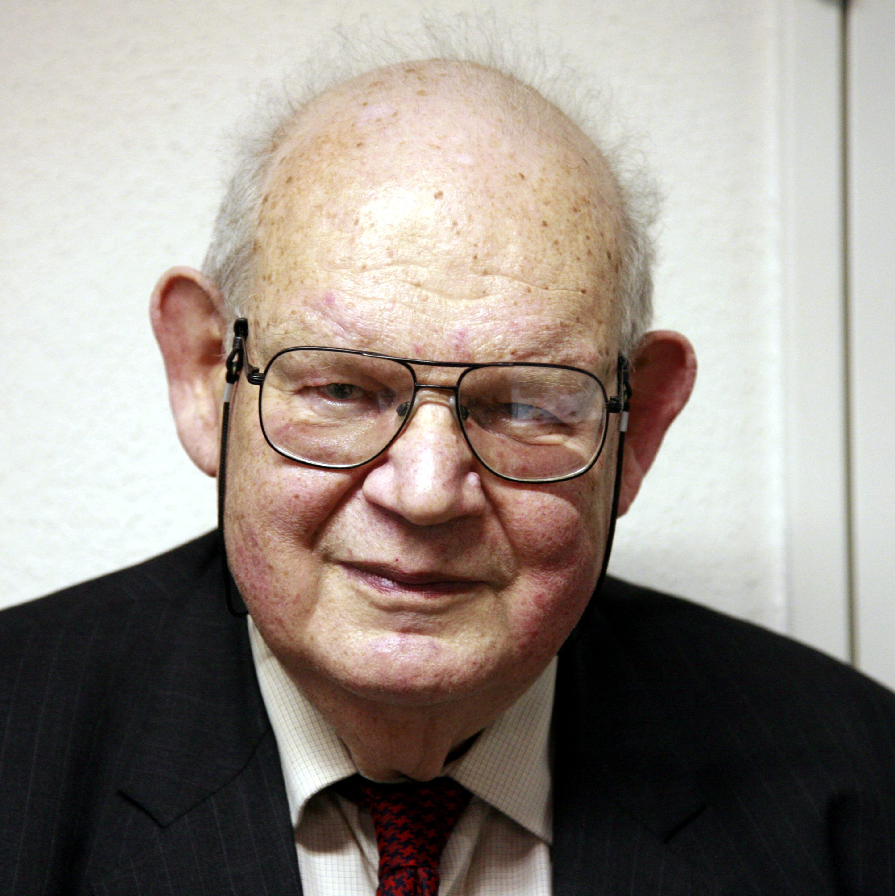
\small\textit{Benoît Mandelbrot (1924--2010)}\\[2pt]
\tiny CC BY-SA 2.0 fr, Rama, via Wikimedia Commons
\end{minipage}%
\hspace{0.04\textwidth}%
\begin{minipage}[t]{0.40\textwidth}\centering
\includegraphics[width=0.70\textwidth]{images/cantor.jpg}\\[4pt]
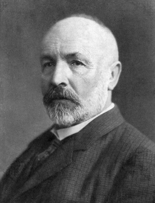
\small\textit{Georg Cantor (1845--1918)}\\[2pt]
\tiny Public domain, via Wikimedia Commons
\end{minipage}
\end{center}
```
:::
::: {.content-visible when-format="html"}
<div style="display:flex; justify-content:center; gap:24px; margin:1em 0; flex-wrap:wrap;">
<div style="text-align:center; max-width:160px;">
<img src="images/mandelbrot.jpg" style="width:120px;" alt="Benoît Mandelbrot"><br>
<em style="font-size:0.82em;">Benoît Mandelbrot (1924–2010)</em><br>
<span style="font-size:0.72em;">CC BY-SA 2.0 fr, Rama, via Wikimedia Commons</span>
</div>
<div style="text-align:center; max-width:160px;">
<img src="images/cantor.jpg" style="width:120px;" alt="Georg Cantor"><br>
<em style="font-size:0.82em;">Georg Cantor (1845–1918)</em><br>
<span style="font-size:0.72em;">Public domain, via Wikimedia Commons</span>
</div>
</div>
:::
Zoom in on a photograph of a mountain range and you might mistake
a small rocky hillside for the full panorama.
Zoom in on a coastline and a ten-meter stretch of shore
looks like the whole continent's edge.
Zoom in on a fern leaf and you find smaller leaves
shaped just like the whole.
These are not accidents; they are **self-similar structures**,
shapes in which every part resembles the whole at a smaller scale.
Classical geometry gives us circles and squares whose smooth curves
and straight edges become featureless when you look closely enough.
Self-similar shapes are different: they have detail at every scale,
never becoming smooth or flat.
The mathematician Benoit Mandelbrot coined the word **fractal** in 1975
for this family of shapes, and a generation of computer experiments
turned them from curiosities into a major branch of mathematics [@mandelbrot1975].
The simplest fractal is the **Cantor set**, invented by Georg Cantor
in 1883 [@cantor1883].
Start with the interval $[0, 1]$.
Remove the open middle third $(1/3, 2/3)$, leaving two intervals.
Remove the middle third of each of those, leaving four intervals.
Continue forever.
The Cantor set is whatever survives.
At depth $d$ there are $2^d$ intervals, each of length $(1/3)^d$.
The total length is $(2/3)^d$, which shrinks to zero.
Yet infinitely many points survive -- every endpoint of every
interval, for instance.
The Cantor set is simultaneously "too big to ignore" and
"so thin it has length zero," a paradox that troubled 19th-century
mathematicians but is perfectly natural for a fractal.
### Research Example: How Does the Cantor Set Disappear? {.unnumbered .unlisted}
Each step erases the middle third of every surviving piece. Can we see the thinning happen step by step — and does the picture capture what it means for something to have "length zero but infinitely many points"?
```{python}
intervals = [(0.0, 1.0)]
for depth in range(6):
    n = len(intervals)
    total = sum(b - a for a, b in intervals)
    print(f"Depth {depth}: {n:>2} intervals, "
          f"total length {total:.4f}")
    new_ivs = []
    for a, b in intervals:
        t = (b - a) / 3
        new_ivs.extend([(a, a + t), (b - t, b)])
    intervals = new_ivs
```
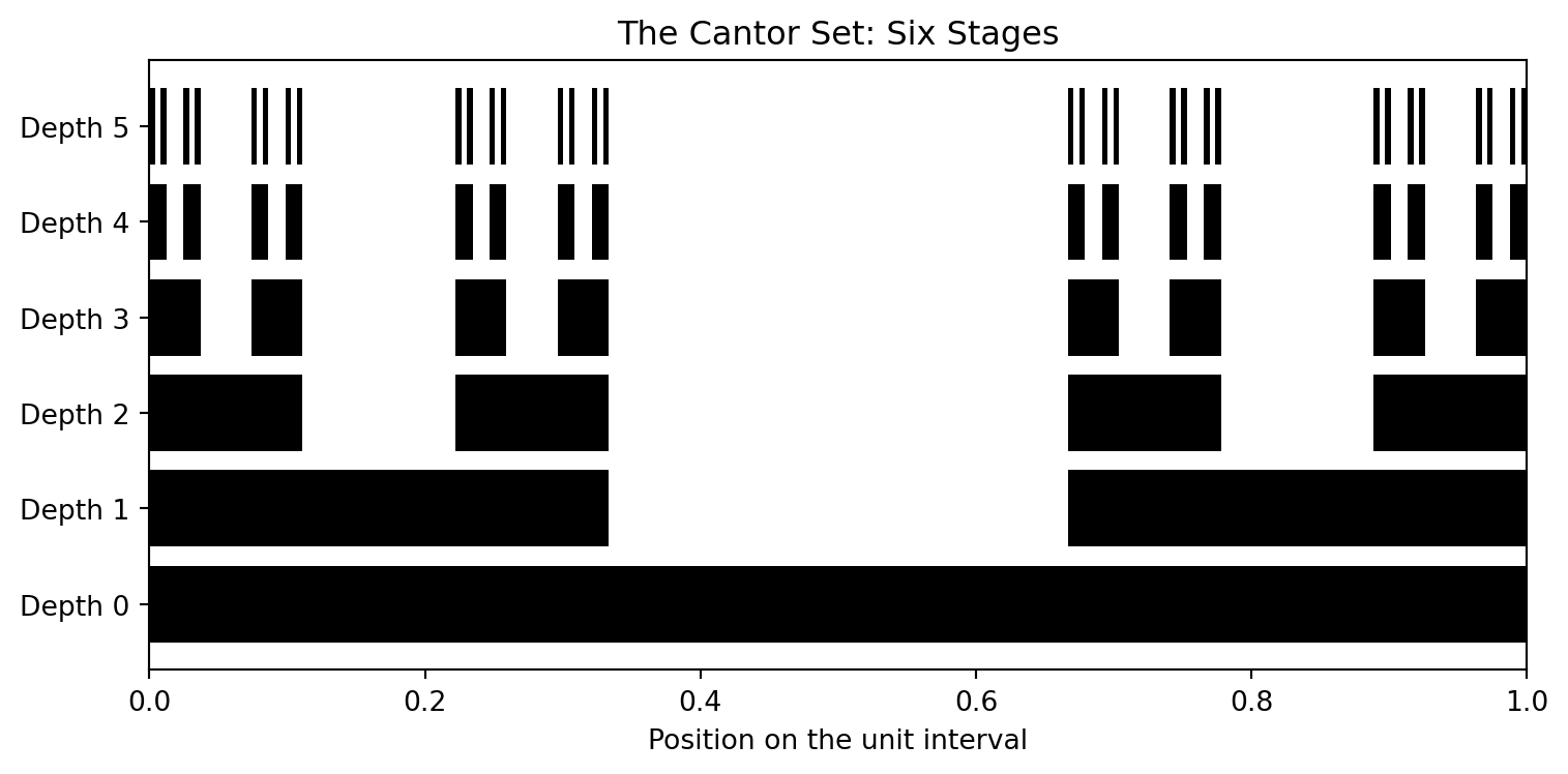
Each row of the strip chart below shows one depth.
Each black bar is a surviving interval.
As the depth grows the bars thin and multiply,
converging toward something that is neither a solid interval
nor an empty set.
```{python}
import matplotlib.pyplot as plt

stages = []
ivs = [(0.0, 1.0)]
stages.append(ivs[:])
for _ in range(5):
    nxt = []
    for a, b in ivs:
        t = (b - a) / 3
        nxt.extend([(a, a + t), (b - t, b)])
    ivs = nxt
    stages.append(ivs[:])

fig, ax = plt.subplots(figsize=(8, 4))
for depth, ivs_d in enumerate(stages):
    for a, b in ivs_d:
        ax.broken_barh(
            [(a, b - a)],
            (depth - 0.4, 0.8),
            facecolors='black'
        )
ax.set_yticks(range(6))
ax.set_yticklabels(
    [f'Depth {d}' for d in range(6)]
)
ax.set_xlim(0, 1)
ax.set_xlabel('Position on the unit interval')
ax.set_title('The Cantor Set: Six Stages')
plt.tight_layout()
plt.show()
```
The bars multiply and thin with every step, yet each depth inherits the exact structure of the one above it. This is the Cantor set materializing — something that shrinks to zero total length while preserving infinitely many points and an endlessly repeating pattern.
## Iterated Function Systems {#sec-fractals-ifs}
A fractal can be built from a small set of rules,
each one a "shrink-and-shift" operation applied to the
current picture.
Mathematicians call such a ruleset an
**iterated function system (IFS)** [@barnsley1988].
The key theorem is that any IFS with contracting maps has a
unique **attractor** -- a shape that is mapped to itself
by the whole collection of rules.
Here is an IFS for the Sierpinski triangle
with three rules, one per vertex of an equilateral triangle.
| Rule | Operation |
|------|-----------|
| $w_1$ | Move halfway from current point to vertex 1 |
| $w_2$ | Move halfway from current point to vertex 2 |
| $w_3$ | Move halfway from current point to vertex 3 |
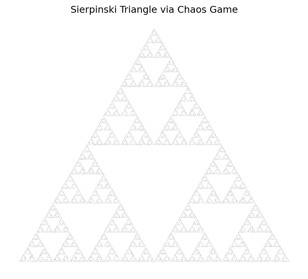
Apply one rule chosen **at random** at each step,
plot the resulting point, and repeat 50,000 times.
This is the **chaos game**: a random algorithm whose long-run
output is completely deterministic -- it always draws the
same Sierpinski triangle [@sierpinski1915].
We saw the Sierpinski pattern emerge from Pascal's triangle
in @sec-pascal-sierpinski.
Here it appears from a completely different direction --
from random chance applied to three simple rules.
The new Python tool here is `random.choice(seq)`,
which picks one element from the sequence `seq` uniformly
at random.
`random.seed` and `random.randint` were introduced at
@sec-automata-symmetry; `random.choice` follows the same
pattern but picks from any sequence, not just integers.
### Research Example: What Shape Does Randomness Draw? {.unnumbered .unlisted}
Pick any vertex of a triangle at random, move halfway there, and plot the point. Repeat 50,000 times with no drawing instructions whatsoever. Does the cloud of random dots converge to a recognizable shape — and is it always the same one, no matter where you start?
```{python}
import random
import matplotlib.pyplot as plt

random.seed(42)
verts = [(0.0, 0.0), (1.0, 0.0), (0.5, 3**0.5 / 2)]
x, y = verts[0]
xs, ys = [], []
for _ in range(50_000):
    vx, vy = random.choice(verts)
    x = (x + vx) / 2
    y = (y + vy) / 2
    xs.append(x)
    ys.append(y)

fig, ax = plt.subplots(figsize=(6, 5))
ax.plot(xs, ys, ',k', alpha=0.15, markersize=1)
ax.set_aspect('equal')
ax.set_title('Sierpinski Triangle via Chaos Game')
ax.axis('off')
plt.tight_layout()
plt.show()
```
Run this and 50,000 randomly placed dots assemble into
an unmistakable triangle of triangles of triangles.
The attractor is the same object discovered by Sierpinski in 1915,
and the same pattern that appeared in Pascal's triangle mod 2 --
three completely different paths to the same shape.
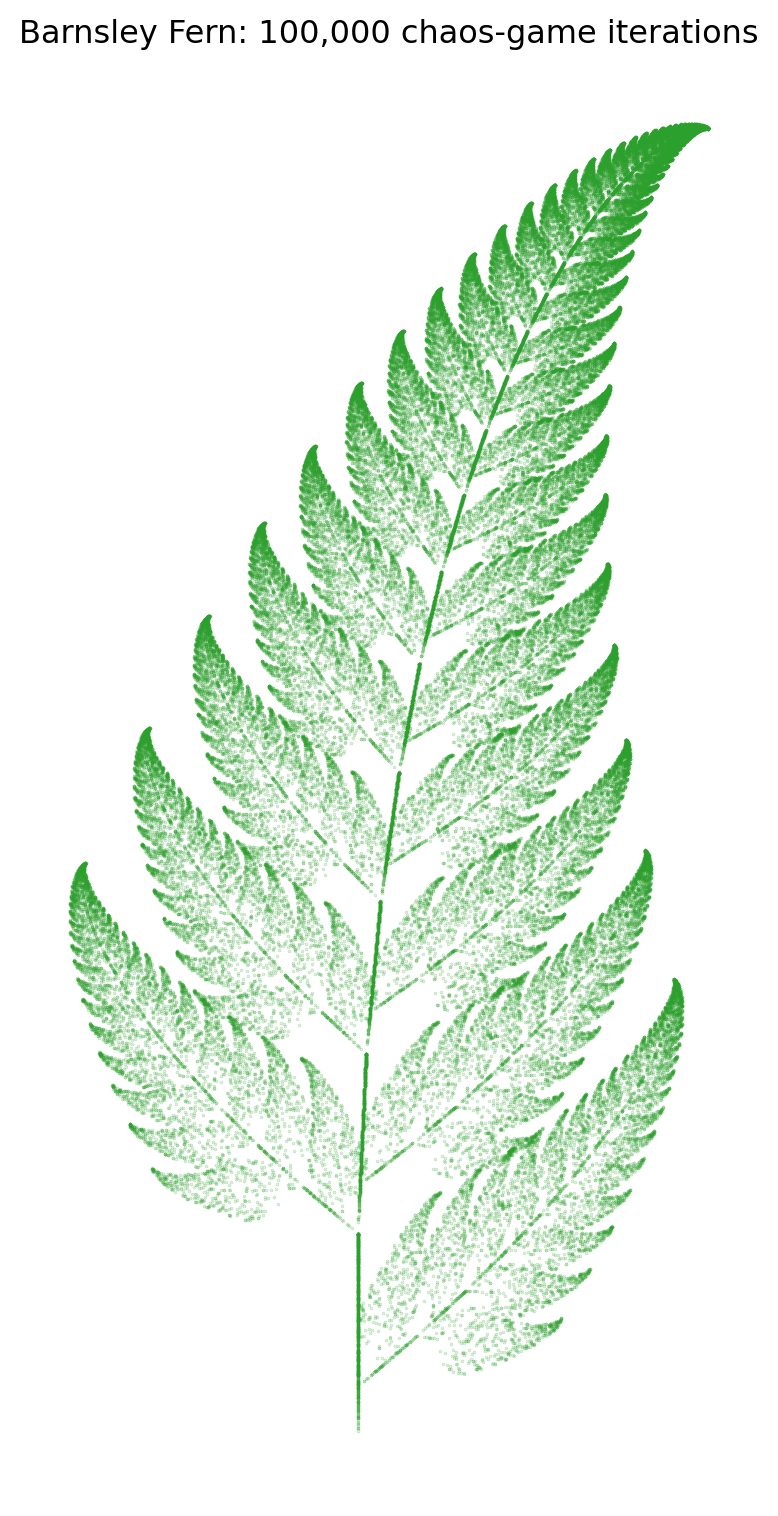
### Research Example: Can Four Rules Build a Plant? {.unnumbered .unlisted}
The Sierpinski triangle is not the only shape hiding inside such a rule.
Four affine transformations — a stem, two side leaflets, and a main blade —
assemble something unmistakably botanical.
Can four simple "shrink-and-shift" rules, applied at random, produce something you would recognize as a fern?
```{python}
#| label: fig-fractals-fern
#| fig-cap: "Barnsley fern: 100,000 chaos-game iterations of four affine transformations. No drawing commands — pure probability assembling a plant."
import matplotlib.pyplot as plt
import random
GREEN = '#2ca02c'

random.seed(42)
transforms = [
    ((0, 0, 0, 0.16), (0, 0), 0.01),
    ((0.85, 0.04, -0.04, 0.85), (0, 1.6), 0.85),
    ((0.2, -0.26, 0.23, 0.22), (0, 1.6), 0.07),
    ((-0.15, 0.28, 0.26, 0.24), (0, 0.44), 0.07),
]
x, y = 0.0, 0.0
xs_fern, ys_fern = [], []
for _ in range(100_000):
    r = random.random()
    cumul = 0.0
    for (a, b, c, d), (tx, ty), p in transforms:
        cumul += p
        if r < cumul:
            x, y = a*x + b*y + tx, c*x + d*y + ty
            break
    xs_fern.append(x)
    ys_fern.append(y)
fig, ax = plt.subplots(figsize=(5, 8))
ax.scatter(xs_fern, ys_fern, s=0.1, color=GREEN, alpha=0.3)
ax.set_aspect('equal')
ax.set_title("Barnsley Fern: 100,000 chaos-game iterations")
ax.axis('off')
fig.tight_layout()
plt.show()
```
No drawing commands, no bezier curves, no coordinates — just four probabilities and a loop. The fern's leaflets, stem, and overall silhouette emerge purely from the mathematics of contraction, a reminder that nature's most intricate patterns can hide inside very simple rules.
## The Koch Snowflake {#sec-fractals-koch}
```{python}
#| echo: false
from pathlib import Path; import urllib.request
_d = Path('images'); _d.mkdir(exist_ok=True)
_p = _d / 'koch.jpg'
if not _p.exists():
try: urllib.request.urlretrieve('https://upload.wikimedia.org/wikipedia/commons/0/0e/Helge_von_Koch.jpg', _p)
except Exception: pass
```
::: {.content-visible when-format="pdf"}
```{=latex}
\begin{center}
\begin{minipage}[c]{0.22\textwidth}
\includegraphics[width=\textwidth]{images/koch.jpg}
\end{minipage}%
\hspace{0.03\textwidth}%
\begin{minipage}[c]{0.55\textwidth}
\small\textit{Helge von Koch (1870--1924)}\\[2pt]
\tiny Public domain, via Wikimedia Commons
\end{minipage}
\end{center}
```
:::
::: {.content-visible when-format="html"}
<div style="display:flex; align-items:center; margin:1em 0; gap:12px;">
<img src="images/koch.jpg" style="width:100px; flex-shrink:0;" alt="Helge von Koch">
<div style="font-size:0.82em;"><em>Helge von Koch (1870–1924)</em><br><span style="font-size:0.85em;">Public domain, via Wikimedia Commons</span></div>
</div>
:::
In 1904 the Swedish mathematician Helge von Koch constructed
a curve designed to be **continuous but nowhere differentiable**:
it has no tangent line at any point [@koch1904].
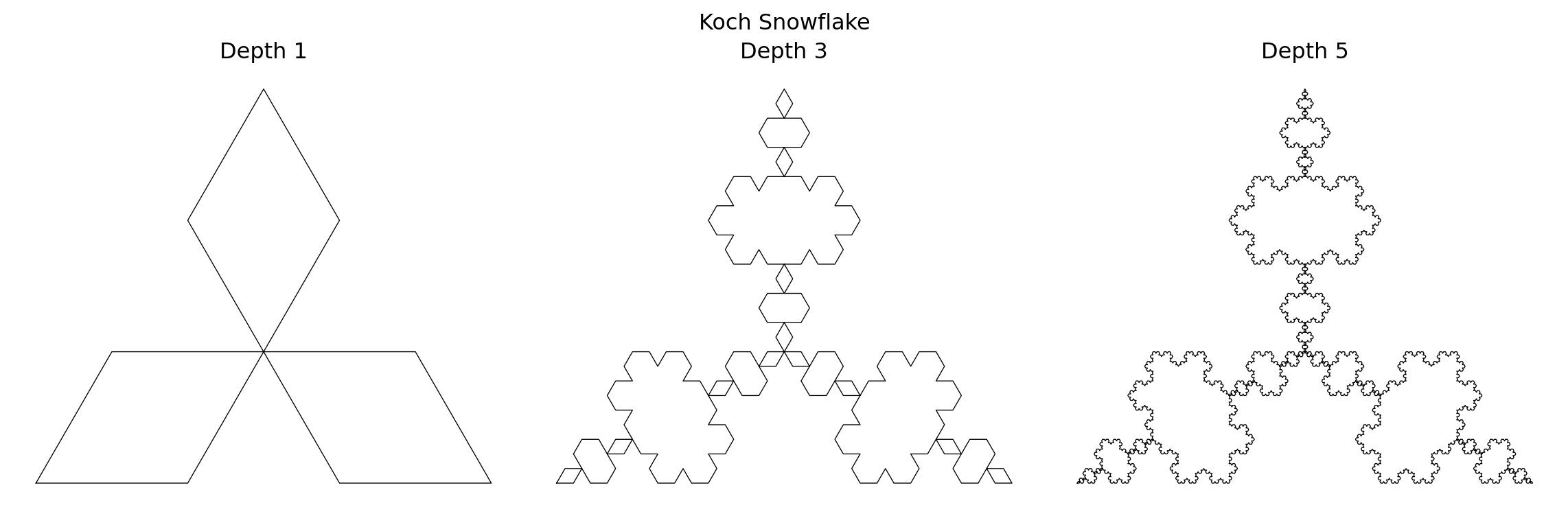
The construction is purely geometric.
**Step 0.** Start with an equilateral triangle.
**Step 1.** Divide each edge into three equal thirds.
Remove the middle third and replace it with two sides of an
equilateral triangle pointing outward.
Each edge is now four segments, each one-third the original length.
**Step 2.** Apply Step 1 to every segment.
**Continue forever.**
After $d$ steps the snowflake boundary has
$3 \times 4^d$ segments, each of length $(1/3)^d$.
The perimeter is therefore
$$P_d = 3 \times 4^d \times \left(\frac{1}{3}\right)^d
= 3 \times \left(\frac{4}{3}\right)^d.$$
Since $4/3 > 1$ the perimeter **grows without bound**,
even though the snowflake fits inside a bounded region.
Infinite perimeter, finite area -- a paradox that is perfectly
natural for a fractal.
### Research Example: Does the Perimeter Really Grow Without Bound? {.unnumbered .unlisted}
Each step multiplies the number of segments by 4 and shrinks their length by 3, so the perimeter grows by a factor of 4/3 each time. Can we watch the perimeter blow up numerically — and draw the snowflake at three levels of detail to see what "infinite perimeter, finite area" looks like?
To draw the snowflake we represent each point as a Python complex
number. The peak of the outward equilateral triangle is obtained
by rotating the middle-third segment vector by $60°$ counterclockwise.
Rotating a complex number by $60°$ multiplies it by
$\cos 60° + i \sin 60° = 0.5 + i\frac{\sqrt{3}}{2}$.
```{python}
import math

def koch_step(pts):
    out = []
    cos60, sin60 = 0.5, 3**0.5 / 2
    for i in range(len(pts) - 1):
        p, q = pts[i], pts[i + 1]
        d = q - p
        a = p + d / 3
        b = p + 2 * d / 3
        dx = d / 3
        # Rotate dx by 60 degrees CCW to place the peak
        peak = a + complex(
            cos60 * dx.real - sin60 * dx.imag,
            sin60 * dx.real + cos60 * dx.imag
        )
        out.extend([p, a, peak, b])
    out.append(pts[-1])
    return out

# Equilateral triangle with side length 1
tri = [0 + 0j, 1 + 0j, complex(0.5, 3**0.5 / 2)]
tri.append(tri[0])   # close the triangle

for depth in range(6):
    n_edges = 3 * 4**depth
    edge_len = (1 / 3)**depth
    perimeter = n_edges * edge_len
    print(
        f"Depth {depth}: {n_edges:>5} edges, "
        f"perimeter = {perimeter:.4f}"
    )
```
The perimeter ratio between consecutive depths is always $4/3$.
Now plot the snowflake at three depths side by side.
```{python}
# uses: koch_step()
import matplotlib.pyplot as plt
tri = [0+0j, 1+0j, complex(0.5, 3**0.5/2)]
tri.append(tri[0])

fig, axes = plt.subplots(1, 3, figsize=(12, 4))
for i, depth in enumerate([1, 3, 5]):
    pts = tri[:]
    for _ in range(depth):
        pts = koch_step(pts)
    xs = [p.real for p in pts]
    ys = [p.imag for p in pts]
    axes[i].plot(xs, ys, 'k-', linewidth=0.5)
    axes[i].set_aspect('equal')
    axes[i].set_title(f'Depth {depth}')
    axes[i].axis('off')
plt.suptitle('Koch Snowflake')
plt.tight_layout()
plt.show()
```
At depth 5 the boundary looks smooth to the naked eye,
but mathematically it is infinitely jagged:
no matter how much you zoom in, you keep finding smaller
triangular bumps, forever.
::: {.content-visible when-format="pdf"}
```{=latex}
\begin{center}
\begin{minipage}[c]{0.28\textwidth}
\centering
\href{https://youtu.be/NGMRB4O922I}{\includegraphics[width=\textwidth]{images/thumb_NGMRB4O922I.jpg}}
\end{minipage}%
\hspace{0.02\textwidth}%
\begin{minipage}[c]{0.28\textwidth}
\small\textbf{Numberphile}\\[3pt]
\small The Mandelbrot Set\\[3pt]
\small\href{https://youtu.be/NGMRB4O922I}{\texttt{youtu.be/NGMRB4O922I}}
\end{minipage}%
\hspace{0.02\textwidth}%
\begin{minipage}[c]{0.36\textwidth}
\small Dr Holly Krieger (MIT) reveals how one deceptively simple rule --- iterate $z \mapsto z^2 + c$ and watch what stays bounded --- generates infinite fractal complexity in the complex plane.
\end{minipage}
\end{center}
```
:::
::: {.content-visible when-format="html"}
<div style="display:flex; align-items:flex-start; margin:1em 0; gap:12px; width:100%;">
<div style="flex:0 0 200px;"><a href="https://youtu.be/NGMRB4O922I" target="_blank"><img src="https://img.youtube.com/vi/NGMRB4O922I/0.jpg" style="width:100%;display:block;" alt="The Mandelbrot Set"></a></div>
<div style="flex:1; font-size:0.85em;"><strong>Numberphile</strong><br>The Mandelbrot Set<br><a href="https://youtu.be/NGMRB4O922I" target="_blank" style="font-family:monospace;">youtu.be/NGMRB4O922I</a></div>
<div style="flex:1; font-size:0.85em;">Dr Holly Krieger (MIT) reveals how one deceptively simple rule — iterate z → z² + c and watch what stays bounded — generates infinite fractal complexity in the complex plane.</div>
</div>
:::
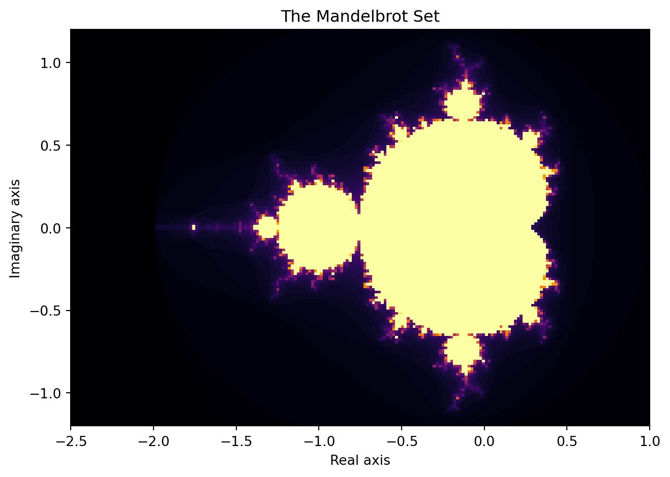
## The Mandelbrot Set {#sec-fractals-mandelbrot}
The **Mandelbrot set** is the most famous fractal,
and the one that persuaded many mathematicians that computation
could be a genuine tool for discovery [@mandelbrot1980].
It lives in the **complex plane**.
For each complex number $c = x + yi$, define the sequence
$$z_0 = 0, \qquad z_{n+1} = z_n^2 + c.$$
The **Mandelbrot set** is the collection of all $c$ for which
this sequence stays bounded.
A key fact makes it computable: if $|z_n| > 2$ for any $n$,
the sequence will escape to infinity.
So we test whether $c$ is in the set by iterating up to some
maximum number of steps and checking whether $|z_n|$ exceeds 2.
We color each point $c$ by how quickly it escapes:
points that escape after 1 step are one color, those that escape
after 10 steps get another, and points that never escape
(within our limit) are drawn black.
The resulting **escape-time map** reveals the Mandelbrot set
and its infinitely intricate fractal boundary.
Here we introduce **NumPy**, a Python library for numerical arrays.
- `import numpy as np` is the standard convention for importing it.
- `np.linspace(a, b, n)` returns an array of `n` evenly spaced values
from `a` to `b`.
- `np.zeros((rows, cols))` creates a two-dimensional array of zeros.
We use `np.linspace` to generate the $x$ and $y$ grid coordinates
and `np.zeros` to store the escape counts.
We then loop over every grid point -- not vectorized, but clear.
The `plt.imshow` function, introduced at @sec-pascal-sierpinski,
turns the 2D count array into a color image.
### Research Example: What Does the Mandelbrot Set Actually Look Like? {.unnumbered .unlisted}
The rule $z \mapsto z^2 + c$ is five characters long. Color every point $c$ in the complex plane by how many steps it takes to escape to infinity. Can one simple rule produce a shape of literally infinite complexity?
```{python}
import numpy as np
import matplotlib.pyplot as plt

def mandelbrot_count(c, max_iter=80):
    z = 0j
    for k in range(max_iter):
        # |z|^2 > 4 equals |z| > 2 but skips a square root
        if z.real * z.real + z.imag * z.imag > 4:
            return k
        z = z * z + c
    return max_iter

width, height = 200, 150
xs = np.linspace(-2.5, 1.0, width)
ys = np.linspace(-1.2, 1.2, height)
counts = np.zeros((height, width))

for row in range(height):
    for col in range(width):
        c = complex(xs[col], ys[row])
        counts[row, col] = mandelbrot_count(c)

fig, ax = plt.subplots(figsize=(8, 5))
ax.imshow(
    counts,
    extent=[-2.5, 1.0, -1.2, 1.2],
    origin='lower',
    cmap='inferno',
    aspect='equal'
)
ax.set_title('The Mandelbrot Set')
ax.set_xlabel('Real axis')
ax.set_ylabel('Imaginary axis')
plt.tight_layout()
plt.show()
```
The black region is the Mandelbrot set itself.
Its boundary is infinitely intricate:
zooming into any edge reveals new spirals, filaments,
and miniature copies of the whole set.
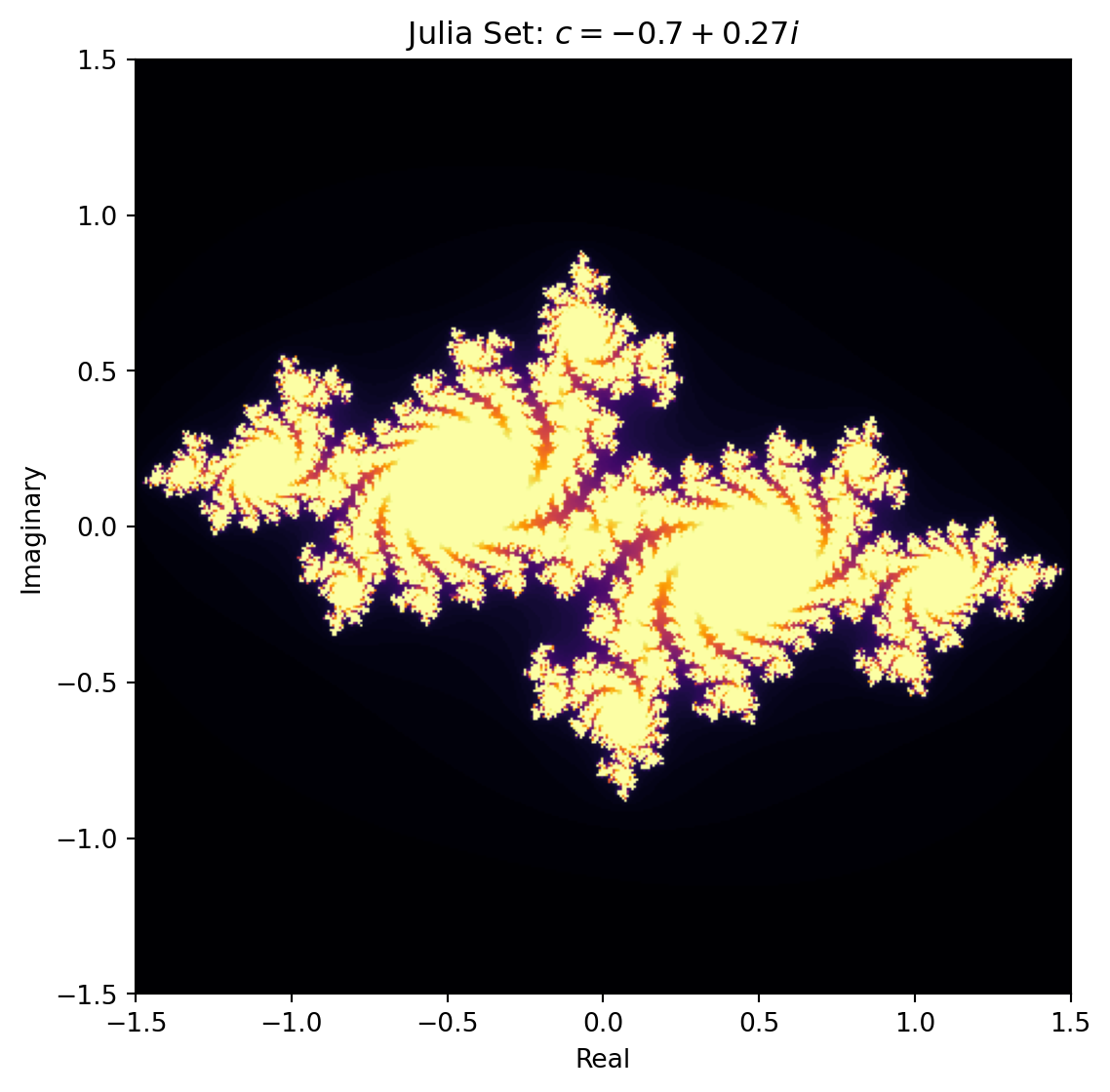
### Research Example: What Does a Julia Set Look Like? {.unnumbered .unlisted}
A related family, the **Julia sets**, comes from fixing $c$
and varying the starting point $z_0$.
For each value of $c$ there is a different Julia set.
Points inside the Mandelbrot set correspond to values of $c$
for which the Julia set is a connected shape;
points outside give $c$ where the Julia set is a Cantor-like dust.
The Mandelbrot set is therefore a **map of Julia sets**:
every point on the boundary corresponds to a dramatic change
in the Julia set's topology.
For $c = -0.7 + 0.27i$ — a value just inside the Mandelbrot boundary —
what does its Julia set actually look like?
```{python}
#| label: fig-fractals-julia
#| fig-cap: "Julia set for c = −0.7 + 0.27i. Each pixel's color encodes how many iterations the starting point z₀ took to escape; black pixels never escaped within 100 steps."
import numpy as np
import matplotlib.pyplot as plt

c_julia = complex(-0.7, 0.27)
width, height = 400, 400
xs_j = np.linspace(-1.5, 1.5, width)
ys_j = np.linspace(-1.5, 1.5, height)
Z = xs_j[np.newaxis, :] + 1j * ys_j[:, np.newaxis]
counts_j = np.full((height, width), 100)
active = np.ones((height, width), dtype=bool)
for k in range(100):
    Z[active] = Z[active]**2 + c_julia
    escaped = active & (Z.real**2 + Z.imag**2 > 4)
    counts_j[escaped] = k
    active[escaped] = False

fig, ax = plt.subplots(figsize=(6, 6))
ax.imshow(counts_j, extent=[-1.5, 1.5, -1.5, 1.5],
          origin='lower', cmap='inferno', aspect='equal')
ax.set_title(r'Julia Set: $c = -0.7 + 0.27i$')
ax.set_xlabel('Real')
ax.set_ylabel('Imaginary')
fig.tight_layout()
plt.show()
```
The Julia set for this value of $c$ is a connected, intricately branched shape — infinitely detailed at every scale. Change $c$ by a tiny amount and the shape transforms completely, which is why the Mandelbrot set serves as its map: every point on the Mandelbrot boundary marks a dramatic change in the corresponding Julia set's structure.
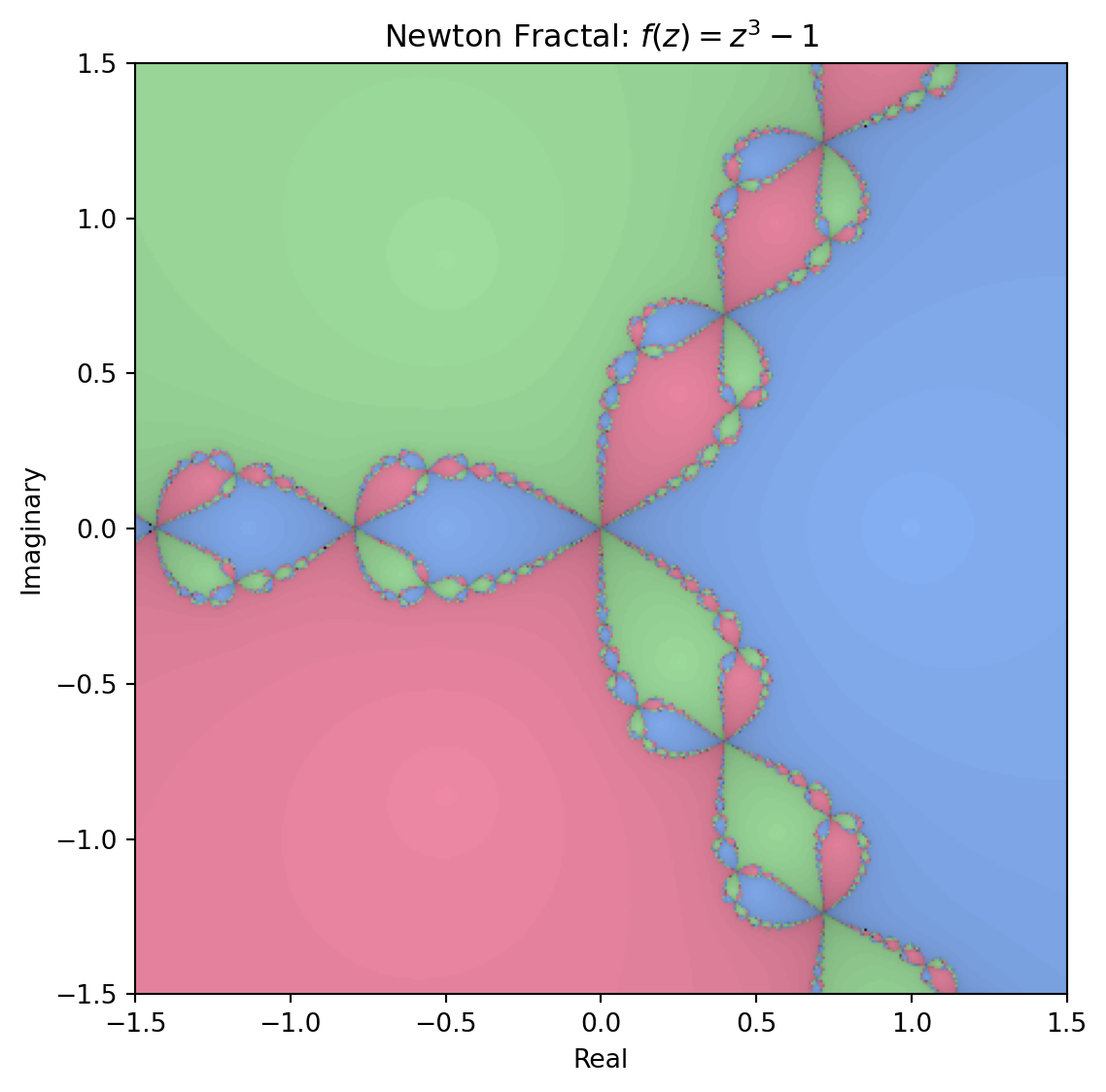
### Research Example: Where Do Newton's Steps Lead? {.unnumbered .unlisted}
Newton's method for finding roots of a polynomial creates a fractal
by a different mechanism.
For $f(z) = z^3 - 1$, three cube roots of unity compete to
attract each starting point.
Color each starting point by which root it converges to — do the three territories have smooth borders, or do all three meet at every boundary point?
```{python}
#| label: fig-fractals-newton
#| fig-cap: "Newton fractal for z³ − 1. Three colors mark which cube root each starting point converges to; brightness encodes convergence speed."
import numpy as np
import matplotlib.pyplot as plt

width, height = 400, 400
xs_n = np.linspace(-1.5, 1.5, width)
ys_n = np.linspace(-1.5, 1.5, height)
Z = xs_n[np.newaxis, :] + 1j * ys_n[:, np.newaxis]
roots_n = [1+0j, np.exp(2j*np.pi/3), np.exp(4j*np.pi/3)]
root_id = np.zeros((height, width), dtype=int)
speed_n = np.zeros((height, width))
active  = np.ones((height, width), dtype=bool)
max_iter = 40
for k in range(max_iter):
    Z2 = Z * Z
    denom = 3 * Z2
    safe = active & (np.abs(denom) > 1e-10)
    Z[safe] -= (Z[safe] * Z2[safe] - 1) / denom[safe]
    for i, r in enumerate(roots_n):
        hit = safe & (np.abs(Z - r) < 1e-6) & (root_id == 0)
        root_id[hit] = i + 1
        speed_n[hit]  = 1.0 - k / max_iter
        active[hit]   = False

palette = np.array([[0.537, 0.706, 0.980],
                    [0.635, 0.890, 0.631],
                    [0.953, 0.545, 0.659]])
img = np.zeros((height, width, 3))
for i in range(3):
    mask = (root_id == i + 1)[..., np.newaxis]
    bright = (0.4 + 0.6 * speed_n)[..., np.newaxis]
    img += mask * palette[i] * bright

fig, ax = plt.subplots(figsize=(6, 6))
ax.imshow(img, extent=[-1.5, 1.5, -1.5, 1.5], origin='lower', aspect='equal')
ax.set_title(r'Newton Fractal: $f(z) = z^3 - 1$')
ax.set_xlabel('Real')
ax.set_ylabel('Imaginary')
fig.tight_layout()
plt.show()
```
The three territories have no clean borders — every boundary point is simultaneously on the edge of all three basins, making the fractal boundary infinitely tangled. A small step in any direction can land you in a completely different basin, which is why Newton's method can behave unpredictably when started near one of these boundaries.
## Box-Counting Dimension {#sec-fractals-dimension}
In @sec-pascal-dimension we introduced the fractal dimension formula
$$d = \frac{\log N}{\log(1/r)},$$
where $N$ is the number of self-similar copies and $r$ is the
scaling ratio.
For self-similar fractals with exact scaling this gives an exact answer.
For the **Koch snowflake**: each step replaces one segment with
$N = 4$ segments, each scaled by $r = 1/3$.
$$d_{\text{Koch}} = \frac{\log 4}{\log 3} \approx 1.2619.$$
For the **Sierpinski triangle**: each step produces $N = 3$ copies
scaled by $r = 1/2$.
$$d_{\text{Sierp}} = \frac{\log 3}{\log 2} \approx 1.5850.$$
Both fall between 1 and 2.
The Koch snowflake is more than a curve but less than a filled region;
the Sierpinski triangle falls between a curve and a plane region [@hausdorff1918].
### Research Example: What Dimension Are These Fractals? {.unnumbered .unlisted}
Ordinary shapes have integer dimensions: a line is 1, a filled square is 2. Fractals live in between. Can we compute the exact dimension of the Koch snowflake and the Sierpinski triangle using nothing more than a logarithm?
```{python}
import math

print("Koch snowflake:")
print("  N=4 copies, scale r=1/3")
d = math.log(4) / math.log(3)
print(f"  dimension = log(4)/log(3) = {d:.4f}")
print()
print("Sierpinski triangle:")
print("  N=3 copies, scale r=1/2")
d = math.log(3) / math.log(2)
print(f"  dimension = log(3)/log(2) = {d:.4f}")
```
Not all fractals have exact self-similarity --
the Mandelbrot boundary is statistically self-similar
but not geometrically exact.
The **box-counting dimension** is a numerical method
that works for any fractal.
Cover the fractal with a grid of boxes of side length
$\varepsilon$, and let $N(\varepsilon)$ be the number of
boxes that contain part of the fractal.
For a fractal of dimension $d$,
$$N(\varepsilon) \approx C \cdot \varepsilon^{-d},$$
so a log-log plot of $N$ against $1/\varepsilon$ has slope $d$.
### Research Example: Can We Measure a Fractal's Dimension Numerically? {.unnumbered .unlisted}
The Mandelbrot boundary has no exact self-similarity ratio, so the simple formula $d = \log N / \log(1/r)$ cannot help. Can we cover the Sierpinski triangle with grids of different sizes, count how many boxes are needed each time, and recover the correct dimension $\log 3 / \log 2 \approx 1.585$ from the slope of a log-log plot?
The code below generates 100,000 chaos-game points for the
Sierpinski triangle and estimates the dimension by linear regression
in log-log space.
Finer grids (larger scale factor $s = 1/\varepsilon$) stay in the
fractal scaling regime; very coarse grids see only the bounding box
and underestimate the dimension.
```{python}
import random
import math

random.seed(0)
verts = [(0.0, 0.0), (1.0, 0.0), (0.5, 3**0.5 / 2)]
x, y = verts[0]
pts = []
for _ in range(100_000):
    vx, vy = random.choice(verts)
    x = (x + vx) / 2
    y = (y + vy) / 2
    pts.append((x, y))

scales = [8, 16, 32, 64, 128]
log_s, log_N = [], []
for s in scales:
    boxes = set()
    for px, py in pts:
        boxes.add((int(px * s), int(py * s)))
    n_boxes = len(boxes)
    log_s.append(math.log(s))
    log_N.append(math.log(n_boxes))
    print(f"scale {s:>3}: {n_boxes:>5} boxes")

n = len(log_s)
mean_x = sum(log_s) / n
mean_y = sum(log_N) / n
slope = (
    sum((xi - mean_x) * (yi - mean_y)
        for xi, yi in zip(log_s, log_N))
    / sum((xi - mean_x)**2 for xi in log_s)
)
print(f"\nEstimated dimension:  {slope:.4f}")
theory = math.log(3) / math.log(2)
print(f"Theoretical log(3)/log(2): {theory:.4f}")
```
Observe that the box counts are very close to the powers of three:
$3^3 = 27$, $3^4 = 81$, $3^5 = 243$, $3^6 = 729$, $3^7 = 2187$.
At scale $s = 2^k$ the Sierpinski structure fills exactly $3^k$ boxes,
because each of the $3^k$ sub-triangles at depth $k$ occupies its
own box.
The slight deviation at the largest scales comes from the finite
number of chaos-game points not quite reaching every last box.
The estimated dimension (near 1.585) agrees with the theoretical
value to three or four decimal places.
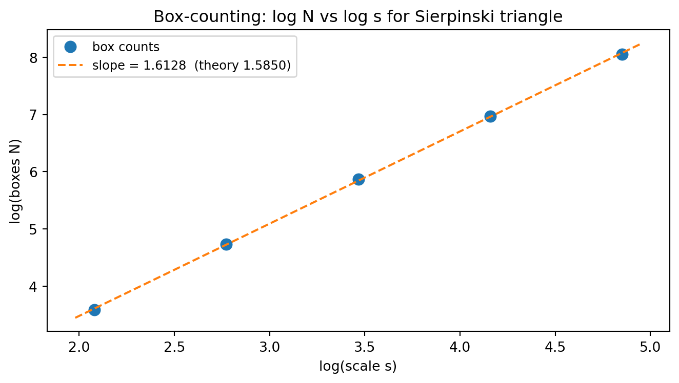
The log-log plot shows this directly: the points fall on a straight line
whose slope is the fractal dimension itself.
```{python}
#| label: fig-fractals-loglog
#| fig-cap: "Box-counting log-log plot for the Sierpinski chaos game. The slope of the fitted line is the estimated fractal dimension ≈ 1.585, matching log(3)/log(2) to four decimal places."
import random, math, matplotlib.pyplot as plt
BLUE   = '#1f77b4'
ORANGE = '#ff7f0e'

random.seed(0)
verts = [(0.0, 0.0), (1.0, 0.0), (0.5, 3**0.5 / 2)]
x, y = verts[0]
pts = []
for _ in range(100_000):
    vx, vy = random.choice(verts)
    x = (x + vx) / 2
    y = (y + vy) / 2
    pts.append((x, y))

scales = [8, 16, 32, 64, 128]
log_s, log_N = [], []
for s in scales:
    boxes = set()
    for px, py in pts:
        boxes.add((int(px * s), int(py * s)))
    log_s.append(math.log(s))
    log_N.append(math.log(len(boxes)))

n = len(log_s)
mean_x = sum(log_s) / n
mean_y = sum(log_N) / n
slope = (sum((xi - mean_x) * (yi - mean_y) for xi, yi in zip(log_s, log_N))
         / sum((xi - mean_x)**2 for xi in log_s))
theory = math.log(3) / math.log(2)
a_int  = mean_y - slope * mean_x
fit_xs = [log_s[0] - 0.1, log_s[-1] + 0.1]
fit_ys = [a_int + slope * x for x in fit_xs]

fig, ax = plt.subplots(figsize=(7, 4))
ax.plot(log_s, log_N, 'o', color=BLUE, ms=8, label='box counts')
ax.plot(fit_xs, fit_ys, '--', color=ORANGE, lw=1.5,
        label=f'slope = {slope:.4f}  (theory {theory:.4f})')
ax.set_xlabel('log(scale s)')
ax.set_ylabel('log(boxes N)')
ax.set_title('Box-counting: log N vs log s for Sierpinski triangle')
ax.legend(fontsize=9)
fig.tight_layout()
plt.show()
```
The points fall almost perfectly on a straight line, and the slope matches $\log 3 / \log 2 \approx 1.585$ to three decimal places. Box-counting turns a visual intuition — "this fractal feels between a line and a filled region" — into a precise, measurable number that you can compute for any shape, even one without exact self-similarity.
## Further Research Topics {#sec-fractals-research}
2. **Koch curve variations.**
The standard Koch curve uses a 60-degree equilateral bump.
Replace the bump with a square (four segments of length $r = 1/4$)
to get the Minkowski sausage, or vary the bump angle away from
60 degrees.
How does the bump angle affect the fractal dimension?
For what angles does the curve self-intersect, and what shape
does it converge to in the self-intersecting regime?
*(Problem proposed by Claude Code.)*
5. **Box-counting dimension of the logistic map attractor.**
In @sec-logistic-bifurcation we saw that above $r \approx 3.57$
the logistic map visits a chaotic attractor, a fractal subset of
$[0, 1]$.
Collect 500,000 orbit values at $r = 3.8$ (discarding the first
1,000 transients) and estimate the box-counting dimension.
Repeat for $r = 3.7$, $r = 3.9$, and $r = 4.0$.
How does the dimension change as $r$ increases toward 4?
Is the dimension of the chaotic attractor at $r = 4$ exactly 1?
*(Problem proposed by Claude Code.)*
6. **The coastline paradox.**
The measured length of a coastline depends on the ruler length:
a short ruler follows every cove, a long ruler skips over them.
This is Richardson's law [@richardson1961]: $L(\varepsilon) \approx C \cdot
\varepsilon^{1-d}$, where $d$ is the fractal dimension.
Find a publicly available coastline boundary in GeoJSON or
shapefile format, apply box-counting to the set of boundary
coordinates, and estimate the fractal dimension.
Compare a smooth coast (Gulf of Mexico) to a rugged one
(Norwegian fjords or the Maine coast).
*(Problem proposed by Claude Code.)*
7. **Dragon curve.**
Fold a strip of paper in half repeatedly in the same direction,
then unfold and stand every fold at a right angle.
The resulting curve is the Heighway dragon [@gardner1967].
It can also be generated by an IFS with two contracting maps.
Plot the dragon curve for 14 levels of folding.
Does it self-intersect?
What is its fractal dimension?
The curve tiles the plane -- can you find the tiling?
*(Problem proposed by Claude Code.)*
8. **L-systems.**
An L-system is a string rewriting rule.
For the Koch curve: start with "F", and replace each "F" with
"F+F$-\!-$F+F" (where "+" turns left $60°$ and "$-$" turns right
$60°$).
Implement a general L-system interpreter in Python that maps
each rule to a turtle-graphics drawing command.
Use it to draw the Koch curve, the Sierpinski triangle (hint:
two different types of forward step), and at least one plant-like
L-system from the literature [@lindenmayer1968; @prusinkiewicz1990].
*(Problem proposed by Claude Code.)*
9. **Weierstrass function: continuous but nowhere smooth.**
The function
$W_N(x) = \sum_{k=0}^{N} a^k \cos(b^k \pi x)$
with $0 < a < 1$ and $b$ a positive odd integer is continuous
everywhere but has no tangent line anywhere when $N \to \infty$
[@weierstrass1872; @borwein2006ema, §3.3].
Compute and plot $W_N(x)$ for $N = 5, 10, 20$ with $a = 0.5$,
$b = 7$, $x \in [0, 2]$.
As $N$ grows, how does the graph change?
Apply box-counting to the graph to estimate its fractal dimension.
Theory predicts $d = 2 + \log a / \log b$;
does your numerical estimate agree?
*(Problem proposed by Claude Code.)*
10. **Fractal dimension of natural images.**
Photographs of clouds, forests, and mountain ranges are said to
have fractal structure.
Load a grayscale image (any standard Python image library works)
and apply box-counting to the set of pixels above a chosen
brightness threshold.
Does the estimated dimension depend on the threshold?
Compare a natural scene to a man-made scene such as a building
facade or a circuit board.
*(Problem proposed by Claude Code.)*
11. **Spiral arms of the Mandelbrot set and Fibonacci.**
Zoom into the main cardioid of the Mandelbrot set.
Around the boundary you see a sequence of bulbs, each with its
own cycle length.
The largest bulb has period 2, the next has period 3, then 5,
then 8 -- the Fibonacci numbers.
Between two bulbs of period $p$ and $q$ sits a bulb of period
$p + q$, a process called Farey addition [@mandelbrot1980].
Write code to identify the period of each bulb (by running the
Mandelbrot iteration from a point inside the bulb) and verify the
Fibonacci pattern around the main cardioid.
*(Problem proposed by Claude Code.)*
12. **Multifractals.**
In a simple fractal like the Sierpinski triangle every
sub-region scales the same way.
A **multifractal** has different scaling behavior in different
regions, described by a spectrum of dimensions $f(\alpha)$.
The invariant measure of the logistic map at $r = 4$
(the histogram of orbit values) is multifractal.
Research the definition of the multifractal spectrum and compute
it numerically: divide $[0, 1]$ into $M$ bins, count the
frequency $p_i$ in each bin, and compute the partition function
$Z(q, \varepsilon) = \sum_i p_i^q \cdot \varepsilon^{\tau(q)}$
for a range of $q$ values.
*(Problem proposed by Claude Code.)*
13. **Three-dimensional fractals.**
The Menger sponge [@menger1926] is the 3D analogue of the Cantor set:
divide a cube into $3^3 = 27$ sub-cubes, remove the center and
the six face-centers (leaving 20), and repeat.
The fractal dimension is $\log 20 / \log 3 \approx 2.727$.
Using a 3D NumPy array of booleans to represent which sub-cubes
survive, generate the Menger sponge at depths 0, 1, 2, and 3
(depth 3 needs a $27^3 = 19{,}683$-cell array).
Plot cross-sections using `plt.imshow`.
How many sub-cubes survive at depth 3?
*(Problem proposed by Claude Code.)*
14. **Hausdorff dimension vs. topological dimension.**
The topological dimension of a curve is 1, of a surface is 2.
The Koch curve has topological dimension 1 but Hausdorff dimension
$\log 4 / \log 3 \approx 1.26$.
Mandelbrot originally defined a fractal as any set whose
Hausdorff dimension strictly exceeds its topological dimension.
Research the definition of Hausdorff dimension [@hausdorff1918] (it involves
coverings by sets of diameter at most $\varepsilon$ as
$\varepsilon \to 0$).
Is the Hausdorff dimension always equal to the box-counting
dimension?
Find an example where they differ.
*(Problem proposed by Claude Code.)*
15. **Zooming into the Mandelbrot boundary.**
The Mandelbrot set contains infinitely many miniature copies of
itself, called "baby Mandelbrot sets."
Write code that zooms into a user-specified rectangle of the
complex plane by rerunning the escape-time computation on a fine
grid within that rectangle.
Locate and zoom into one baby Mandelbrot set (the largest one
sits near $c \approx -1.76$).
How many iterations does it take before the baby copy becomes
recognizable?
What is the period of the central bulb of each baby set?
*(Problem proposed by Claude Code.)*
16. **The Cantor function and the devil's staircase.**
The Cantor set from @sec-fractals-intro is connected to one of the
strangest functions in mathematics: the **Cantor function**,
nicknamed the "devil's staircase" [@cantor1883].
Build it iteratively: at each depth $d$, hold the function constant
at its midpoint value on every removed interval and let it rise
linearly on the surviving Cantor intervals.
At depth 1 the function is constant $\tfrac{1}{2}$ on
$(\tfrac{1}{3}, \tfrac{2}{3})$ and rises linearly on the two
flanking pieces.
At depth 2 it adds flat steps at $\tfrac{1}{4}$ and $\tfrac{3}{4}$
on the next two removed intervals.
Implement this for depths 1 through 6 and plot each stage.
The limiting function is continuous and nondecreasing, yet its
derivative is zero at every point of the Cantor set and it manages
to climb all the way from 0 to 1.
Compute numerically what fraction of the total rise of the
function occurs on intervals removed by depth $d$; show that
this fraction approaches 1 as $d \to \infty$.
Since the Cantor set has total length zero, where does the staircase
"find room" to rise?
Can you construct an analogous staircase for the Cantor set built
by removing middle fifths instead of middle thirds?
*(Problem proposed by Claude Code.)*
17. **The Mandelbrot set as a parameter atlas for the logistic map.**
In @sec-logistic-bifurcation the logistic map
$x_{n+1} = rx_n(1-x_n)$ produced period-doubling bifurcations at
$r \approx 3,\ 3.449,\ 3.544,\ 3.569, \ldots$
The substitution $z = r\!\left(\tfrac{1}{2} - x\right)$ converts
each logistic step into a Mandelbrot step $z_{n+1} = z_n^2 + c$
with $c = \tfrac{r}{2} - \tfrac{r^2}{4}$.
This means the real axis of the Mandelbrot set is literally the
parameter axis of the logistic map, compressed and shifted [@feigenbaum1978; @mandelbrot1980].
Verify numerically: the first bifurcation at $r \approx 3$
should map to $c = -\tfrac{3}{4}$, the exact boundary between
the main cardioid and the period-2 bulb of the Mandelbrot set.
Convert each of the four logistic bifurcation values listed above
to a $c$ value and confirm that each one lands on a known
Mandelbrot period-doubling boundary.
Using Feigenbaum's constant from @sec-logistic-feigenbaum,
predict where the $n$-th bifurcation sits on the real $c$-axis
and check whether the spacing of the Mandelbrot period-doublings
shrinks by the same ratio $\delta \approx 4.669$.
What does this tell you about whether the Feigenbaum constant is
a property of the logistic map specifically, or of a wider class
of one-parameter families?
*(Problem proposed by Claude Code.)*
18. **Lyapunov fractals.**
A **Lyapunov fractal** colors each point $(a, b)$ in the parameter
plane by the Lyapunov exponent of an alternating-parameter logistic
orbit.
Choose a "symbol string" such as "AABAB": each letter tells you
which parameter to use in step $k$ of the iteration
$x_{k+1} = r_k x_k(1 - x_k)$, where $r_k = a$ when the $k$-th
letter is A and $r_k = b$ when it is B.
After discarding 1,000 warm-up steps, compute the Lyapunov exponent
$$\lambda(a,b) = \frac{1}{N}\sum_{k=1}^{N}
\ln\!\bigl|r_k - 2r_k x_k\bigr|.$$
Color the pixel blue if $\lambda < 0$ (stable orbit) and red if
$\lambda > 0$ (chaotic orbit); map intermediate values to a
gradient.
Implement this for a 300×300 grid of $(a,b)$ values in $[2,4]^2$
with the string "AB", then with "AABAB", and then with "ABBBBA" [@markus1990].
Each string produces a strikingly different image — describe the
symmetry you observe and explain it in terms of what the string
encodes about the orbit.
Find a string that produces a clearly fractal boundary and apply
box-counting to the boundary pixels to estimate its fractal
dimension.
*(Problem proposed by Claude Code.)*
19. **The Apollonian gasket and integer curvatures.**
An **Apollonian gasket** is the figure produced by the following
rule: start with three mutually tangent circles; fill the curved
gap between them with the unique circle tangent to all three;
then fill every new gap with its own tangent circle, forever.
**Descartes' Circle Theorem** (1643, rediscovered by Soddy in 1936)
links the four curvatures $k_i = 1/r_i$ of any four mutually
tangent circles [@soddy1936; @lagarias2002apollonian]:
$$(k_1 + k_2 + k_3 + k_4)^2 = 2(k_1^2 + k_2^2 + k_3^2 + k_4^2).$$
Starting from the configuration with curvatures $(-1, 2, 2, 3)$
(the enclosing circle has negative curvature $-1$; the three inner
circles have radii $\tfrac{1}{2}$, $\tfrac{1}{2}$, $\tfrac{1}{3}$),
every subsequent circle also has an integer curvature.
Write code to generate all circles up to depth 5 by recursively
applying Descartes' theorem, storing each new curvature and center,
and plotting the result.
List every integer curvature that appears; which integers from 1
to 50 are missing?
Researchers conjecture that every sufficiently large positive
integer eventually appears — generate the gasket to depth 8 and
test this conjecture empirically up to curvature 200.
The fractal dimension of an Apollonian gasket is approximately
1.3057; estimate it with box-counting on the set of circle centers
and compare to the theoretical value.
*(Problem proposed by Claude Code.)*